Boston University
OpenBU
http://open.bu.edu
Electrical and Computer Engineering BU Open Access Articles
2017-09-01
Hybrid approximate message
passing
This work was made openly accessible by BU Faculty. Please
share
how this access benefits you.
Your story matters.
Version
Citation (published version): Sundeep Rangan, Alyson K Fletcher, Vivek K Goyal, Evan Byrne,
Philip Schniter. 2017. "Hybrid Approximate Message Passing." IEEE
TRANSACTIONS ON SIGNAL PROCESSING, Volume 65, Issue 17, pp.
4577 - 4592 (16).
https://hdl.handle.net/2144/26517
arXiv:1111.2581v4 [cs.IT] 23 Mar 2017
Hybrid Approximate Message Passing
Sundeep Rangan,
Fellow, IEEE, Alyson K. Fletcher,
Member, IEEE, Vivek K Goyal,
Fellow, IEEE,
Evan Byrne,
Student Member, IEEE, and Philip Schniter,
Fellow, IEEE
Abstract—Gaussian and quadratic approximations of message passing algorithms on graphs have attracted considerable re-cent attention due to their computational simplicity, analytic tractability, and wide applicability in optimization and statistical inference problems. This paper presents a systematic framework for incorporating such approximate message passing (AMP) methods in general graphical models. The key concept is a partition of dependencies of a general graphical model into strong and weak edges, with the weak edges representing small, lineariz-able couplings of varilineariz-ables. AMP approximations based on the Central Limit Theorem can be readily applied toaggregates of manyweak edges and integrated with standard message passing updates on the strong edges. The resulting algorithm, which we call hybrid generalized approximate message passing (HyGAMP), can yield significantly simpler implementations of sum-product and max-sum loopy belief propagation. By varying the partition of strong and weak edges, a performance–complexity trade-off can be achieved. Group sparsity and multinomial logistic regression problems are studied as examples of the proposed methodology.
Index Terms—Approximate message passing, belief propaga-tion, sum-product algorithm, max-sum algorithm, group sparsity, multinomial logistic regression.
I. INTRODUCTION
For high-dimensional optimization and inference problems, message-passing algorithms constructed from graphical mod-els have become widely-used in many fields [2]–[4]. The fun-damental principle of graphical models is to decompose high-dimensional problems into sets of smaller low-high-dimensional problems. The decomposition is represented using a bipartite graph, where the problem variables and factors are represented by the graph vertices and the dependencies between them represented by edges. Message passing methods such as loopy belief propagation (BP) use this graphical structure to perform optimization or approximate inference in an iterative manner.
S. Rangan (email: [email protected]) is with the Department of Electrical and Computer Engineering, New York University, Brooklyn, NY, 11201. His work was supported in part by the National Science Foundation under Grant 1116589 and the industrial affiliates of NYU WIRELESS.
A. K. Fletcher (email: [email protected]) is with the Department of Statistics and Electrical Engineering, the University of California, Los An-geles, CA, 90095. Her work was supported in part by the National Science Foundation under Grant 1254204 and the Office of Naval Research under Grant N00014-15-1-2677.
V. K. Goyal (email: [email protected]) is with the Department of Electrical and Computer Engineering at Boston University, Boston, MA, 02215. His work was supported in part by the National Science Foundation under Grant 1422034.
E. Byrne and P. Schniter (email: [email protected] and
[email protected]) are with the Department of Electrical and Computer Engineering, The Ohio State University, Columbus, OH, 43210. Their work was supported in part by the National Science Foundation under Grant CCF-1527162.
Portions of this work were presented at the IEEE International Symposium on Information Theory [1].
In each iteration, optimization or inference is performed “lo-cally” on the sub-problems associated with each factor, and “messages” are passed between the variables and factors to account for the coupling between these sub-problems.
Recently, so-called “approximate message passing” (AMP) [5]–[7] and generalized AMP (GAMP) [8] methods have been developed for the case where the measurement factors depend weakly on a large number of random variables. By linearizing these weak dependencies, one can simplify standard loopy-BP algorithms and rigorously analyze their behavior in the high-dimensional limit [7]. AMP algorithms of this form have been proposed for maximum a posteriori (MAP) and minimum mean-squared error (MMSE) inference in linear models [5], [6], generalized linear models [8], and generalized bilinear models [9]–[11]. These AMP algorithms, however, assume that the underlying random variables are independent. Similarly, they assume that measurements are conditionally independent given these random variables. Thus, one may wonder how to extend these AMP methods to prior (and/or likelihood) models that include dependencies among variables (and/or measurements). By exploiting such dependencies, one can greatly improve the performance of optimization or inference. (We will show an example of this phenomenon in Section VI.) As one solution, we present Hybrid GAMP (HyGAMP) algorithms for what we call graphical model problems with linear mixing. The basic idea is to partition the edges of the graphical model intoweakandstrongsubsets and represent the dependencies among the weak edges using a linear transform. Assuming that the individual components of this linear trans-form areindividually weak, the messages propagating on the weak edges can be simplified using AMP-style approximations and combined with standard loopy-BP messages on the strong edges. The proposed approach is thus a hybrid of AMP and standard loopy-BP techniques.
We detail the HyGAMP methodology using two common variants of loopy BP: thesum-productalgorithm for inference (i.e., computation of the posterior mean) and the max-sum
algorithm for optimization (i.e., computation of the posterior mode). For the sum-product loopy BP algorithm, we argue that the weak-edge messages can be approximated by Gaussian densities whose mean and variance computations are simpli-fied by the Central Limit Theorem (CLT). For max-sum loopy BP, we argue that the weak-edge messages can use quadratic approximations whose parameters are easily computed using least-squares techniques.
The proposed approach can be considered as a generaliza-tion of theturbo AMPmethod proposed in [12] for clustered-sparse signal recovery. The idea behind turbo AMP is to i) partition the overall factor graph into sub-graphs with weak edges and sub-graphs with strong edges, ii) perform
AMP-style message passing within the weak sub-graphs and standard sum-product BP within the strong sub-graphs, and iii) periodically interchange messages between neighboring sub-graphs. Although the turbo-AMP idea has been applied to channel estimation and equalization, wavelet image denoising, video compressive sensing, hyperspectral unmixing, and other problems in, e.g., [13]–[19], a concrete turbo-AMP algorithm that applies to generic factor graphs has never been stated. HyGAMP fills this gap. Furthermore, turbo AMP methods have been proposed exclusively with sum-product message passing. HyGAMP extends the turbo-AMP idea to max-sum message passing. Going further still, the proposed HyGAMP method generalizes turbo-AMP by allowing factor graphs with vector-valued variable nodes (in the strong and/or weak sub-graphs). As such, HyGAMP facilitates the application of AMP techniques to problems such as group-sparse estimation and multinomial logistic regression, which are outside the reach of AMP and turbo AMP.
The use of AMP-style approximations on portions of a factor graph has also been applied with joint parameter es-timation and decoding for CDMA multiuser detection in [20]; in a wireless interference coordination problem in [21], and in the context of compressed sensing [22, Section 7]. The HyGAMP framework presented here unifies and extends all of these examples and thus provides a systematic procedure for incorporating Gaussian approximations of message passing in a modular manner in general graphical models.
A shorter version of this paper was published in [1]. This longer version includes derivations of the proposed algorithms, additional experiments, and many additional explanations, clarifications, and examples throughout. Note that, since the publication of [1], the HyGAMP methodology has been used to solve a variety of problems, including multiuser detection in massive MIMO [23], [24], inference for neuronal connectivity [25], fitting neural mass spatio-temporal models [26], user activity detection in cloud-radio random access [27], and decoding from pooled data [28].
II. GRAPHICALMODELPROBLEMS WITHLINEARMIXING
Let xandzbe real-valued block column vectors
x= [xT1, . . . ,xTn]T, z= [zT1, . . . ,zTm]T, (1) whereTdenotes transposition, and consider a function of these vectors of the form
F(x,z) :=
m X i=1
fi(xα(i),zi), (2) where, for each i, fi(·) is a real-valued function; α(i) is a subset of the indices{1, . . . , n}; andxα(i)is the concatenation of the vectors {xj, j ∈ α(i)}. We will be interested in computations on this function subject to linear constraints of the form zi= n X j=1 Aijxj=Aix, (3) where each Aij is a real-valued matrix andAi is the matrix with block columns {Aij}n
j=1. We will also let A be the
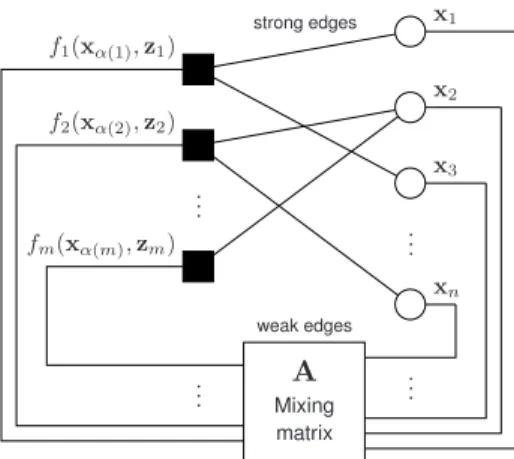
.. . ... .. . .. . x1 x2 x3 xn f1(xα(1),z1) f2(xα(2),z2) fm(xα(m),zm) A Mixing matrix strong edges weak edges
Fig. 1. Factor graph representation of the linear mixing estimation and optimization problems. The variable nodes (circles) are connected to the factor nodes (squares) either directly (strong edges) or via the output of the linear mixing matrixA(weak edges).The basic GAMP algorithm [8] handles the special case where there exists no strong edges and where the variablesxj
are scalar valued.
matrix with block rows {Ai}mi=1, so that we can write the linear constraints simply asz=Ax.
The functionF(x,z)is naturally described via a graphical model as shown in Fig. 1. Specifically, we associate with
F(x,z) a bipartitefactor graph G = (V, E) whose vertices
V consist of n variable nodes corresponding to the (vector-valued) variablesxj andmfactor nodescorresponding to the factorsfi(·) in (2). There is an edge (i, j)∈E in the graph if and only if the variablexj has some influence on the factor
fi(xα(i),zi). This influence can occur in one of two mutually exclusive ways:
• The index j is in α(i), so that the variable xj directly appears in the sub-vectorxα(i)in the factorfi(xα(i),zi). In this case,(i, j)will be called a strong edge, sincexj can have an arbitrary and potentially-large influence on the factor.
• The matrixAijis nonzero, so thatxjaffectsfi(xα(i),zi) through its linear influence onziin (3). In this case,(i, j) will be called aweak edge, since the approximations we will make in the algorithms below assume that Aij are “small.” The set of weak edges into the factor nodeiwill be denotedβ(i).
When we say that Aij are “small,” we mean do not mean small in an absolute sense, but rather thatAij are such that no individual xj can have a significant effect on the sum Pn
j=1Aijxj, and likewise that no individual zi can have a significant effect on the sum Pmi=1zTiAij. One example is when A is drawn with i.i.d. sub-Gaussian entries for sufficiently largemandn. Matrices of this type are assumed in derivation and analysis of the AMP methods [5]–[8].
Together, α(i) and β(i) comprise the set of all indices j
for which a variable node xj is connected to the factor node
fi(·)in the graphG. The union∂(i) =α(i)∪β(i)is thus the neighbor set offi(·). Similarly, for any variable nodexj, we let (with some abuse of notation)α(j)be the set of all indices
edge, and let β(j)be the set of all indicesi for which there exists a weak edge. The union∂(j) =α(j)∪β(j)is thus the neighbor set ofxj.
Given these definitions, we are interested in two problems:
• Optimization problemP-OPT: Given a functionF(x,z)
of the form (2) and a matrixA, compute the maximum: b
x= arg max
x:z=Ax
F(x,z), bz=Axb. (4) Also, for eachj, compute themarginal valuefunction
∆j(xj) := max x\j:z=Ax
F(x,z), (5) wherex\j is composed of{xr}r6=j.
• Expectation problemP-EXP: Given a functionF(x,z)
of the form (2), a matrix A, and scale factor u > 0, define the joint density
p(x) :=Z−1(u) exp [uF(x,z)], z=Ax (6) whereZ(u)is a normalization constant called the parti-tion funcparti-tion (which is a funcparti-tion of u). Then, for this density, compute the expectations
b
x=E[x], bz=E[z]. (7) Also, for eachj, compute the log marginal
∆j(xj) :=
1
ulog
Z
exp [uF(x,z)] dx\j. (8) We include the scale factor u so that the definition of
F(x,z)allows an arbitrary scaling, as in (4).
We now show that P-OPT and P-EXP commonly arise in statistical inference. Suppose that we are given a probability density p(x)of the form (6) for some functionF(x,z). The function F(x,z) may depend implicitly on some observed vector y, so that p(x) represents the posterior density of x given y. In this context, the solution (bx,bz) to the problem
P-OPTis precisely themaximum a posteriori(MAP) estimate
of x and z given the observations y. Similarly, the solution
(xb,bz)to the problemP-EXP is precisely theminimum mean squared error (MMSE) estimate. For P-EXP, the function
∆j(xj)is the log marginal density of xj.
The two problems are related: A standard large deviations argument [29] shows that, under suitable conditions, as u→ ∞ the density p(x) in (6) concentrates around the maxima
(xb,bz)in the solution to the problemP-OPT. As a result, the solution(bx,bz)toP-EXPconverges to the solution toP-OPT. A. Further Assumptions and Notation
In the analysis below, we will assume that, for each factor node fi(·), we have that
α(i)∩β(i) =∅, (9)
i.e., the strong and weak neighbor sets are disjoint. This assumption introduces no loss of generality: If an edge(i, j)is both weak and strong, we can modify the functionfi(xα(i),zi) to “move” the influence ofxj from the termziinto the direct term xα(i). For example, suppose that, for somei,
zi=Ai1x1+Ai3x3+Ai4x4 and α(i) ={1,2}.
In this case, the edge (i,1) is both strong and weak. That is, the function fi(xα(i),zi) depends on x1 through both xα(i) and throughzi. To satisfy assumption (9), we define
znewi =Ai3x3+Ai4x4
finew(xα(i),znewi ) =fi((x1,x2),Ai1x1+znewi ), under which fi(xα(i),zi) =finew(xα(i),znewi ). Thus we can replacefi(·)andzi withfinew(·)andznewi that obey (9).
Even when the dependence of a factor fi(xα(i),zi) on a variable xj is only through the linear term zi, we may still wish to “move” the dependence to a strong edge. The reason is that the HyGAMP algorithm is designed around the assumption that the linear dependence is weak, i.e., that the elements in Aij are small. If these elements are not small, then modeling the dependence with a strong edge improves the accuracy of HyGAMP at the expense of greater computation. One final notation: sinceAij 6=0only when j∈β(i), we may sometimes write the summation (3) as
zi= X j∈β(i)
Aijxj=Ai,β(i)xβ(i), (10) wherexβ(i) is the sub-vector ofxwith componentsj∈β(i)
andAi,β(i)is the corresponding sub-matrix ofAi. III. MOTIVATINGEXAMPLES
We begin with a basic development to show that problems with a fully separable prior and likelihood fit within our model. Then we show an extension to more complicated problems. More detailed examples are deferred to Sections VI and VII. Linear Mixing and General Output Channel—Independent Sub-Vectors: As a simple example of a graphical model with linear mixing, consider the following estimation problem: An unknown vectorxhas independent sub-vectorsxj, each with a joint probability densityp(xj). The vectorxis passed through a linear transform to yield an outputz=Ax. Each sub-vector zi then randomly generates an output yi with conditional density p(yi|zi). The goal is to estimate x given A, the observationsy, and knowledge of the densities.
Common applications of this formulation include the fol-lowing. In compressive sensing [22], x is a sparse vector andA is a sensing matrix. The measurementsy are usually modeled as z plus Gaussian noise, in which case p(yi|zi) is Gaussian. In binary linear classification [30], the rows of A are training feature vectors, the elements of y are binary training labels, and xis a weight vector learned to predict a label from its feature vector. Here, p(yi|zi)is an “activation function” that accounts for error in the linear-prediction model, often based on the logistic sigmoid. When n > m, a sparse weight vectorxis sought to avoid over-fitting [31]. Indigital communicationssettings,xmight be a vector of finite-alphabet symbols and A a matrix representing the cumulative effect of the modulation, propagation channel, and demodulation [20]. Alternatively, x might represent the channel impulse response, in which case A is constructed from a training symbol sequence [13]. In either case, p(yi|zi) is usually chosen as Gaussian, although a heavy-tailed distribution can be chosen to model impulsive noise [17].
.. . .. . .. . ... x1 x2 x3 xn p(x1) p(x2) p(x3) p(xn) p(y1|z1) p(y2|z2) p(ym|zm) y1 y2 ym A output measurements measurement channels mixing matrix input variables componentwise prior
Fig. 2. An example of a simple graphical model for an estimation problem wherexhas independent components with priorsp(xj),z=Ax, and the
observation vectoryis the output of a componentwise measurement channel with transition functionp(yi|zi).
Under the assumption that the components xj are inde-pendent and the componentsyiare conditionally independent givenz, the posterior density onx factors as
p(x|y) = 1 Z(y) m Y i=1 p(yi|zi) n Y j=1 p(xj), z=Ax, whereZ(y) is a normalization constant. For a fixed observa-tion y, we can write this posterior as
p(x|y)∝exp [F(x,z)], z=Ax,
whereF(x,z)is the log posterior, i.e.,
F(x,z) = m X i=1 logp(yi|zi) + n X j=1 logp(xj),
and the dependence on y is implicit. The log posterior is therefore in the form of (2) with scale factoru= 1andm+n
factors{fi(·)}mi=1+n. The firstmfactors can be assigned as
fi(zi) = logp(yi|zi), i= 1, . . . , m, (11) which do not directly depend on the termsxj. Thusα(i) =∅
for each i= 1, . . . , m. The remainingnfactors are then
fm+j(xj) = logp(xj), j= 1, . . . , n. (12) For these factors, the strong edge set is the singletonα(m+
j) ={j}forj = 1, . . . , n, and there is no linear term; we can think of {zm+j}nj=1 as zero-dimensional. The corresponding factor graph with the m+nfactors is shown in Fig. 2.
In the case when all xj and zi are scalars, the estima-tion problem is precisely the one targeted by GAMP [8], as mentioned in the introduction. The special subcase of measurements in additive white Gaussian noise (AWGN), i.e.,
yi=zi+wi, wi∼ N(0, σw2), (13) is the one targeted by AMP [5]–[7].
Linear Mixing and General Output Channel—Dependent Sub-Vectors: We now consider the significantly more general graphical model framework shown in Fig. 3. In this case, the input sub-vectors xj may be statistically dependent on one another, with dependences described by a graphical model. Some additional latent variables, in a vector u, may also be involved. For example, [12] used a discrete Markov chain to model clustered sparsity, [16] used discrete-Markov and
.. . .. . .. . .. . .. . x1 x2 x3 xn u1 u2 uk p(x1|u) p(x2|u) p(x3|u) p(xn|u) p(y1|z1,v) p(y2|z2,v) p(ym|zm,v) y1 y2 ym v1 v2 A output parameters output measurements measurement channels mixing matrix input variables componentwise prior input parameters
Fig. 3. A generalization of the model in Fig. 2, where the input variables xare themselves generated by a graphical model with latent variables u. Similarly, the dependence of the observation vector yon the linear mixing outputzis through a second graphical model.
Gauss-Markov chains to model slow changes in support and amplitude across multiple measurement vectors, and [14] used a discrete Markov tree to model persistence across scale in the wavelet coefficients of an image. In Section VI, we will detail the application of HyGAMP to group sparsity.
Similarly, the likelihood need not be separable in{yi}. For example, the observations yi can depend on the outputs zi through a second graphical model that may include additional latent variablesvi. For example, the distribution of y1 given z1may depend on unknown parametersvthat also affect the distribution ofy2givenz2. This technique was used in [13] to incorporate constraints on LDPC coded bits when performing turbo sparse-channel estimation, equalization, and decoding using GAMP. In Section VII, we will detail the application of HyGAMP to multinomial logistic regression.
IV. REVIEW OFLOOPYBELIEFPROPAGATION
Finding exact solutions to high-dimensional P-OPT and
P-EXP problems is generally intractable because they require
optimization or expectation overnvariablesxj. A widely-used approximation method is loopy BP [3], [32], which reduces the high-dimensional problem to a sequence of low-dimensional problems associated with each factor fi(xα(i),zi). We con-sider two common variants of loopy BP: the max-sum algo-rithm (MSA) for the problem P-OPT and the sum-product algorithm (SPA) for the problem P-EXP. This section will briefly review these methods, as they will be the basis of the HyGAMP algorithms described in Section V.
The MSA iteratively passes estimates of the marginal utili-ties∆j(xj)in (5) along the graph edges. Similarly, the SPA passes estimates of the log marginals∆j(xj)in (8). For either algorithm, we index the iterations byt= 0,1,2, ...and denote the “message” from the factor nodefi to the variable nodexj in thetth iteration by∆i→j(t,xj)and the reverse message by
∆i←j(t,xj).
To describe the message updates, we introduce some addi-tional notation. First, we note that SPA and MSA messages are equivalent up to a constant offset. That is, adding any constant (w.r.t.xj) to either∆i→j(t,xj)or∆i←j(t,xj) has no effect on the algorithm. Thus, we will use “≡” for equality up to a constant offset, i.e.,
for some constantCthat does not depend onx. Similarly, we write p(x) ∝ q(x) when p(x) = Cq(x) for some constant
C. Finally, for the SPA, we will fix the scale factoru >0in the problemP-EXP, and, for any function∆(·), we will write
E[g(x); ∆(·)] to denote the expectation ofg(x)with respect to the densityp(x) associated with∆(·):
E[g(x); ∆(·)] =
Z
g(x)p(x) dx (14)
p(x)∝exp [u∆(x)] (15)
Given these definitions, the updates for the MSA and SPA variants of loopy BP are as follows:
Algorithm 1: Loopy BP: Consider the problemsP-OPT or
P-EXP above for some functionF(x,z)of the form (2) and
matrix A. For the problemP-EXP, fix the scale factor u >
0. The MSA for P-OPT and the SPA forP-EXP iterate the following steps:
0) Initialization: Set t = 0 and, for each (i, j) ∈ E, set
∆i←j(t,xj) = 0.
1) Factor node update:For each edge(i, j)∈E, compute the function Hi→j(t,x∂(i),zi) := fi(xα(i),zi) + X r∈{∂(i)\j} ∆i←r(t,xr). (16) For theMSA, compute:
∆i→j(t,xj)≡ xmax
∂(i)\j
zi=Aix
Hi→j(t,x∂(i),zi), (17) where the maximization is over all variables xr with
r∈∂(i)\j and subject to the constraintzi =Aix. For theSPA, compute:
∆i→j(t,xj)≡
1
ulog
Z
pi→j(t,x∂(i)) dx∂(i)\j, (18) where the integration is over all variablesxr with r∈ ∂(i)\j, andpi→j(t,x∂(i))is the probability density
pi→j(t,x∂(i))∝exp
uHi→j(t,x∂(i),zi=Aix)
.(19) 2) Variable node update:For each(i, j)∈E:
∆i←j(t+1,xj)≡ X ℓ∈{∂(j)\i} ∆ℓ→j(t,xj). (20) Also, let ∆j(t+1,xj)≡ X i∈∂(j) ∆i→j(t,xj). (21) For theMSA, compute:
b
xj(t+1) := arg max xj
∆j(t+1,xj). (22) For theSPA, compute:
b
xj(t+1) :=E[xj; ∆j(t+1,·)]. (23) 3) Increment t and return to Step 1 unless a maximum
number of iterations is exceeded.
When the graphGis acyclic, it can be shown that the MSA and SPA algorithms above converge to the exact solutions
to the P-OPT and P-EXP problems, respectively. When the graph G has cycles, however, the above algorithms are— in general—only approximate, but often quite accurate. The previous two statements assume that the loopy-BP messages are computed exactly, which is feasible when all variables are either Gaussian or discrete, but otherwise difficult—incurring a complexity that is exponential in general. For more details on loopy BP, see [3], [32], [33].
V. HYBRIDGAMP
The HyGAMP algorithm modifies loopy BP by replacing the weak edges with approximations of their cumulative ef-fects. By treating a subset of d dependencies as weak (as in AMP) rather than strong (as in loopy BP), the complexity of handling those dependencies shrinks from exponential in d
to linear in d. In particular, HyGAMP assumes the elements of Aij are small along any weak edge (i, j). Under this assumption, MSA-HyGAMP uses a quadratic approximation of the messages along the weak edges, reducing the factor-node update to a standard least-squares problem. Similarly, SPA-HyGAMP uses a Gaussian approximation of the weak-edge messages and applies the CLT at the factor nodes.
A derivation of the HyGAMP algorithm is given in Ap-pendix A for the SPA and ApAp-pendix B for the MSA. We note that these derivations are “heuristic” in the sense that we do not claim any formal matching between loopy BP and the HyGAMP approximation.
To state the HyGAMP algorithm, we need additional nota-tion. At iterationt, the HyGAMP algorithm produces estimates b
xj(t) and bzi(t) of the vectors xj and zi. Several other intermediate vectors,bpi(t),bsi(t)andbrj(t), are also produced. Associated with each of these vectors are matrices likeQxj(t)
and Qz
i(t) that represent Hessians for the MSA and covari-ances for the SPA. When referring to the inverses of these matrices, we use the notation Q−jx(t) to mean (Qx
j(t))−1. Finally, for any positive definite matrix Q and vector a, we definekak2
Q:=aTQ
−1a, which is a weighted two norm. Algorithm 2: HyGAMP: Consider the problem P-OPT or
P-EXP for some functionF(x,z)of the form (2) and matrix
A. For the problem P-EXP, fix the scale factor u > 0. The
MS-HyGAMP algorithm for P-OPT and the SP-HyGAMP
algorithm forP-EXP iterate the following steps:
0) Initialization:Set t= 0andbsi(−1) = 0∀i, and select some initial values ∆i→j(−1,xj)for each strong edge
(i, j), andbrj(−1) andQrj(−1)for each index j. 1) Variable node update, strong edges: For each strong
edge (i, j), compute ∆i←j(t,xj)≡ X ℓ∈{α(j)\i} ∆ℓ→j(t−1,xj) − 1 2kbrj(t−1)−xjk 2 Qr j(t−1). (24)
2) Variable node update, weak edges: For each variable node j, compute
and Hx j(t,xj,brj,Qrj) = X i∈α(j) ∆i→j(t−1,xj)− 1 2kbrj−xjk 2 Qr j. (26) ForMS-HyGAMP, b xj(t) = arg max xj ∆j(t,xj) (27a) Q−jx(t) = − ∂ 2 ∂x2∆j(t,xj). (27b) ForSP-HyGAMP, b xj(t) = E(xj; ∆j(t,·)) (28a) Qxj(t) = uCov (xj; ∆j(t,·)). (28b) 3) Factor node update, linear step:For each factor nodei,
compute b zi(t) = X j∈β(i) Aijxbj(t) (29a) b pi(t) = bzi(t)−Qpi(t)bsi(t−1) (29b) Qpi(t) = X j∈β(i) AijQxj(t)A T ij. (29c)
4) Factor node update, strong edges:For each strong edge
(i, j), compute: Hiz→j(t,xα(i),zi,pbi,Qpi) :=fi(xα(i),zi) + X r∈{α(i)\j} ∆i←r(t,xr)−1 2kzi−pbik 2 Qpi.(30)
Then, forMS-HyGAMP, compute:
∆i→j(t,xj)
= max
xα(i)\j,zi
Hiz→j(t,xα(i),zi,bpi(t),Qpi(t)), (31) where the maximization is jointly overzi and all com-ponentsxr withr∈ {α(i)\j}.
ForSP-HyGAMP, compute:
∆i→j(t,xj)≡ 1 ulog Z pi→j(t,xα(i),zi) dxα(i)\jdzi, (32) where the integral is overziand all componentsxrwith
r∈ {α(i)\j}, andpi→j(t,xj)is the probability density
pi→j(t,xα(i),zi)∝
exp uHiz→j(t,xα(i).zi,bpi(t),Qpi(t))
. (33) 5) Factor node update, weak edges:For each factor node
i, compute Hz i(t,xα(i),zi,pbi,Qpi) :=fi(xα(i),zi) + X r∈α(i) ∆i←r(t,xr)− 1 2kzi−pbik 2 Qpi. (34a)
Then, forMS-HyGAMP, compute:
(bx0α(i)(t),bz0i(t)) := arg max x,zi Hz i(t,xα(i),zi,pbi(t),Qpi(t)), (34b) Dzi(t) :=−∂ 2 ∂z2 i Hz i(t,bx 0 α(i),bz 0 i,bpi(t),Qpi(t)), (34c)
where the maximization in (34b) is over the sub-vector xα(i) and output vectorzi.
ForSP-HyGAMP, let b
zi0(t) =E(zi), Di−z(t) =uCov(zi), (35) where zi is the component of the pair (xα(i),zi) with the joint density
pi(t,xα(i),zi)∝
exp uHz
i(t,xα(i),zi,pbi(t),Qpi(t))
. (36) Then, for either MS-HyGAMP or SP-HyGAMP com-pute bsi(t) = Q−i p(t) b z0i(t)−bpi(t), (37a) Qis(t) = Qi−p(t)−Q−ip(t)D−iz(t)Q−ip(t).(37b) 6) Variable node update, linear step: For each variable
node j compute Q−jr(t) = X i∈β(j) ATijQsi(t)Aij, (38a) brj(t) = bx(t) +Qrj(t) X i∈β(j) ATijbsi(t). (38b) Increment t and return to Step 1 unless either a maxi-mum number of iterations is exceeded orkbxj(t)−bxj(t−
1)kis sufficiently small.
Although the HyGAMP algorithm above appears much more complicated than standard loopy BP (Algorithm 1), HyGAMP can require dramatically less computation. Recall that the main computational difficulty of loopy BP is Step 1, the factor update. The updates (17) and (18) involve an optimization or expectation over|∂(i)|sub-vectors, where∂(i)
is the set of all sub-vectors connected to the factor nodei. In the HyGAMP algorithm, these computations are replaced by (31) and (32), where the optimization and expectation need only be computed over the strong edge sub-vectorsα(i). If the number of weak edges is large, the computational savings can be dramatic. The other steps of the HyGAMP algorithms are all linear, simple least-square operations, or componentwise nonlinear functions on the individual sub-vectors.
For ease of illustration, we have only presented one form of the HyGAMP procedure. Several variants are possible:
• Discrete distributions: The above description assumed continuous-valued random variables xj. The procedures can be easily modified for discrete-valued variables by appropriately replacing integrals with summations.
• Message scheduling: The above description also only considered a completely parallel implementation where each iteration performs exactly one update on all edges. Other so-called message schedules are also possible and may offer more efficient implementations or better con-vergence depending on the application (e.g., [34]–[36]). VI. APPLICATION TOGROUP-SPARSESIGNALRECOVERY
To illustrate the HyGAMP method, we first consider the group-sparse estimation problem [37], [38]. Although this problem does not utilize the full generality of HyGAMP, it provides a simple example of the HyGAMP method and has a number of existing algorithms that can be compared against.
A. HyGAMP Algorithm
A general version of the group-sparsity problem that falls within the HyGAMP framework can be described as follows. Let x be an n-dimensional vector with scalar components
{xj}nj=1. Vector-valued components could also be considered, but we restrict our attention to scalar components for simplic-ity. The component indicesj of the vectorxare divided into
K (possibly overlapping) groups,G1, . . . , GK ⊆ {1, . . . , n}. We let γ(j)be the set of group indices k such thatj ∈Gk. That is, γ(j)is the set of groups to which the componentxj belongs.
Suppose that each groupGk can be “active” or “inactive”, and each component xj can be non-zero only when at least one group Gk is active for some k ∈ γ(j). Qualitatively, a vector x is sparse with respect to this group structure if it is consistent with only a small number of groups being active. That is, most of the components of x are zero with the non-zero components having support contained in a union of a small number of groups. The group-sparse estimation problem is to estimate the vector x from some measurements y. The traditional (non-group) sparse estimation problem corresponds to the special case when there are n groups of singletons,
Gj ={j}.
There are many ways to model the group-sparse structure in a Bayesian manner, particularly with overlapping groups. For sake of illustration, we consider the following simple model. For each groupGk, letξk∈ {0,1}be a Boolean variable with
ξk = 1 when the groupGk is active and ξk = 0when it is inactive. We call ξk the “activity indicators” and model them as i.i.d. with
P(ξk = 1) = 1−P(ξk= 0) =ρ (39)
for some sparsity rate ρ ∈ (0,1). We assume that, given the vector ξ, the components of x are independent with the conditional densities
xj|ξ∼
0 ifξk= 0 for allk∈γ(j)
V otherwise, (40)
where V is a random variable having the distribution of the componentxj in the event that it belongs to an active group. Finally, suppose that measurement vector y is generated by first passing x through a linear transform z = Ax and then a separable componentwise measurement channel with likelihoodsp(yi|zi). Many other dependencies on the activities of x and measurement models y are possible – we use this simple model for illustration.
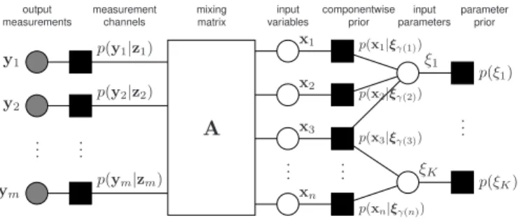
Under this model, the priorxand the measurementsy are naturally described by a graphical model with linear mixing. Due to the independence assumptions, the posterior density of x givenyfactors as p(x|y) = 1 Z(y) m Y i=1 p(yi|zi) n Y j=1 P(xj|ξγ(j)) K Y k=1 P(ξk), (41) where P(xj|ξγ(j))is the conditional density for the random variable in (40). The factor graph corresponding to this distri-bution is shown in Fig. 4.
.. . .. . .. . .. . ... x1 x2 x3 xn ξ1 ξK p(x1|ξγ(1)) p(x2|ξγ(2)) p(x3|ξγ(3)) p(xn|ξγ(n)) p(ξ1) p(ξK) p(y1|z1) p(y2|z2) p(ym|zm) y1 y2 ym A output measurements measurement channels mixing matrix input variables componentwise prior input parameters parameter prior
Fig. 4. Graphical model for the group sparsity problem with overlapping groups. The group dependencies between components of the vector xare modeled via a set of binary latent variablesξ.
Under this graphical model, Appendix C shows that SP-HyGAMP from Algorithm 2 reduces to the simple procedure outlined in Algorithm 3. A similar MS-HyGAMP variant could also be derived. In lines 8 and 9 of Algorithm 3, we used
E(X|R;Qr,ρb)andvar(X|R;Qr,ρb)to denote the expectation and variance, respectively, of the scalar random variable X
with density
X ∼
0 with probability1−bρ
V with probabilityρb; (42)
andRis an AWGN corrupted version of X,
R=X+W, W ∼ N(0, Qr). (43)
Algorithm 3 SP-HyGAMP for group sparsity
1: {Initialization} 2: t←0 3: Qrj(t−1)← ∞ 4: LLRj←k(t−1)←log(ρ/(1−ρ)) 5: ρbj(t)←1−Qk∈γ(j)1/(1 + expLLRj←k(t−1)) 6: repeat
7: {Basic GAMP update}
8: xbj(t)←E(X|R=rbj(t−1);Qrj(t−1),ρbj(t)) 9: Qxj(t)←var(X|R=brj(t−1);Qrj(t−1),bρj(t)) 10: zbi(t)←PjAijbxj(t) 11: Qpi(t)←Pj|Aij|2Qxj(t) 12: pbi(t)←zbi(t)−Qpi(t)bsi(t−1) 13: zbi0(t)←E(zi|pbi(t), Qpi(t)) 14: Qzi(t)←var(zi|pbi(t), Qpi(t)) 15: bsi(t)←(zbi0−pbi(t))/Qpi(t) 16: Qsi(t)←Q−ip(t)(1−Qzi(t)/Qpi(t)) 17: Q−jr(t)←Pi|Aij|2Qsi(t) 18: brj(t)←bxj(t) +Qrj(t) P iAijbsi(t) 19: {Sparsity-rate update} 20: ρbj→k(t)←1−Qi∈{γ(j)\k}1/(1 + expLLRi←k(t−1)) 21: ComputeLLRj→k(t)from (44) 22: LLRj←k(t)←log(ρ/(1−ρ)) +Pi∈{Gk\j}LLRi→k(t) 23: ρbj(t+1)←1−Qk∈γ(j)1/(1 + expLLRj←k(t)) 24: t←t+1 25: untilTerminate
Algorithm 3 can be interpreted as the GAMP procedure from [8] with an additional update of the sparsity rates. Specifically, each iterationt of the algorithm has two stages. The first stage, labeled as the “basic GAMP update,” contains the updates from the basic GAMP algorithm [8], which treats the components xj as independent with sparsity rate ρbj(t). The second stage of Algorithm 3, labeled as the “sparsity-rate update,” updates the sparsity ratesρbj(t)based on the estimates returned by the first stage.
The second stage of Algorithm 3 has a simple interpre-tation. The quantities ρbj(t) and ρbj→k(t) can be interpreted, respectively, as estimates for the probabilities
ρj = Pr ξk= 1 for somek∈γ(j) y ρj→k = Pr ξi= 1for some i∈ {γ(j)\k} y.
That is, ρbj(t) is an estimate of the probability that the componentxjbelongs to at least one active group andρbj→k(t) is an estimate of the probability that it belongs to an active group other than Gk. Similarly, the quantitiesLLRj→k(t)and
LLRj←k(t)are estimates for the log likelihood ratios
LLRk= log P ξk = 1 y P ξk = 0 y.
Most of the updates in the second stage are natural conversions from LLR values to estimates ofρj andρj→k. In line 21, the
LLR message is computed as LLRj→k(t) = log pR(brj(t);Qrj(t),ρb= 1) pR(brj(t);Qrj(t),ρb=ρbj→k(t)) ! , (44) where pR(r;Qr,ρb) is the probability density for the scalar random variableRin (43), whereX has the density (42). The message (44) is the ratio of two likelihoods: the likelihood thatxj belongs to an active group and the likelihood that xj belongs to an active group other than Gk.
To summarize, Algorithm 3 provides a simple and intuitive way to extend the basic GAMP algorithm of [8] to group-structured sparsity.
The HyGAMP algorithm for group sparsity is also ex-tremely general. The algorithm can apply to arbitrary priors and output channels. In particular, the algorithm can incor-porate logistic outputs that are often used for group sparse classification problems [39]–[41]; details are provided in [42]. Also, the method can handle arbitrary, even overlapping, groups. In contrast, the extensions of other iterative algorithms to the case of overlapping groups sometimes requires approx-imations; see, for example, [43]. In fact, the methodology is quite general and likely may be applied to general structured sparsity, including possibly the graphical-model-based sparse structures in image processing considered in [44].
B. Computational Complexity
In addition to its generality, the HyGAMP procedure is among the most computationally efficient for group sparsity. To illustrate this point, consider the special case when there are
Knon-overlapping groups ofdelements each. In this case, the total vector dimension forxisn=Kd. We consider the non-overlapping case since there are many algorithms that apply
Method Complexity
Group-OMP [46] O(ρmn2
)
Group-Lasso [37], [38], [47] O(mn)per iteration
Relaxed BP with vector components [45] O(mn2
)per iteration
HyGAMP with vector components O(mnd)per iteration
HyGAMP with scalar components O(mn)per iteration
TABLE I
COMPLEXITY COMPARISON FOR DIFFERENT ALGORITHMS FOR GROUP SPARSITY ESTIMATION OF A SPARSE VECTOR WITHKGROUPS,EACH GROUP OF DIMENSIONd. THE NUMBER OF MEASUREMENTS ISmAND
THE SPARSITY RATE ISρ.
to this case that we can compare against. For non-overlapping uniform groups, Table I compares the computational cost of the HyGAMP algorithm to other methods.
The computational cost of each iteration of the HyGAMP algorithm, Algorithm 3, is dominated by the matrix mul-tiplications by A (line 10) and AT (line 18) and by the componentwise squares ofAandAT (lines 11 and 17). Each of these operations has O(mn) = O(mdK) cost. Note that the multiplications by componentwise-square matrices can be eliminated by using the scalar-variance version of GAMP [8]. Also, the multiplications by A and AT are relatively cheap if the matrix has a fast transform (e.g., FFT). The other per-iteration computations are themscalar estimates at the output (lines 13 and 14); thenscalar estimates at the input (lines 8 and 9); and the updates of the LLRs. All of these computations are relatively simple.
For the case of non-overlapping groups, the HyGAMP algorithm could also be implemented using vector-valued components. Specifically, the vector x can be regarded as a block vector with K vector components, each of dimension
d. The general HyGAMP algorithm, Algorithm 2, can be applied on the vector-valued components. To contrast this with Algorithm 3, we will call Algorithm 3 HyGAMP with scalar components, and call the vector-valued case HyGAMP with vector components.
The cost is slightly higher for HyGAMP with vector com-ponents. In this case, there are no non-trivial strong edges since the block components are independent. However, in the update (29c), each Aij is 1 ×d and Qxj(t) is d×d. Thus, the computation (29c) requires mK computations of
d2 cost each for a total cost of O(mKd2) = O(mnd), which is the dominant cost. Of course, there may be a benefit in performance for HyGAMP with vector components, since it maintains the complete correlation matrix of all the components in each group. We do not investigate this possible performance benefit in this paper.
Also shown in Table I is the cost of the relaxed BP method from [45], which also uses approximate message passing similar to HyGAMP with vector components. That method, however, performs the same computations as HyGAMP on each of the mK graph edges as opposed to the m +K
graph vertices. It can be verified that the resulting cost has anO(mK2d2) =O(mn2)term.
These message passing algorithms can be compared against widely-used group LASSO methods [37], [38], which estimate x by solving some variant of a regularized least-squares
50 100 150 200 -35 -30 -25 -20 -15 -10 -5 0 5 LMMSE Grp LASSO GAMP Grp OMP Hybrid-GAMP N o rm a liz e d M S E (d B ) Number of Measurementsm
Fig. 5. Comparison of performances of various estimation algorithms for group sparsity withn = 100 groups of dimension d= 4with a sparsity fraction ofρ= 0.1.
problem of the form b x:= arg min x 1 2ky−Axk 2+γ n X j=1 kxjk2, (45) for some regularization parameterγ >0. The problem (45) is convex and can be solved via a number of methods including [47]–[49], the fastest of which is the SpaRSA algorithm of [47]. Interestingly, this algorithm is similar to the GAMP method in that the algorithm is an iterative procedure, where in each iteration there is a linear update followed by a componentwise scalar minimization. Like the GAMP method, the bulk of the cost is theO(mn)operations per iteration for the linear transform. An alternative approach for group sparse estimation is group orthogonal matching pursuit (Group-OMP) of [41], [46], a greedy algorithm that detects one group at a time. Each round of detection requires K correlations of cost md2. If there are on average ρK nonzero groups, the total complexity will be O(ρK2md2) =O(ρmn2). From the complexity estimates summarized in Table I it can be seen that GAMP, despite its generality, is computationally as simple (per iteration) as some of the most efficient algorithms specifically designed for the group sparsity problem.
Of course, a complete comparison requires that we consider the number of iterations, not just the computation per iteration. This comparison requires further study beyond the scope of this paper. However, it is possible that the HyGAMP procedure will be favorable in this regard. Our simulations below show good convergence after only 10–20 iterations. Moreover, in the case of independent (i.e. non-group) sparsity, the number of iterations for AMP algorithms is typically small and often much less than other iterative methods. Examples in [22] show excellent convergence in 10 to 20 iterations, which is dramatically faster than the iterative soft-thresholding method of [50].
C. Numerical Experiments
Fig. 5 shows a simple simulation comparison of the mean squared error (MSE) of the HyGAMP method (Algorithm 3)
along with group OMP, group LASSO, basic GAMP, and the simple linear MMSE estimator. The simulation used a vector x with n = 100 groups of size d = 4 and sparsity fraction of ρ = 0.1. The matrix was i.i.d. Gaussian and the observations were with AWGN noise at an SNR of 20 dB. The number of measurementsmwas varied from 50 to 200, and the plot shows the MSE for each of the methods. The HyGAMP method was run with 20 iterations. In group LASSO, at each value of m, the algorithm was simulated with several values of the regularization parameter γ in (45) and the plot shows the minimum MSE. In Group-OMP, the algorithm was run with the true value of the number of nonzero coefficients. It can be seen that the HyGAMP method is consistently as good or better than both other methods. Furthermore, HyGAMP is significantly better than basic GAMP, which exploits sparsity but not group sparsity. All code for the simulations can be found in the GAMPmatlab package [51].
We conclude that, for the problem of group-sparse recovery from AWGN-corrupted measurements, the HyGAMP method is at least comparable in performance and computational complexity to the most competitive algorithms. On top of this, HyGAMP offers a much more general framework that can include more rich modeling in both the output and input.
VII. APPLICATION TOMULTINOMIALLOGISTIC
REGRESSION
In a second example of the HyGAMP method, we apply it to the problem ofmulticlass linear classificationusing the approach known asmultinomial logistic regression.
A. Multinomial Logistic Regression
Inmulticlass classification[30], one observes a training set
{(ai, yi)}im=1consisting ofmpairs of a feature vectorai∈Rn and a d-ary class label yi ∈ {1, ..., d}. The goal is then to infer the unknownd-ary class labely0 of an observed feature vector a0. In thelinear approach to this problem, we design a weight matrixXb ∈Rn×d from the training set. Then, given an unlabeled feature vector a0, we first generate a vector of linear “scores”z0:=XbTa0∈Rd, and estimate the class label
y0 as the index of the largest score, i.e., b
y0= arg max k
[z0]k. (46)
Multinomial linear regression (MLR) [30] is one of the best known methods to design the weight matrix X. There, the labels {yi} are modeled as conditionally independent given the scores{zi}, wherezi:=XTai. That is,
Pr(y|X;A) =
m Y i=1
pmlr(yi|XTai), (47a) wherepmlr(yi|zi)is the multinomial logistic pmf,
pmlr(yi|zi) := exp [zi]yi Pd k=1exp [zi]k , yi ∈ {1, ..., d}. (47b) The rowsxTj of the weight matrixXare then modeled as i.i.d.,
p(X) =
n Y j=1
For log-convex p(xj), MAP estimation of X is a convex problem. The log-convex Laplacian prior
plap(xj) = (λ/2)dexp −λkxjk1 (49) is a popular choice for p(xj) that promotes sparsity in the designed weight matrix Xb. Sparsity is essential in the case that the feature dimension n is much larger than the number of training examplesm. Fast implementations of sparse MLR were proposed in [31] and refined in [52].
B. HyGAMP Algorithm
Max-sum HyGAMP (MS-HyGAMP) can be directly ap-plied to solve the above optimization problem. To do this, we set Aij = [ai]jId ∀i, j and, recalling (11), we choose
fi(zi) = logpmlr(yi|zi)∀i= 1, ..., m, and recalling (12), we choose fm+j(xj) = logplap(xj) ∀j = 1, ..., n. Then (27a) boils down to b xj= arg min x 1 2(x−brj) T[Qr j] −1(x− brj) +λkxk1, (50) and (34b) boils down to
b zi= arg min z 1 2(z−bpi) T[Qp i] −1(z− b pi)−logpmlr(yi|z). (51) Both problems are convex and can be solved using standard methods, e.g., majorization–minimization or Newton’s method in the case of (51). For more details, including the implemen-tation of (27b) and (34c), we refer the reader to [53].
SP-HyGAMP can also be applied to MLR, again using the likelihood (47). However, rather than the Laplacian prior (49), we suggest choosing the Bernoulli-multivariate-Gaussian prior
p(X) = n Y j=1 pbg(xj) (52a) pbg(xj) =βδ(xj) + (1−β)N(xj;0, qI) (52b) withβ ∈[0,1), which promotes approximate row-sparsity in
b
Xunder sum-product inference. In this case, it can be shown [53] that (28) can be computed in closed form as
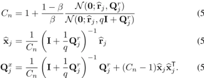
Cn = 1 + 1−β β N(0;brj,Qr j) N(0;brj, qI+Qrj) (53) b xj = 1 Cn I+1 qQ r j −1 brj (54) Qxj = 1 Cn I+1 qQ r j −1 Qrj+ (Cn−1)bxjxbTj. (55) Although we are not aware of a closed-form solution to (35), it can be approximated using numerical integration.
C. Numerical Experiments
We will now describe the results of two experiments used to evaluate the application of HyGAMP to sparse MLR. In these experiments, SP-HyGAMP and MS-HyGAMP were compared to two state-of-the-art sparse MLR algorithms: SBMLR from [54] and GLMNET from [52].
1) Synthetic Data: We first performed an experiment on synthetic data with d = 3 classes, n = 500 features, and
m = 102 examples. The use of synthetic data allowed us to analytically compute the expected test-error rate associated with the designed weight matricesXb.
To generate the synthetic data, we first constructed the set of training labels {yi} such that m/d training samples were dedicated to each class. Then we drew feature vectors {ai} i.i.d. from the class-conditional densityai|yi ∼ N(µyi, vIn).
The class means {µy}dy=1 were10-sparse, with support cho-sen uniformly at random and with non-zero entries chocho-sen uniformly from the columns of a10×10random orthonormal matrix. The parameterv was then chosen to achieve a Bayes error rate of 10%. Thus, only 10 of the 500 features were discriminatory. Note that the data-generation model is not matched to the statistical model assumed in the derivation of MS-HyGAMP or SP-HyGAMP.
To test the algorithms, we performed 12 trials, where in each trial we invoked each algorithm-under-test on randomly generated training data and then computed the resulting ex-pected test-error rate. The SP-HyGAMP algorithm used (52) with parameters (β, q) tuned over a 3×5 logarithmically-spaced grid using 5-fold cross-validation (CV). The GLMNET algorithm, which solves the same convex optimization problem as MS-HyGAMP, tuned λ in (49) over 25 logarithmically-spaced values using5-fold CV. The same CV-optimalλ was then used for MS-HyGAMP. Finally, SBMLR is parameter-free, and thus did not require tuning.
For a designed weight matrixXb = [bx1, ...,xbd], the expected test-error rate can be analytically computed [53] as
Pr{err}= 1−1 d d X y=1 Pr{cor|y} (56) Pr{cor|y}= Pr\ k6=y n (bxy−bxk)Ta<(xby−xbk)Tµy o , (57) wherea∼ N(0, vIn)and the multivariate normal cdf in (57) was computed using Matlab’smvncdf.
In addition to computing the expected test-error rate, we computed two metrics for the sparsity of the designed weight matrices. The metricKbℓ0 =kXbk0quantifies absolute sparsity,
i.e., the number of non-zero elements in Xb. But since the weights returned by SP-HyGAMP are non-zero with probabil-ity one, we also computed the “effective sparsprobabil-ity”Kb99, which is defined as the minimum number of elements inXb required to reach99%ofkXbk2
F.
Table II shows the expected test-error rate,Kb99, andKbℓ0 of
each algorithm, averaged over 12 independent trials. From this table, we see that MS-HyGAMP and GLMNET matched on all metrics. This result is expected because the two algorithms aim to solve the same convex problem, and it offers evidence that they do in fact solve the problem. Thus, in the sequel, we report only the results of GLMNET. Next, Table II shows that the SP-HyGAMP achieved the best expected test-error rate of13.981%, with SBMLR achieving the second best. For comparison, we recall that the Bayes (i.e., minimum) expected error rate was 10%in this experiment. The table also shows
Algorithm % Error Kb99 Kbℓ0 GLMNET 14.787 13.25 25.75 MS-HyGAMP 14.787 13.25 25.75 SBMLR 14.059 15.08 28.92 SP-HyGAMP 13.981 16.08 1500 TABLE II
RESULTS FOR THE SYNTHETIC DATA EXPERIMENT
that the (average) effective sparsity Kb99 was similar for all algorithms, and smaller than the sparsity of the Bayes’ optimal classifier for this dataset, which is Kbℓ0= 30.
2) Handwritten Digit Classification: In the second ex-periment, we tested SP-HyGAMP, GLMNET, and SBMLR on the Mixed National Institute of Standards and Technol-ogy (MNIST) dataset [55]. The MNIST dataset consists of
m = 70 000 total images of handwritten digits 0 through
9, hence d = 10. Each image has n = 784 pixels. In this experiment we performed 24 trials, where in each trial we randomly partitioned the total dataset into a training and testing portion. Within each trial, we varied the number of image samples in the training partition from m = 56 to
m= 1000. Using the training data, we used each algorithm-under-test to design a weight matrix, which was then used to compute an empirical error-rate on the test partition of the dataset. In this experiment, SP-HyGAMP and GLMNET tuned their associated parameters in a similar manner as in the synthetic experiment. However, they used 2-fold CV instead of5-fold CV to reduce computation.
Figure 6 shows the empirical test-error rate versus the number of training samples m, averaged over the24random trials. The error bars indicate the standard deviation of the empirical error-rate estimate. The figure shows that, for allm, SP-HyGAMP achieved the best test-error rate and GLMNET achieved the second best. The figure also shows that, for all algorithms, the test-error rate decreased to a common value as the number of training samples m increased. This is not surprising; we expect that, with enough training data, any reasonable approach should recover a close approximation to the Bayes-optimal linear classifier. A much more difficult problem is designing a good linear classifier from limited training data, and, for this problem, Figure 6 shows that SP-HyGAMP beats the competition.
D. Simplified HyGAMP and EM/SURE Tuning
When directly applied to multinomial logistic regression, each iteration of HyGAMP involves the update ofO(m+n)
multivariate Gaussian pdfs, each of dimension d, for a total complexity of O((m+n)d3) per iteration. This complexity can be quite large in practice, especially relative to state-of-the-art methods like GLMNET and SBMLR. Furthermore, in its more direct form, HyGAMP assumes knowledge of the statistical parameters of its prior and likelihood. In order to tune these parameters to the data, it was suggested above to use cross-validation (as with GLMNET). But K-fold cross-validation of P parameters using G hypothesized values of each parameter requires the training and evaluation of KGP classifiers, which can be very expensive in practice.
102 103 0 0.1 0.2 0.3 0.4 0.5 0.6 SP-HyGAMPSBMLR GLMNET T e s t-E rr o r R a te
Number of Training Samplesm
Fig. 6. Classification results for MNIST dataset.
Fortunately, for multinomial logistic regression, it is possi-ble to modify HyGAMP in such a way that the complexity of the resulting method becomes competitive with GLMNET and SBMLR. The modification consists of two parts: i) a simplification of HyGAMP wherein the covariance matrices Qrj,Qxj,Qpi,Qzi are constrained to be diagonal; and ii) an application of EM-based [56] and SURE-based [57] parameter tuning to the priors and likelihoods relevant to multinomial lo-gistic regression. A complete description of EM/SURE-tuned simplified HyGAMP (SHyGAMP) for multinomial logistic regression can be found in [58], with full derivations in [53]. In [58], a detailed numerical study establishes that EM/SURE-tuned SHyGAMP is competitive in both performance and com-plexity with GLMNET and SBMLR. Due to space limitations, we refer the interested reader to [53] and [58] for more details. We conclude by saying that, although the “direct” ap-plication of HyGAMP from Section V may not lead to a complexity that is always competitive with state-of-the-art methods, it acts as an importantfirst stepin deriving simplified and/or enhanced version of HyGAMP. This underscores the importance of HyGAMP as stated in Section V.
VIII. CONCLUSIONS
A general model for optimization and statistical inference based on graphical models with linear mixing was presented. The linear mixing components of the graphical model account for interactions through aggregates of large numbers of small, linearizable perturbations. Gaussian and second-order approx-imations are shown to greatly simplify the implementation of loopy BP for these interactions, and the HyGAMP framework presented here enables these approximations to be incorpo-rated in a systematic manner in general graphical models. Simulations were presented for group sparsity and multinomial logistic regression, where the HyGAMP method has equal or superior performance to existing methods. Although we saw that, in multinomial logistic regression, a direct application of HyGAMP does not lead to state-of-the-art computation-ally complexity, a modification of the HyGAMP presented here suffices to address the complexity issue [53], [58]. The
generality of the proposed HyGAMP algorithm also allows its application to many other problems beyond these two examples, such as multiuser detection in massive MIMO [23], [24], inference for neuronal connectivity [25], fitting neural mass spatio-temporal models [26], user activity detection in cloud-radio random access [27], and decoding from pooled data [28]. In addition to pursuing such applications, future work will focus on establishing rigorous theoretical analyses along the lines of [7], [8] for specific instances of HyGAMP.
APPENDIXA
DERIVATION OFSP-HYGAMP A. Preliminary Lemma
Before deriving the SP-HyGAMP algorithm, we need the following result. Let H(w,v) be a real-valued function of vectors w andv of the form
H(w,v) =H0(w)−
1
2kw−vk
2
Qv (58)
for some positive definite matrixQv.
Lemma 1:Suppose thatWandVare random vectors with a conditional probability distribution function of the form
pW|V(w|v) =
1
Z(v)exp [uH(w,v)],
where H(w,v) is given in (58), u > 0 is some constant and Z(v) is a normalization constant (called the partition function). Then, ∂ ∂vbx(v) = DQ −v (59a) ∂ ∂vlogZ(v) = Q −v( b x(v)−v) (59b) ∂2 ∂v2logZ(v) = −Q −v+Q−vDQ−v (59c) where b x(v) =E[W|V=v], D=uCov(W|V=v).
Proof: The relations are standard properties of exponen-tial families [3].
B. SP-HyGAMP Approximation
First partition the objective function Hi→j(·)in (16) as
Hi→j(t,x∂(i),zi) = Histrong→j (t,xα(i),zi) +Hiweak→j (t,xβ(i)), (60) where Histrong→j (t,xα(i),zi) := fi(xα(i),zi) + X r∈{α(i)\j} ∆i←r(t,xr), (61a) Hiweak→j (t,xβ(i)) := X r∈{β(i)\j} ∆i←r(t,xr). (61b) That is, we have separated the terms in Hi→j(·)between the strong and weak edges.
Then, the marginal distributionpi→j(t,xj)of the distribu-tionpi→j(t,x∂(i))in (19) can be re-written as
pi→j(t,xj) = Z pi→j(t,x∂(i))dx∂(i)\j ∝ Z ψstrongi→j (t,xj,zi)ψiweak→j (t,xj,zi)dzi, (62) where ψistrong→j (t,xj,zi) ∝ Z xα(i)\j
expuHistrong→j (t,xα(i),zi)dxα(i)\j (63a)
ψweak i→j (t,xj,zi) ∝ Z xβ(i)\j zi=Aix expuHiweak→j (t,xβ(i)) dxβ(i)\j (63b) and the integration in (63a) is over the variablesxrwithr∈
α(i)\j, and and the integration in (63b) is over the variables xr withr∈β(i)\j, andzi=Aix.
To approximatepi→j(t,xj)in (62), we separately consider the cases when (i, j) is weak edge and when it is a strong edge. We begin with the weak edge case. That is, j ∈ β(i). Let b xj(t) := E[xj; ∆j(t,·)], (64a) b xi←j(t) := E[xj; ∆i←j(t,·)], (64b) Qxj(t) := uCov[xj; ∆j(t,·)] (64c) Qxi←j(t) := uCov[xj; ∆i←j(t,·)], (64d) where we have used the notationE[g(x); ∆(·)]from (14).
Now, using the expression for Hweak
i→j (t,xβ(i)) in (61b), it can be verified that ψweak
i→j (t,xj,zi) is equivalent to the probability distribution of a random variable
zi =Aijxj+ X r∈{β(i)\j}
Airxr, (65) with the variables xr being independent with probability distribution
p(xr)∝exp(u∆i←r(xr)).
Moreover, bxi←j(t)and Qxi←j(t)/u in (64) are precisely the mean and variance of the random variables xj under this distribution. Therefore, if the summation in (65) is over a large number of terms, we can then use the CLT to approximate the variable in zi in (65) as Gaussian, with distribution
ψweaki→j (t,xj,zi)given by ψweak i→j (t,xj,zi)≈ N(Aijxj+pbi→j(t),Qip→j(t)/u), (66) where b pi→j(t) = X r∈{β(i)\j} Airbxi←r(t) (67a) Qpi→j(t) = X r∈{β(i)\j} AirQxr(t)A∗ir. (67b) Substituting this Gaussian approximation into the probability distribution pi→j(t,x∂(i),zi) in (19), and then using the
definitions in (61a) and (63a), we obtain the following ap-proximation of the message in (18),
∆i→j(t,xj)≈Gi(t,Aijxj+pbi→j(t),Qpi→j(t)), (68) where Gi(t,pi,Qpi) := 1 ulog Z expuHz i(t,xα(i),zi,pi,Qpi) dxα(i)dzi(69) and whereHz i(·) is given in (34a). Now define b pi(t) = X r∈β(i) Airbxi←r(t) (70a) Qpi(t) = X r∈β(i) AirQxr(t)A∗ir, (70b) so that the expressions in (67) can be re-written as
b pi→j(t) = bpi(t)−Aijxbi←j(t) (71a) Qpi→j(t) = Qpi(t)−AijQxj(t)A∗ij. (71b) Also, let bsi(t) = ∂ ∂pbGi(t,pbi(t),Q p i(t)) (72a) Q−i s(t) = − ∂ 2 ∂bp2Gi(t,pbi(t),Q p i(t)). (72b) Using Lemma 1, one can show that the definitions in (72) agree with the updates (37) wherebz0i(t)andQz
i(t)are the mean and covariance of the random variableziwith the distribution (36). Applying (72), we can take a second-order approximation of (68) as ∆i→j(t,xj)≈const + bsi(t)∗Aij(xj−bxj(t))−1 2kAij(xj−bxj(t))k 2 Qs i(t) = const+A∗ijsi(t) +Aij∗Qsi(t)Aijbxj(t) ∗ xj +1 2x ∗ jA ∗ ijQsi(t)Aijxj (73) for all weak edges(i, j).
Next consider the case when j 6∈ β(i) so that (i, j) is a strong edge. In this case, ψweak
i→j(t,xj,zi)does not depend on xj and a similar calculation as above shows that
ψweak
i→j (t,xj,zi)≈ψiweak(t,zi) :=N(bpi(t),Qpi(t)/u), (74) where pbi(t) and Qpi(t) are defined in (70). Substituting the Gaussian approximation (74) into (19), and then using the definitions in (61a) and (63a), one can show that the marginal distribution pi→j(t,xj) in (19) is equal to the marginal dis-tribution of pi→j(t,xα(i),zi)in (33). Therefore, the message
∆i→j(t,xj)in (18) can be written as (32) for all strong edges
(i, j).
We now turn to the variable node update (20) which we partition as ∆i←j(t,xj) = ∆weaki←j(t,xj) + ∆strongi←j (t,xj), (75) where ∆strongi←j (t+1,xj) = X ℓ6=i: j∈α(ℓ) ∆ℓ→j(t,xj) (76a) ∆weaki←j(t+1,xj) = X ℓ6=i: j∈β(ℓ) ∆ℓ→j(t,xj). (76b) Substituting the approximation (73) into (76b) gives
∆weaki←j(t+1,xj)≈ − 1 2kbri←j(t)−xjk 2 Qr i←j(t), (77) where Q−i←rj(t) = X ℓ6=i A∗ℓjQsℓ(t)Aℓj (78a) b ri←j(t) = Qri←j(t) × X ℓ6=i A∗ℓjbsℓ(t) +A∗ℓjQsℓ(t)Aℓjxbj(t) = xb(t) +Qri←j(t)X ℓ6=i A∗ℓjbsℓ(t). (78b) We again consider the case of a weak edge separately from a strong edge. When (i, j) is weak edge, j 6∈ α(i), so that
∆strongi←j (t+1,xj)in (76a) does not depend on i. Combining (75) and (77), we see that
∆i←j(t+1,xj)≈Hjx(t,xj,bri←j(t),Qri←j(t)), (79) where Hx
j(·) is defined in (26). Also, comparing (38) with (78), we have that
Q−i←rj(t) ≈ Q−jr(t) (80a) b
ri←j(t) ≈ brj(t)−Qrj(t)A∗ijbsi(t). (80b) Substituting (80) into (79) we get
∆i←j(t+1,xj)
≈ Hx
j(t,xj,brj(t)−Qrj(t)A∗ijbsi(t),Qrj(t)). (81) A similar set of calculations shows that∆j(t+1,xj) in (21) can be approximated as
∆j(t+1,xj)≈Hjx(t,xj,brj(t),Qrj(t)). (82) Thus, the definitions ofxbj(t+1)andQxj(t+1)in (64) agree with (28). Finally, define Γj(t,brj) :=E xj;Hjx(t,·,brj,Qrj(t−1)) , (83)
where again we are using the notation (14) and Hx j(·) is defined in (26). It follows from (81), (82) and (64) that
b xj(t+1)≈Γj(t,brj(t)) b xi←j(t+1)≈Γj(t,brj(t)−Qrj(t)A∗ijbsi(t)) ≈ bxj(t)− ∂Γj(t,brj(t)) ∂brj Qrj(t)Aij∗bsi(t). (84) From the definition (83), Lemma 1 shows that
∂Γj(t,brj(t))
∂brj
and hence, from (84), b
xi←j(t+1)≈xbj(t+1)−Qx(t+1)A∗ijbsi(t). (86) Substituting (86) into (70) we obtain
b pi(t)≈ X j∈β(i) Aijbxj(t)− X j∈β(i) AijQx(t)A∗ijbsi(t−1) ≈ zi(t)−Qp(t)bsi(t−1), which agrees with the definition in (29).
APPENDIXB
DERIVATION OFMS-HYGAMP
The derivation of MS-HyGAMP is similar to the derivation of SP-HyGAMP in Appendix A.
A. Preliminary Lemma
We begin by stating the analogue to Lemma 1. For eachv, let b w(v) := arg max w H( w,v), (87a) G(v) := H(wb(v),v) = max w H(w,v), (87b) whereH(w,v)was given in (58).
Lemma 2: Assume the maximization in (87) exists and is unique and twice differentiable. Then,
∂ ∂vG(v) = Q −v( b w(v)−v), (88a) ∂wb ∂v = −D −1Q−v, (88b) ∂2 ∂v2G(v) = −Q −v−Q−vD−1Q−v, (88c) where D= ∂ 2H(w,v) ∂w2 w=w(v)b .
Proof: Sincew=wb(v)is a maximizer ofH(w,v),
∂H(wb(v),v)
∂w = 0. (89)
Therefore, (88a) follows from
∂G(v) ∂v = ∂H(wb(v),v) ∂w∂w(v)b∂v +∂H(w(v)b∂v ,v) = ∂H(wb(v),v) ∂v =Q −v( b w(v)−v),
where the last step is a result of the form ofH(·)in (58). The form ofH(·)in (58) also shows that for allw andv
∂2H(w,v)
∂w∂v =Q
−v. Taking the derivative of (89),
∂2H(wb,v) ∂w∂v + ∂2H(wb,v) ∂w2 ∂wb(v) ∂v = 0, which implies that
∂wb(v)
∂v =−D
−1Q−v,
which proves (88b). Finally, taking the second derivative of (88a) along with (88b) shows (88c).
B. MS-HyGAMP Approximation
Similar to the SPA derivation, we first partition the function
Hi→j(·) in (16) as in (60). We can also partition the maxi-mization (17) as ∆i→j(t,xj) = max zi ∆strongi→j (t,xj,zi) + ∆weaki→j (t,xj,zi) , (90) where ∆strongi→j (t,xj,zi) := max xα(i)\j Histrong→j (t,xα(i),zi), (91a) ∆weaki→j (t,zi,xj) := xmax β(i)\j zi=Aix Hiweak→j (t,xβ(i)), (91b) with the maximization in (91a) being over all xr with r ∈
α(i)\j; and the maximization in (91b) over allxr withr∈
β(i)\j subject to zi =Aix. The partitioning (90) is valid since the strong and weak edges are distinct. This insures that for allr∈δ(i), eitherr∈α(i)orr∈β(i), but not both.
The HyGAMP approximation applies to the weak term (91b). For anyj and all weak edges(i, j), define:
b xj(t) := arg max xj ∆j(t,xj), (92a) b xi←j(t) := arg max xj ∆i←j(t,xj), (92b) Q−jx(t) := − ∂ 2 ∂x2 j ∆j(t,xj)|xj=bxj(t), (92c) Q−i←xj(t) := − ∂ 2 ∂x2 j ∆i←j(t,xj)|xj=bxi←j(t), (92d)
which are the maximum and Hessian of the incoming weak messages. Since the assumption of the HyGAMP algorithm is thatAiris small for all weak edges(i, r), the values ofxrin the maximization (91b) will be close to xbi←r(t). So, for all weak edges,(i, r), we can approximate each term∆i←r(t,xr) in (61b) with the second-order approximation
∆i←r(t,xr) ≈ ∆i←r(t,xbi←r(t))− 1 2kxr−bxi←r(t)k 2 Qx j(t), (93)
where we have additionally made the approximation Qxi←r(t)≈Qxr(t) for all i. Substituting (93) into (61b), the maximization (91b) reduces to ∆weaki→j (t,xj,zi)≈const − xmax β(i)\j zi=Aix 1 2 X r∈{β(i)\j} kxr−bxi←r(t)k2Qx r(t) , (94) where the constant term does not depend onxj orzi.
To proceed, we need to consider two cases separately: when
j ∈ β(i) and when j 6∈ β(i). First consider the case when
j∈β(i). That is,(i, j)is a weak edge. In this case, a standard least-squares calculation shows that (94) reduces to
∆weak i→j(t,xj,zi)≈const − 1 2kzi−Aijxi←j(t)−pbi←j(t)k 2 Qpi→j(t), (95)