Visually Mining on Multiple Relational Tables at Once
1Maria Camila Barioni, Humberto Razente, Caetano Traina Jr, Agma Traina
Department of Computer Science and Statistics University of São Paulo at São Carlos – Brazil
Av. Trab. Sãocarlense, 400, Centro, Cx. Postal 668, São Carlos, SP 13560-970
{mcamila, hlr, caetano, agma}@icmc.sc.usp.br
Abstract. Data mining (DM) processes require data to be supplied in only one table or data file. Therefore, data stored in multiple relations of relational databases must be joined before submission to DM analysis. A problem faced during this preparation step is that, most of the times, the analyst does not have a clear idea of what portions of data should be mined. This paper reckons the strong human ability to interpret data in graphical format to develop a process called “wagging”, to visualize data from multiple relations, helping the analyst when preparing data to DM. The data obtained from the wagging process allow to execute further processes as if they were operating over multiple relations, bringing the join operations to become part of the data mining process. Experimental evaluation shows that the wagging process reduces the join cost significantly, turning it possible to visually explore data from multiple tables interactively.
1 Introduction
The last decade saw an amazing increase in the generation and accumulation of information in digital format. With the explosive growth in the volume of data, new techniques and tools are now being sought to process and to automatically discover data useful information. This scenic boosted a prominent research area known as Knowledge Discovery in Databases – KDD – where, in general, data mining – DM – techniques play an important role [1].
Nowadays, much effort has been done to develop techniques and algorithms aiming DM. However, every DM algorithms developed so far always analyzes data structured in a single table. If data is spread into more than one table, they must be integrated in the preparation step, that is, the join operations are not part of the data mining process. This preparation is not automated by any data mining process. This situation is at least uncomfortable for the analyst as, by nature, the whole KDD processes do not have a precise definition of what is being pursued, and thus of what data to select.
1 This research has been partially supported by FAPESP (Fundação de Amparo à Pesquisa do
Estado de São Paulo - Brazil) and by CNPq (Conselho Nacional de Desenvolvimento Científico e Tecnológico - Brazil).
Some works about data mining processes consider including human beings as part of the data analysis process combining visualization with data mining techniques, thus providing a visual mining environment [2]. An important problem faced in the development of these techniques is that the amount of data to be analyzed can be very large, becoming difficult to prepare data visualizations interactively.
In this paper we describe a conceptual framework to support visual data mining on multiple database tables, that we called the wagging process. Our technique allows the DM process to work with multiple relations at once bringing the join operations to become part of this process. This is achieved through the use of aggregate information at each relation, avoiding the need to repeatedly execute expensive join operations. Our work considers that the relations involved in the whole KDD process can be understood as a hierarchical structure oriented by subject or a star schema. Using this schema, the user starts from a main relation (the basis table) and proceeds including additional tables (subordinate tables). The inclusion of additional tables proceeds iteratively in two main steps: first analyzing attributes from the basis table, and second analyzing attributes from the subordinate tables. These two steps go back and forth in a “wagging” way between the basis and subordinate tables. Attributes from the newly included subordinate table use aggregate operations to compose the result table to be sent to other data mining and visualization processes. The high cost of operations such as joins and aggregations are reduced by pre-processing the aggregate attributes that summarize each additional table.
The rest of the paper is organized as follows. Section 2 presents related works. Section 3 describes problems associated to the use of join operations in the data mining context, and compares the wagging solution with the Data Warehouse - DW - analysis solution. Section 4 details the wagging process, shows how to bypass the problems to bring the join operations to be part of the data mining process, and describes the operational process of generating the visualization of the data stored in multiple relations. Section 5 presents how it was implemented in the tool FastMapDB and shows experiment results. Finally, section 6 presents the conclusions of this paper.
2 Related Works
Nowadays, with the explosive growth on the volume of data available to analyze, the step of data pre-processing becomes fundamental on the KDD process. In particular, data reduction and selection are critical steps to decrease the size of the available dataset to one that can be efficiently mined. Several works have been proposed, aiming to solve this problem. Becher in [3] and Traina et al. in [4] focus on the problem of attribute selection. Smyth in [5] proposed a general framework to enable exploratory data analysis of massive datasets. Derthick showed in [6] an interactive visualization environment intending to help in several stages of the exploration process finding interesting data subsets to mine.
In traditional DM techniques, the major effort is spent in preparatory steps and evaluating the results [6]. However, some works are considering to include human beings in the main stream of the KDD process, trying to combine the best features of
humans and computers, integrating visual techniques in the DM process. According to Wong [7] the visualization has been used in the DM process as a presentation tool in order to navigate the data organized in complicated structures, generating both initial views, and also presenting the final results required by the users. A large number of visualization techniques can be used in data mining. Examples of these techniques (based on geometric projections, icons, hierarchical presentations and pixels) are presented in [8].
It is also important to note that the databases have grown not only in number of records, but also in number of attributes. Thus, dimensionality reduction techniques are being extensively applied in DM process [9]. Among the most common dimensionality reduction techniques are: Principal Components Analysis [10] [11], Factor Analysis [12] and Multidimensional Scaling [13] [14] [15]. One of the landmarks of these techniques is FastMap [16], that maps data from high dimensional spaces to lower dimensional spaces, preserving the distances between the objects as much as possible.
3 Describing the Problem
Obtaining successful results from knowledge discovery requires proper data preparation. Thus, the KDD process is usually preceded by a pre-processing step where the available data are prepared to be mined. It is usual in this step different tables having data to be mined are integrated through join operations, and the resultant tables are reduced by selection. The DM processes demand substantial computational resources (both processing power and disk and memory space), thus they are highly dependant on how adequately the preparation of data is done, including how much data will be processed. It’s important to note that the steps of cleaning and pre-processing are, in most cases, performed manually. The data analyst has to decide what portions of data should be mined even before he could have any information about the searching goal.
In this paper we exploit the steps required to prepare data from multiple tables, so a data mining process can take over to find useful information as part of the pre-processing step. We consider the user can interact and receive feedback within the table integration process, and we propose an extension on the concept of object visualization, describing a conceptual framework that supports data visualization obtained from join operations. Our technique allows the DM process to work in multiple relations at once, bringing the join operations to become part of this process. In general, join operations are not part of the data mining tools, mainly due to its huge processing costs, which hinders them from practical usage. Moreover, the volume of data generated in a join operation can be very high, and this can further overload the DM process, turning it impractical. Nevertheless, our proposal aims to explore the human capacity of visually interpret the data and utilize the results of this interpretation in an interactive process to control the selection of data portions to feed DM processes.
To avoid misunderstanding, it is important to distinguish the conceptual framework proposed here as the wagging process from the DW concept [17]. Both assume either
a hierarchical, star or a snowflake schema linking every table. Data warehousing process enforces the interpretation of this schema in the star or a snowflake schema way. The focus of the attention is the central table, which in DW jargon is known as the fact table, that contains as its attributes the values of the facts (numeric measures) and keys to each related dimension table [18]. The fact table stores every detail of the data gathered by the enterprise that purports the DW, and each table related to the fact table represents one of the parameters - or one of the dimensions - that compose the facts. The relationships between the fact table and the dimension tables have cardinality of many fact tuples to each dimension tuple. In this architecture, the fact table is seen as a multidimensional cube, one dimension for each directly related dimension table. The analysis process are mainly conducted performing projections of this cube along its many dimensions.
The wagging process also focuses on the central table. This central table is called the basis table, because this is the table that summarizes the data about the objects the data mining process is concerned with. Each table related to the basis table describes the occurrences of one attribute (or attribute set) of the basis table, so these other tables are called the subordinate tables. Each tuple in the basis table references any number of tuples in the corresponding subordinate tables, so the attributes of the basis table are only part of the keys of the related subordinate tables. The relationships between the basis table and the subordinate tables have cardinality of one basis tuple to many subordinate tuples. Then, in an opposite way regarding DW, the wagging approach uses a schema that also resembles a star or a snowflake, but the cardinality of the relationships is inverted. In the DW approach, the center (fact) table is a very large collection of items, each one irrelevant for the analysis process, whereas in the wagging approach the center (basis) table has many attributes and a relatively small number of tuples, each one semantically meaningful for the analysis process.
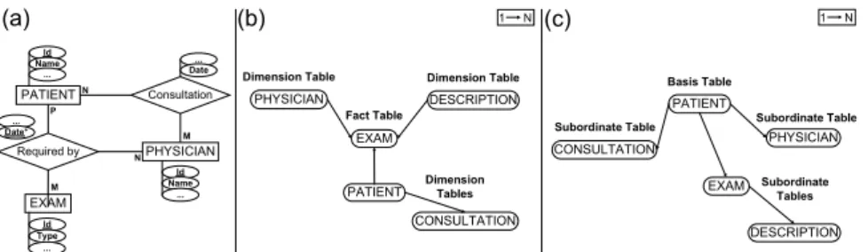
PATIENT PHYSICIAN EXAM Consultation Required by M N M N P Id Name Id Name ... Id Type ... ... Date+ ... ... Date Fact Table PHYSICIAN Dimension Table
PATIENT DimensionTables
DESCRIPTION EXAM Dimension Table CONSULTATION Basis Table PHYSICIAN Subordinate Table PATIENT Subordinate Table DESCRIPTION EXAM Subordinate Tables CONSULTATION (a) (b) 1 N (c) 1 N
Fig. 1. An example comparing DW and the "wagging" process. (a) an Entity-Relation diagram of a Hospital Medical Record Database; (b) a snow-flake schema of the same database in the context of DW; (c) a hierarchical schema of the same database in the context of the "wagging" process
Figure 1 shows an example comparing the DW and the wagging process to analyze a simple Hospital Medical Record database, to mine information about the patients. Figure 1(a) shows an Entity-Relationship diagram of the original database, which is composed by five tables: Patient, Physician, Exam Description, Consultation and Exam. Figure1(b) shows how this database is structured to be analyzed by a DW process, whereas figure 1(c) shows how this database is structured to be mined over patient information using the wagging process. As it can be seen, the N:M cardinality
involved in the database are explored in different ways by both approaches. In the same way, the target of each approach is different. The DW purpose is to analyze the database from the perspective of the set of exams, treating each occurrence as a transaction, regardless the details of each exam, physician or patient - the DW approach compels the analyst to try different details manually, changing the projections of the respective dimension. The wagging approach is more flexible, because it allows different targets to be chosen. In figure 1(c) it was chosen to put the target over the patient table. After the wagging process, any data mining and visualization process can proceed automatically, with the mining process analyzing many different combinations of details to mine the required information.
4. The Proposed Framework
Every visualization and data mining process must receive one table (or data file) as input. Therefore, before data from multiple database relations could be processed, an operational table has to be created. This section describes the proposed wagging process aiming to use visualization to interactively prepare data from multiple relational tables to be submitted to other mining process. Without loss of generality, we assume that the data to be processed is a set of objects with a homogeneous representation, and that part of its data are stored in a relational database table, called the basis relation B. Conceivably, the basis table stores details from objects of only one kind, so other objects referred by this table have their details stored in a set of other tables in the same database, called the subordinate relations Si. If the analysis
process uses data from the basis and subordinate relations, they must be joined to create the operational relation R, which is submitted to the visualization and data mining processes. That is, the visualization and data mining processes receive an operational relation R that is created using the information stored in the set of relations {B, {Si}}.
Considering that a database relation can be defined as a subset of the Cartesian Product of the domains of their attributes, the operational table R can be defined as the join of:
• the basis relationB = {Bi | Bi∈ B}and
• one or more subordinate relations Si = {Sij | Sij∈ Si}.
Once the basis relationB is chosen, it’s necessary to specify the join conditions Jk
between it and a subordinate relation Si not selected yet, or between a subordinate
relation already selected and a subordinate relation not selected yet. Each join condition Jk can involve more than one attribute of each joined relations, that is, a join
condition is the non-empty set
Jk(E, F,ck)={ck=<EθF> | E∈ E, F∈ F}+, E, F ∈ {B, {Si}},
where θ is a comparison operation defined in the domain of the attributes E and F. It is important to note that, starting with the basis relation B, the subordinate relations are being joined one at a time, so that there is only one path from B to each Si.
The operational relation R is created using selected attributes from B and aggregate functions over selected attributes of each Si, that is,
R=Jl( Jk({Ba, Bb, ...| Ba, Bb∈B}, { Agr(Sid), Agr(Sie) , ...| Sid, Sie,∈Si}, (Bc θSif |Bb∈B,
Sif∈Si), { Agr(Sjg), Agr(Sjh) , ...| Sjg, Sjh,∈Sj}, (Bp θSjq |Bp∈(B ∪ Si), Sjq∈Sj)),...
where Ba, Bb,... are attributes of the basis relation, and Sid, Sie,... Sjg, Sjh,... are attributes
from the subordinate relations Si, Sj,... which are joined to the basis relation (or to the
previously joined relations) through the join conditions Jk, Jl,... The subset of
attributes Sid from the subordinate relations generates aggregate Agr(Sid) attributes that
are included in the operational relation R. The aggregation functions are the usual ones provided by the database management system, such as summation SUM, average AVG, minimum MIN, maximum MAX and count COUNT. More than one function can be applied to each attribute of the subordinate relations. For example, parameter measured by a medical exam in the example database can be reported at the relation R by its minimum, maximum and average values for each patient.
After the selection of the aggregate attributes from the subordinate relations, the operational relation R is materialized through the join conditions, and is therefore ready to be submitted to the visualization and data mining processes. The relation R can include attributes from many relations, but every attribute are directly related to the objects described by the basis relation B used to start the process. Not every attribute would be used in the further analysis steps, so the required ones should be selected now. The selection of attributes and the further analysis processes are executed iteratively, but as the operational relation R is materialized, no more time is spent to redo the expensive joins, which otherwise would be necessary. After the further analysis steps, when the important attributes were already determined, the full joins (not using the aggregation functions) can be redone to complete the data mining process. Using the proposed technique, the join operations are executed just twice: once to create the relation R, and once to create the final full table. Otherwise, the joins must be repeated at each iteration step of the analysis process.
This approach results in an operational relation with many attributes, originated from the aggregate attributes of the subordinate relations. This can overload the further analysis processes, so it is interesting to reduce the quantity of attributes submitted to them. Therefore, after the operational relation has been materialized, the user is required to select some attributes, in a selection pre-analysis process. This selection is submitted to a visualization process, and the user is required to interpret the data visualized, confirming that it has enough information for the intended data analysis. If the information is not enough, a new selection is required.
The wagging approach has the following advantages over the conventional processes:
• reduced processing time to generate the operational relation R. As many attributes are aggregated in a single join operation, the need of other join operation when the previously selected attributes shows to be not useful is eliminated. Without the operational relation R, a freshly operational relation must be created after each analysis step iteration;
• support to the user in the preparation process. As the selection of attributes to be submitted to further analysis processes is supported by visual tools, the user now has a fast method to verify the usefulness of the attributes chosen, and do not need to rely exclusively on the semantic of the data he/she already knows.
5 The FastMapDB tool
The FastMapDB tool was developed using the concepts presented in the previous section and the mapping algorithm FastMap [23]. This tool was designed intending to help the user on the process of visual data analysis from data stored in relational databases as a three-dimensional model. It was developed aiming to enable the user to “see” the data distribution, regardless any intrinsic data spatial property. It allows, for example, to verify the existence of outliers, to assist on the steps of data cleaning and pre-processing, and to help the user to choose reduced sets of attributes as input to mine.
The next steps are followed to obtain an operational relation to be visualized in the FastMapDB tool, that are further submitted to data mining processes.
1. Select the database; 2. Select the basis relation B;
3. Select one or more subordinate relations Si and the respective aggregation
functions that should be submitted to the visualization or data mining process; 4. Materialize the operational relation R;
5. Select attributes from R to create the distance function d() for the FastMap algorithm;
6. Define parameters to generate the visualization; 7. Generate and interact with the visualization.
These steps are executed sequentially by the miner analyst. It’s possible to return to any previous step, however, when steps 1 and 2 are re-executed, the data of subsequent steps are discarded.
The initial steps are guided by the tool. First, the available databases are displayed. After the database has been chosen, its relations are shown, and the basis relation B is selected. FastMapDB then presents the attributes from the selected relation, and allows the user to select what Bi attributes to include in the operational relation. After
that, it allows the user to execute steps 3 to 6 iteratively and interactively.
Subordinate relations are chosen in step 3. For each subordinate relation Si, the
user must indicate the attribute(s) of the join condition Jk, the attributes to be included
from Si in relation R, and the aggregation function to be applied over each attribute
(sum, average, minimum, maximum and/or count). After every required subordinate relation have been included, the operational relation R is materialized as a persistent relation in step 4. Therefore, the cost of joins is reduced reusing the already processed table in several visualizations running the join just once.
In step 5 the attributes of the relation R are chosen to build a distance function. The system uses a Lp_norm distance function2 to generate a 3-dimensional spatial
representation of the tuples in the relation, so the user can visualize them. The attributes used by the distance function can be of any type, including numbers, texts (where the LEdit function is used to calculate the attribute differences in the Lp_norm)
2 A L
p distance function of two arrays X(x1, x2, ...xN) and Y(y1, y2, ...yN) is expressed as
or dates (where the number of days between two dates is used), and can be weighted, normalized, and/or used in linear or logarithmic scales. In step 6 the attributes of the operational relation are used to define parameters for the visualization, like using continuous attributes to define the size of the dots, to classify the tuples using colors and shapes, and to select tuples to visualize.
Finally, in step 7 the resultant visualization can be explored and interactively manipulated through operations as rotation, zoom and translation.
5.1 Experimental Evaluation
This section shows the results of applying the FastMapDB tool on real world data sets. The data used for the experiments came from a real Hospital Medical Record database that stores the events in a schema similar to the one presented in Figure 1(a) (the detailed schema is not presented due to confidentially requirements of the hospital). The experiments highlight the gain of performance obtained by the wagging approach. They were performed on a Pentium III 800MHz computer under the MS Windows 2000 operating system, and using an Oracle 8i database server.
5.1.2 Evaluating the Performance
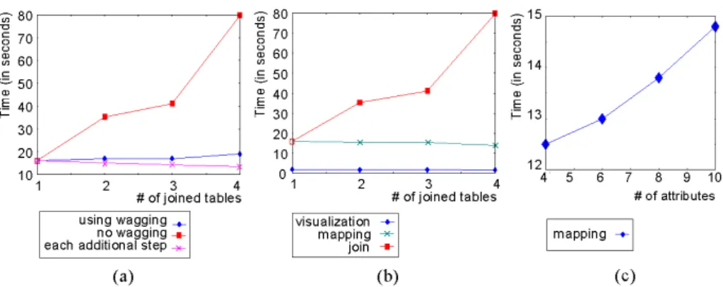
Fig. 2. Evaluating the performance of FatMapDB. (a) total time to join a basis relation with 0 to 3 subordinate relations and visualize 10 attributes from the resulting attributes of the operational relation; (b) time spent by join, mapping and visualization operations without using the wagging process; (c) time spent by FastMapDB varying the number of mapped attributes
The first experiment evaluates the time spent by the FastMapDB tool, varying the number of tables joined. In this experiment we have used a basis relation plus none, one, two, and three subordinate tables using inner joins, which resulted on operational relations of 19287, 18545, 17816 and 16854 tuples respectively. We considered that an operational relation is used by the subsequent processes many times. Thus the experiment measured total time to prepare the operational relation, both using the wagging process, and not using it. The experiment was performed measuring the average of 11 sets of selection, mapping and visualization operations of 10 attributes
out of an operational relation with 11attributes. The results of this experiment are shown at Figure 5 (a). This figure also shows the time required to perform each additional set of selection, mapping and visualization operations. The smaller times obtained using increasing numbers of subordinate relations at each set of operations are due to the use of inner joins, which can reduce the number of tuples in the resulting table, and thus the processing times for the mapping and visualization operations. Figure 5 (b) shows the time spent by each join, mapping and visualization operations that result in the total time to prepare the operational relation without using the wagging process shown in Figure 5 (a).
Figure 5 (c) shows the results of another experiment, where the FastMapDB tool was applied just at the operational table resultant of the join of 2 relations - the basis and one subordinate relation, resulting in 18545 tuples. In this experiment, the performance of the tool was measured varying the number of attributes mapped from 4 to 10 out of an operational relation consisting of 11 attributes. As before, the values shown are the average of 11 executions.
6 Conclusions
In this paper we presented the wagging approach, aiming to prepare operational relations for visualization and data mining processes from a set of relations. These processes require the data to be structured in only one relation (or data file), so the preparation of the data to be submitted to them is a process usually considered as part of the pre-processing steps of the KDD. The preparation of the data from more than one original relation requires time-consuming join operations, and as the whole KDD iterates through every step, much time is spent with these operations. The wagging process creates one operational relation that includes attributes from one basis relation - the target of the KDD process - and attributes calculated as aggregate functions of attributes from one or more subordinate relations. This operational relation enables the data mining and visualization steps of the KDD process to perform several iteration cycles without need to return to the pre-processing step, effectively reducing the overall processing time.
Another benefit of the wagging process is that even the pre-processing can be aided by a visual tool, using the operational relation itself as it is being constructed, to guide the miner analyst during the inclusion of new relations in the operation relations. For the best of the authors' knowledge, this is the first interactive support provided for the data integration step of KDD processes so far.
These concepts enabled the creation of the FastMapDB tool, which includes resources to interactively visualize selections from an operational relation, and uses these resources to aid in the wagging process of create operation relations.
This paper also includes experiments to measure the time required to visualize relations submitted to data mining processes, both using and not using the wagging process. The results show impressive gains in performance, achieving reduction to less than 25% of the time needed when not using the wagging process in typical relations (in this case, joining four relations of ~20,000 tuples into a relation consisting of 10-20 attributes).
References
1. Han, J. and M. Kamber, Data Mining - Concepts and Techniques. 1st Edition ed. 2000, New
York: Morgan Kaufmann Publishers. 550.
2. Keim, D.A. and H.-P. Kriegel, Visualization Techniques for Mining Large Databases: A
Comparison, in IEEE Trans. on Knowledge and Data Engineering. 1996, IEEE Computer Society. p. 923- 938.
3. Becher, J.D., P. Berkhin, and E. Freeman. Automating Exploratory Data Analysis for
Efficient Data Mining. in 6th ACM SIGKDD Int'l Conf. on Knowledge Discovery and Data Mining. 2000. Boston, MA, USA: ACM Press.
4. Traina, C., Jr., et al. Fast feature selection using fractal dimension. in XV Brazilian
Database Symposium. 2000. João Pessoa - PA - Brazil.
5. Smyth, P. and D. Wolpert. Anytime Exploratory Data Analysis for Massive Data Sets. in 3rd
Int'l Conf. on Knowledge Discovery and Data Mining (KDD-97). 1997. California, USA: AAAI Press.
6. Derthick, M., J. Kolojejchick, and S.F. Roth. An Interactive Visualization Environment for
Data Exploration. in 3rd Int'l Conf. on Knowledge Discovery and Data Mining (KDD-97). 1997. California, USA: AAAI Press.
7. Wong, P.C., Visual Data Mining, in IEEE Computer Graphics and Applications. 1999. p.
20-21.
8. Hinneburg, A., D.A. Keim, and M. Wawryniuk, HD-Eye: Visual Mining of
High-Dimensional Data. IEEE Computer Graphics and Applications, 1999. 19(5): p. 22-31.
9. Kanth, K.V.R., D. Agrawal, and A.K. Singh. Dimensionality Reduction for Similarity
Searching in Dynamic Databases. in ACM Int'l Conference on Data Management
(SIGMOD). 1998. Seattle, Washington, USA: ACM Press.
10. Anderson, T.W., An Introduction to Multivariate Statistical Analysis. 1984, New York.
11. Johnson, R.A. and D.W. Wichern, Applied Multivariate Statistical Analysis. 1982, London:
Prentice-Hall.
12. Harman, H.H., Modern Factor Analysis. 1967: University of Chicago Press.
13. Torgenson, W.S., Multidimensional Scaling: I. Theory and Methods. 1952, Psychometrika.
p. 401-419.
14. Kruskal, J.B. and M. Wish, Multidimensional Scaling. 1978, SAGE Publications: Beverly
Hills.
15. Young, F., Multidimensional Scaling: History, Theory, and Applications. 1987, Lawrence
Erlbaum Associates: Hillsdale, NJ.
16. Faloutsos, C. and K.-I.D. Lin. FastMap: A Fast Algorithm for Indexing, Data-Mining and
Visualization of Traditional and Multimedia Datasets. in ACM Int'l Conference on Data Management (SIGMOD). 1995. Zurich, Switzerland: Morgan Kaufmann.
17. Inmon, W.H., Building the Data Warehouse. 1992, New York: John Wiley & Sons.
18. Elmasri, R. and S.B. Navathe, Data Warehousing and Data Mining, in Fundamentals of