its Applications in Machine Learning
Yang Kang
Submitted in partial fulfillment of the requirements for the degree
of Doctor of Philosophy
in the Graduate School of Arts and Sciences
COLUMBIA UNIVERSITY 2017
Yang Kang All Rights Reserved
Distributionally Robust Optimization and its Applications in Machine Learning
Yang Kang
The goal of Distributionally Robust Optimization (DRO) is to minimize the cost of running a stochastic system, under the assumption that an adversary can replace the underlying baseline stochastic model by another model within a family known as the distributional uncertainty region. This dissertation focuses on a class of DRO problems which are data-driven, which generally speaking means that the baseline stochastic model corresponds to the empirical distribution of a given sample.
One of the main contributions of this dissertation is to show that the class of data-driven DRO problems that we study unify many successful machine learning algorithms, including square root Lasso, support vector machines, and generalized logistic regression, among others. A key distinctive feature of the class of DRO problems that we consider here is that our distributional uncertainty region is based on optimal transport costs. In contrast, most of the DRO formulations that exist to date take advantage of a likelihood based formulation (such as Kullback-Leibler divergence, among others). Optimal transport costs include as a special case the so-called Wasserstein distance, which is popular in various statistical applications.
The use of optimal transport costs is advantageous relative to the use of divergence-based formulations because the region of distributional uncertainty contains distribu-tions which explore samples outside of the support of the empirical measure, therefore explaining why many machine learning algorithms have the ability to improve gen-eralization. Moreover, the DRO representations that we use to unify the previously mentioned machine learning algorithms, provide a clear interpretation of the so-called
alization error. As we establish, the regularization parameter corresponds exactly to the size of the distributional uncertainty region.
Another contribution of this dissertation is the development of statistical method-ology to study data-driven DRO formulations based on optimal transport costs. Using this theory, for example, we provide a sharp characterization of the optimal selection of regularization parameters in machine learning settings such as square-root Lasso and regularized logistic regression.
Our statistical methodology relies on the construction of a key object which we call the robust Wasserstein profile function (RWP function). The RWP function similar in spirit to the empirical likelihood profile function in the context of empirical likelihood (EL). But the asymptotic analysis of the RWP function is different because of a certain lack of smoothness which arises in a suitable Lagrangian formulation.
Optimal transport costs have many advantages in terms of statistical modeling. For example, we show how to define a class of novel semi-supervised learning esti-mators which are natural companions of the standard supervised counterparts (such as square root Lasso, support vector machines, and logistic regression). We also show how to define the distributional uncertainty region in a purely data-driven way. Precisely, the optimal transport formulation allows us to inform the shape of the dis-tributional uncertainty, not only its center (which given by the empirical distribution). This shape is informed by establishing connections to the metric learning literature. We develop a class of metric learning algorithms which are based on robust optimiza-tion. We use the robust-optimization-based metric learning algorithms to inform the distributional uncertainty region in our data-driven DRO problem. This means that we endow the adversary with additional which force him to spend effort on regions of importance to further improve generalization properties of machine learning
algo-In summary, we explain how the use of optimal transport costs allow construct-ing what we call double-robust statistical procedures. We test all of the procedures proposed in this paper in various data sets, showing significant improvement in gen-eralization ability over a wide range of state-of-the-art procedures.
Finally, we also discuss a class of stochastic optimization algorithms of indepen-dent interest which are particularly useful to solve DRO problems, especially those which arise when the distributional uncertainty region is based on optimal transport costs.
List of Figures v
List of Tables vi
1 Introduction 1
1.1 How to choose the discrepancy and why? . . . 4
1.2 How to choose the uncertainty region size δ? . . . 9
1.3 On shaping U using data and new statistical insights . . . 12
1.4 How to solve data-driven DRO problem? . . . 15
1.5 Further Discussion . . . 16
2 Robust Wasserstein Profile Inference (RWPI) 17 2.1 Introduction . . . 18
2.1.1 RWPI for optimal regularization of square-root Lasso . . . 18
2.1.2 A broad perspective of the contributions of this chapter . . . . 24
2.1.3 Connections to related inference literature . . . 26
2.1.4 Some connections to Distributionally Robust Optimization and Optimal Transport . . . 28
2.1.5 Organization of this chapter . . . 31
2.2 The Robust Wasserstein Profile Function . . . 31
2.2.2 The RWP Function for Estimating Equations and Its Use as an
Inference Tool . . . 32
2.2.3 The dual formulation of RWP function . . . 35
2.2.4 Asymptotic Distribution of the RWP Function . . . 36
2.3 Distributionally Robust Estimators for Machine Learning Algorithms 42 2.3.1 Dual form of the DRO formulation (2.15) . . . 45
2.3.2 Distributionally Robust Representations . . . 46
2.4 Using RWPI for optimal regularization . . . 49
2.4.1 Linear regression models with squared loss function . . . 52
2.4.2 Logistic Regression with log-exponential loss function . . . 54
2.4.3 Optimal regularization in high-dimensional square-root Lasso 56 2.5 Conclusion . . . 58
3 Sample-out-of-Sample (SoS) Inference 102 3.1 Introduction . . . 103
3.2 Basic Definitions and Main Results . . . 110
3.2.1 SoS Function for Means . . . 110
3.2.2 SoS Function for Estimating Equations . . . 113
3.2.3 Plug-in Estimators for SoS Functions . . . 118
3.3 Methodological Development . . . 124
3.3.1 The Dual Problem and High-Level Understanding of Results . 124 3.3.2 Proof of Theorem 3.1 . . . 128
3.3.3 Proofs of Additional Theorems . . . 146
3.4 Application to Stochastic Optimization and Stress Testing . . . 157
3.5 Conclusions and Discussion . . . 165
mization 168
4.1 Introduction . . . 169
4.2 Alternative Semi-supervised Learning Procedures . . . 173
4.3 Semi-supervised Learning based on DRO . . . 175
4.3.1 Revisit the optimal transport discrepancy: . . . 175
4.3.2 Solving the SSL-DRO formulation: . . . 176
4.4 Error Improvement of Our SSL-DRO Formulation . . . 181
4.5 Numerical Experiments . . . 184
4.6 Discussion on the Size of the Uncertainty Set . . . 185
4.7 Conclusions . . . 188
5 Distributionally Robust Groupwise Regularization Estimator 202 5.1 Introduction . . . 203
5.2 Optimal Transport and DRO . . . 207
5.2.1 Revisit the optimal transport discrepancy . . . 207
5.2.2 DRO Representation of GSRL Estimators . . . 208
5.3 Optimal Choice of Regularization Parameter . . . 210
5.3.1 Revisit The Robust Wasserstein Profile Function . . . 211
5.3.2 Optimal Regularization for GSRL Linear Regression . . . 213
5.3.3 Optimal Regularization for GR-Lasso Logistic Regression . . . 214
5.4 Numerical Experiments . . . 216
5.5 Conclusion and Extensions . . . 219
6 Data-Driven Optimal Transport Cost Selection for Distributionally Robust Optimization 231 6.1 Introduction . . . 232
6.3 Data-Driven Selection of Optimal Transport Cost Function . . . 241
6.3.1 Revisiting Optimal Transport Distances and Discrepancies . . 241
6.3.2 On Metric Learning Procedures . . . 242
6.4 Data Driven Cost Selection and Adaptive Regularization . . . 248
6.5 Robust Optimization for Metric Learning . . . 250
6.5.1 Robust Optimization for Relative Metric Learning . . . 250
6.5.2 Robust Optimization for Absolute Metric Learning . . . 252
6.6 Solving Data Driven DRO Based on Optimal Transport Discrepancies 255 6.7 Numerical Experiments . . . 260
6.8 Conclusion and Discussion . . . 262
7 Discussion and Conclusion 269 7.1 Distributionally Robust Multi-task training . . . 269
7.2 Distributionally Robustness and Robustness in Statistics . . . 271
7.3 Conclusion . . . 272
Bibliography 274
2.1 Figure for RWP function intuition. . . 23
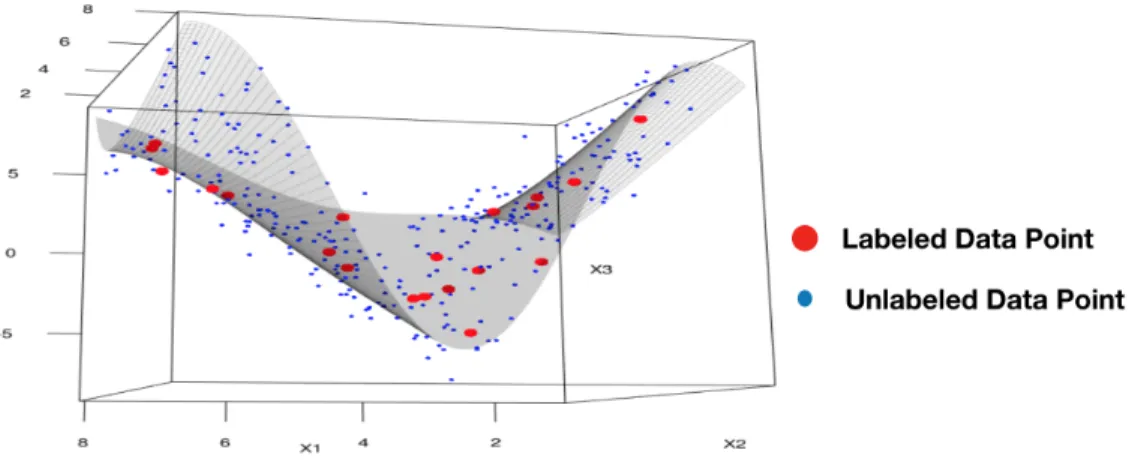
4.1 Figure for motivation of semi-supervised learning. . . 169
4.2 Figure for how SSL-DRO method improve performance. . . 183
5.1 Figure for RWP function of DRO Group Lasso. . . 212
6.1 Figure for illustrating information on robustness. . . 237
6.2 Figure for illustrating the need for data-driven cost function. . . 240
6.3 Figure for apply metric learning to learn data-driven cost for DRO. . 246
2.1 Table for numerical results of RWPI: Sparse regression with d = 300
predictors. . . 100
2.2 Table for numerical results of RWPI: Sparse regression with d = 600 predictors. . . 101
2.3 Table for numerical results of RWPI: Coveraging probability of the worst-case expected loss for sparse regression. . . 101
2.4 Table for numerical results of RWPI: Diabetes data example. . . 101
3.1 Table for SoS inference on CVaR example with Gaussian Data. . . 165
3.2 Table for SoS inference on CVaR example with Laplace Data. . . 166
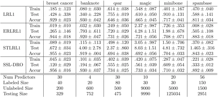
4.1 Table for numerical experiments for SSL-DRO. . . 185
5.1 Table for DRO groupwise regularization with simulated examples for linear model. . . 218
5.2 Table for DRO groupwise regularization with simulated examples for logstic regression model. . . 218
5.3 Table for DRO groupwise regularization with breast cancer data. . . . 218 6.1 Table for DRO with data-driven cost function with real data examples. 261
I wish to express my most sincere thanks to Dr. Jose Blanchet. He is the ideal supervisor that I can imagine before I start my Ph.D. study. Jose has unlimited energy and enthusiasm for exploring and working on research while he is extremely patient and skillful in instructing and inspiring his students. As the old saying in China, “Give a man a fish, and you feed him for a day. Teach a man to fish, and you feed him for a lifetime.”, I could still remember when I start working on research, Jose gave me a baby project to teach me how to explore, come up with meaningful questions, and solve the problems in a proper scientific way. Jose knew the solution to the baby project in advance and utilized as an instructive example to work on research systematically. This is only one of the examples, among many, I benefit from working with Jose. In additional to being a great supervisor, he is more like a godfather and like a friend. His great passions in life and his deep love to his family shows me a great successful role model of finding an optimal work-life balance. I believe it is god’s will that leads me to Jose. It is with his consistent and generous support that I can have a great Ph.D. life in the past four years both in academia study and everyday life in New York. I also would like to appreciate Jose’s family, Lalli, Martin, and Victoria. Without their kind support and understanding, Jose could hardly spend that much time working and exploring with us.
I would like to express my greatest appreciation to my committee members. I could still remember the time when Dr. Richard Davis (former director of the graduate
the Ph.D. program. I took the offer within an hour, and after four years I have proved that I was making the optimal decision. It is under Richard’s administration that the department is becoming stronger and stronger. Dr. Paul Galsserman was also my committee of the oral exam, thanks to his thoughtful question of suggestions, we can complete some further promising research works in the last few months of my Ph.D. study. Dr. Peter Orbanz, who is my neighbor, is more than a friend rather than a supervisor. I appreciate for his time chatting with me at statistics lounge on research and everyday life. I first know Dr. Daniel Hsu from taking his class of Advanced Machine Learning, actually, that was one of the primary reasons that I would like to move my research focus to machine learning then. A lot of intuitions and motivations for my current research was learned from Daniel’s class.
One of the greatest things I love Columbia is the great supportive help from the faculties members and staff of Department of Statistics and also Department of Industrial Engineering and Operations Research. First, I would like to thank Dood Kalicharan. Dood is like the mother of the department, and she helps me taking care of most of everything of my life at Columbia. She is like the angel that God sends to me. When I have the troubles of housing, application for the visa, teaching, graduating... she always says “No worries, let us fix it now!” and help me solve all the problems efficiently. I would like to show special appreciation for Dr. Mark Brown, for his supportive encouragement and instructive suggestions. I also thank Dr. Tian Zheng, for the opportunity staying and presenting in her study group during the past four years, from which I learned a lot to gain intuitions and ideas for this dissertation. In additional, I would give my gratitude to the other faculties members, Dr. Zhiliang Ying, Dr. Yang Feng, Dr. Jingcheng Liu, Dr. Arian Maleki, Dr. Garud Iyengar, Dr. Mark Brown, Dr. Victor de la Pena, Dr. Henry Lam, among others,
help from the other staff members at Department of Statistics and IE&OR, without their support I would have suffered much more during my Ph.D. student life. I also appreciate my supervisors, Dr. Fabio Mercurio and Dr. Gordon Ritter, during my summer internship studies. Their in-depth knowledge and a comprehensive view of the industry have a great impact on me both for my academic research and career development.
I am very grateful for being part of an active research group. I would like to thank Dr. Karthyek Murthy, Fan Zhang, Yanan Pei, Zhipeng Liu, Lin Chen, Fei He, and Chris Dolan for the motivative discussions on research and hard efforts for your joint research work. I would like to thank all my friends during my Ph.D. study, Jing Wu, Xiaopei Zhang, Ji Xu, Xiaowei Tan, Fengpei Li, Swapnil Sahai, Julia Yang, Haolei Weng, Lu Meng, Sihan Huang, Chaai Wu, Yilong Zhang, Zhangyi Hu, Fan Zhang, Karthyek Murthy, Jiqun Tu, Morgane Austern, among others, for their kind help and support. They made the years long Ph.D. study life enjoyable and colorful.
Finally, I would like to thank my parents, Hong Gao and Yong Kang, and my grandparents, Yongyu Gao and Jingsheng Fu, for their unconditional love and en-couraging support. It is their more than twenty years education that makes me here, without them, I could hardly imagine how could I suffer the tough times and reach each goal. I would appreciate the support from the rest of my family, Christina, Jeanna, Mei, Yuan, and David.
Chapter 1
Introduction
Distributionally Robust Optimization (DRO) refers to a class of optimization prob-lems in which the objective is to minimize the cost of running a stochastic system, under the assumption that an adversary can replace the underlying baseline stochas-tic model by another model within a family known as the distributional uncertainty region. More specifically, letl(w, β)be a realized cost when a decisionβ is taken and some (stochastic outcome w) occurs. Consider a stochastic optimization problem of the form
min
β EP∗[l(W, β)], (1.1)
where W ∼ P∗ (the symbol ∼ reads “follows the distribution P”) and EP∗ is used
to denote the expectation with respect to (w.r.t.) the probability measure P∗. The DRO formulation for Equation (1.1) is
min
β maxP∈U EP [l(W, β)], (1.2) where we denoteU as the distributional uncertainty set of this DRO problem (which is composed of probability models which govern the distribution ofW). The intuition
is that P∗ is not fully known and therefore it makes sense to choose β taking into account such ambiguity in our knowledge of P∗. DRO has been actively studied in past decades, see for example Scarf et al. [1958]; Ben-Tal and Nemirovski [1998]; Shapiro and Kleywegt [2002]; Iyengar [2005]; Calafiore and Ghaoui [2006]; Erdoğan and Iyengar [2006]; Delage and Ye [2010]; Goh and Sim [2010]; Bertsimaset al.[2010]; Ben-Talet al. [2010]; Becker [2011]; Dupačová and Kopa [2012]; Ben-Talet al.[2013]; Wiesemann et al. [2014]; Bertsimas et al. [2013]; Wang et al. [2016b]; Peyré et al.
[2016]; Lam and Zhou [2017], and has found applications in areas such as finance and risk management (see in Calafiore [2007]; Lam and Zhou [2015]; Hall et al. [2015]; Glasserman and Yang [2016]), and machine learning (see for example Ruckdeschel [2010]; Zhu and Fukushima [2009]; Zymler [2010]; Shafieezadeh-Abadehet al. [2015]; Blanchetet al. [2016b]; Blanchet and Kang [2017b,a]), among others.
The goal of this dissertation is to develop a comprehensive statistical methodology for data-driven DRO formulations such as (1.2). By data-driven DRO we understand that U is informed by empirical samples Dn = {Wi}ni=1 of the underlying model P∗ (which is unknown). A natural way to incorporate this information is to parameterize the “center” of U using the empirical measure Pn = n−1
Pn
i=1δ{Wi}(dw). Moreover,
we shall introduce a notion of discrepancy between any two probability measures P and Q and we will denote such discrepancy by Dc(P, Q). Using this notation, we
then let
U =Uδ(Pn) = {P :Dc(P, Pn)≤δ}.
In pursuit of the stated goal, this dissertation sets as its objective to answer the following questions:
A) How to choose the discrepancy measure Dc and what are the advantages of
B) How to choose the size of the uncertainty region, δ?
C)Is there a way to inform the shape of the uncertainty regionU in a data-driven way (not only through its center)?
D) Does the method generate new statistical insights?
E)What are the computational challenges that formulations such as (1.2) exposes, and how to address them?
F)Finally, what type of future extensions can be envisioned by this new method-ology?
Throughout the rest of this Introduction, we provide a summary which explains how these questions are addressed in this dissertation and also we provide forward references to the chapters in which our discussion about these questions is elaborated. We will introduce the optimal transport cost and briefly discuss the reason for se-lecting the optimal transport in Section 1.1, this addresses the pointA)and partially point C). In Section 1.2, we address B), there we discuss the role of uncertainty set size δ via making connection to regularization parameters. Then we introduce an optimality criterion, rooted in statistical principles, for choosing δ. In order to optimally evaluate δ, we introduce two classes of inference procedures, which we call RWPI (Robust Wasserstein Profile Inference) and SoS (Sample-out-of-Sample) infer-ence. In Section 1.3, we explore the flexibility of choosing optimal transport costs. We discuss by a judicious choice of such optimal transport cost, we can generate novel learning methods; for example semi-supervised learning. This discussion in Section 1.3 addresses the question D) and E). We discuss briefly the challenges and intro-duce our algorithm to solve data-driven DRO problems directly in Section 1.4, which addresses E). We discuss the potential future applications of our developments, for example, in multi-task learning in Section 1.5; this addresses point F).
1.1
How to choose the discrepancy and why?
Most of the DRO formulations that exist to date take advantage of likelihood based constructions, such as φ−divergence-based discrepancy measures, Calafiore [2007]; Ben-Talet al.[2010, 2013]; Hu and Hong [2013]; Klabjanet al.[2013], which take the form
D(P, Q) =EQ[φ(dP(X)/dQ(X))],
for a strictly convex function satisfying φ(1) = 0. For example, if you take φ(·) =
−log (·), this is known as Kullback-Leibler divergence. For our data-driven DRO formulation, U is centered the empirical measure, i.e. Q = Pn. The definition of
φ−divergence discrepancy requires P to be absolute continuous w.r.t. Pn. In simple
words, the support of P must be a subset of the support of Pn. This constrain on
the support of the elements inside the uncertainty region U can potentially diminish the power of the DRO formulation, specially in statistical applications in which it is important to enhance out-of-sample performance.
In this dissertation we advocate the use of optimal transport based discrepan-cies. We would show via some examples that our choice of optimal transport cost as discrepancy recovers some popular algorithms in machine learning which have been studied and whose out-of-sample performance has been widely tested empirically. However, before we discuss such examples, let us introduce the concept of optimal transport cost or optimal transport discrepancy.
Introducing Optimal Transport Costs
An optimal transportation cost is also known as an earth moving distance in the image processing literature (see in Rubner et al. [1998, 2000]; Rubner and Tomasi [2001]; Wanget al. [2016a] ). Intuitively speaking, as its name suggests, the optimal transport costDc(P, Q)is measuring the cheapest way of rearranging (i.e.
transport-ing the mass of ) distribution P into the distribution Q, where the cost for moving a unit from location u tow is defined as c(u, w).
Normally, we assume the cost function c : Rd+1 ×
Rd+1 → [0,∞] is lower
semi-continuous and we assume c(u, w) = 0 if and only if u = w. Given two probability distributions P(·) and Q(·), with supports SP ⊆ Rd+1 and SQ ⊆Rd+1, respectively,
one can define the optimal transport discrepancy (or optimal transport cost) between P and Q, denoted by Dc(P, Q), as Dc(P, Q) = min π Eπ[c(U, W)] :π ∈ P Rd+1×Rd+1 , πU =P, πW =Q . (1.3) We denoteP Rd+1×
Rd+1 to be set of joint probability measuresπ supported on a
subset of Rd+1×
Rd+1, and πU and πW denote the marginals of U and W under π,
respectively.
In addition to what we stated for the cost function above, if c(·) is symmetric, (i.e. c(u, w) = c(w, u)) and there exist % ≥ 1 such that the triangle inequality holds for c1/%(·), i.e.
c1/%(u, w)≤c1/%(u, v) +c1/%(v, w), for all u, w, v ∈ Rd+1, it can be easily verified that D
c(P, Q)1/% is a metric for
prob-ability measures supported on Rd+1; this corresponds to the Wasserstein metric of order % (see Villani [2003, 2008] for basic properties of optimal transport costs and other metric properties).
For example, if c(u, w) = ku−wk22, where k·k2 is the Euclidean distance in Rm,
semi-continuous and it satisfies the triangle inequality. In that case, D1/2 c (P, Q) = inf q EπkU−Wk 2 2 : π ∈ P(R m× Rm), πU =P, πW =Q
coincides with the Wasserstein distance of order 2.
Wasserstein distances metricize weak convergence of probability measures under suitable moment assumptions, and have received immense attention in probability theory (see Rachev and Rüschendorf [1998a,b]; Villani [2008] for a collection of classi-cal applications). More recently, optimal transport metrics and Wasserstein distances are being actively investigated for its use in various machine learning applications as well (see Seguy and Cuturi [2015]; Peyréet al.[2016]; Rolet et al.[2016]; Solomon et al. [2015]; Frogner et al. [2015]; Srivastava et al. [2015] and references therein for a growing list of new applications).
We can observe that optimal transport discrepancies can be obtained via solving a linear programming problem. For example, let us consider a special case, where Q=Pn and we restrict the support of P, i.e. S(P), to be finite, then, we have that
Dc(P, Pn)is obtained by computing min π X u∈SP X w∈Dn c(u, w)π(u, w) : (1.4) s.t. X u∈SP π(u, w) = 1 n ∀w∈ Dn X w∈DN π(u, w) =P ({u}) ∀ u∈ XN, π(u, w)≥0 ∀ (u, w)∈ SP × Dn
For the general case (i.e. the case in whichUandW are supported in arbitrary subsets of Rd+1), a completely analogous linear program (LP), albeit an infinite dimensional
one, can be defined. Such an infinite dimensional LP has been extensively studied in great generality in the context of Optimal Transport under the name of Kantorovich’s problem (see in Villani [2008]). Requiring c(·) to be lower semi-continuous guaran-tees the existence of an optimal solution to Kantorovich’s problem. Requiring that c(u, w) = 0 if and only if u=wimplies that Dd(P, Q) = 0 if and only if P =Q.
In order to motivate the choice of optimal transport cost as a reasonable selection for data-driven DRO. We now explain discuss how, by choosingc(·)judiciously we can recover some well-known statistical learning methods which improving generalization (i.e. out-of-sample) performance.
Let consider a linear regression mode of the form
Y =β∗TX+e,
whereβ∗ is the true regression parameter and eis the independent mean zero random error. We assume the predictors areX ∈RdandY ∈
Ris the response. Moreover, we
have a collection of data samplesDn={(Xi, Yi)} n
i=1. A standard statistical approach is to use least squares, which consists in consider the problem
min β EPn h Y −βTX2i= min β n −1 n X i=1 Yi−βTXi 2 , where Pn(dx, dy) = n−1 n X i=1 δ{(Xi,Yi)}(dx, dy).
However, as it has been argued in most of the statistical learning textbooks (for example Friedman et al. [2001]; Bishop [2006]; James et al. [2013]; Goodfellow et al. [2016]), when the sample size is relative small relative to the dimension of the problem, direct use of least squares estimation will lead to overfitting and therefore
to poor generalization properties.
In order to enhance the generalization properties of the standard least squares es-timator, let us consider a DRO formulation based on optimal transport discrepancies. We consider the cost function
c (x, y),(u, v)= kx−uk2∞, if y=v ∞, otherwise. . (1.5)
This cost functionc(·)assigns infinite cost wheny6=v, the minimization in Equa-tion (1.3) is effectively over the joint distribuEqua-tions that do not alter the marginal distributions of Y. As a consequence, the resulting neighborhood set Uδ(Pn) =
{P :Dc(P, Pn)≤δ} admits distributional ambiguities only with respect to the
pre-dictors X. Intuitively, we are imposing a certain consistency property in which we predictors which are close should share the same response. Not allowing uncertainty inY may be more sensible in cases in which Y is a categorical variable.
By taking the cost function as in Equation (1.5), we can show that the data-driven DRO formulation for linear regression is equivalent to the square-root Lasso (SR-Lasso) estimator, min β P:Dcmax(P,Pn)≤δ q E(Y −XTβ)2 = min β v u u t 1 n n X i=1 (Yi−XiTβ) 2 +√δkβk1 .
SR-Lasso was introduced by Belloni et al. [2011] as a generalization of the Lasso method (see Tibshirani [1996]). It turns out that SR-Lasso has the benefit that the optimal choice of regularization parameter is free of the magnitude of the variance of the random error. This is particularly appearning in high dimension settings in
which the estimation of the error variance magnitude may be noisy.
A similar data-driven DRO representation could also be made for regularized logistic regression and support vector machine (SVM), among others, as we shall discuss in Chapter 2 Section 2.3. We also discuss futher generalizations, for example, we will establish explicit connections to Group Lasso and adaptive Lasso estimators. These connections will be discussed in Chapter 5 and Chapter 6.
These regularized estimators have been wildly studied and they have been shown empirically to be highly effective in improving generalization performanc. We believe that the explicit connection to a wide range of successful regularization estimators studied in this dissertation makes a strong case for the use of data-driven DRO with optimal transport costs.
1.2
How to choose the uncertainty region size
δ
?
Let us consider the data-driven DRO for general statistical learning model with loss functionl(·), cost functionc(·)and W = (X, Y) for Equation (1.2), which is
min
β Dc(maxP,Pn)≤δ
EP [l(X, Y;β)]. (1.6)
The distributional uncertainty set,Uδ(Pn) = {P :Dc(P, Pn)≤δ}, represents the class
of models that are, in some sense, plausible variations ofPn. For every selectionP in
Uδ(Pn), there is an optimal choiceβ=β(P)which minimizes the risk EP [l(X, Y;β)].
We shall defineΛn(δ) = {β(P) :P ∈ Uδ(Pn)}to be the set of plausible selections of
the parameter β.
Now, for the definition of Λn(δ) to be sensible, we must have that the estimator
is established with the aid of a min-max theorem in Chapter 2, min β∈Rd max P:Dc(P,Pn)≤δ E P [l(X, Y;β)] = min β∈Λn(δ) max P:Dc(P,Pn)≤δ E P [l(X, Y;β)].
Then, we will say thatβ∗ isplausiblewith(1−α)confidence, or simply,(1−α) -plausible ifδ is large enough so thatβ∗ ∈Λn(δ)with probability at least 1−α. This
definition leads us to the optimality criterion that we shall consider.
Our optimal selection criterion for δ is formulated as follows: Choose
δ > 0 as small as possible in order to guarantee that β∗ is plausible with (1−α) confidence.
As an additional desirable property, we shall verify that ifβ∗ is(1−α)-plausible, then Λn(δ)is a (1−α)-confidence region for β∗.
Let us focus our discussion on linear regression model. In order to formally setup an optimization problem for the choice ofδ >0, note that for any givenP, by convex-ity, any optimal selection β is characterized by the first order optimality condition, namely,
EP
Y −βTXX =0. (1.7)
We then introduce the following object, which is the RWP (Robust Wasserstein Pro-file) function associated with the estimating equation (1.7),
Rn(β) = inf
Dc(P, Pn) :EP
Y −βTXX =0 .
Finally, we claim that the optimal choice of δis precisely the1−αquantile, χ1−α,
of Rn(β∗); that is
χ1−α = inf
To see this note that if ˜δ > χ1−α then indeed β∗ is plausible with probability at least
1−α, but ˜δ is not minimal. In turn, note that Rn(β) allows to provide an explicit
characterization of Λn(χ1−α),
Λn(χ1−α) ={β :Rn(β)≤χ1−α}.
Moreover, we clearly have
P (β∗ ∈Λn(χ1−α)) = P(Rn(β∗)≤χ1−α) = 1−α,
soΛn(χ1−α) is a (1−α)-confidence region for β∗.
In order to further explain the role of Rn(β∗), let us define Popt(β∗) to be the set
of probability measures, P, supported on a subset of Rd×
R for which (1.7) holds
with β =β∗. Formally, Popt(β∗) := P :EP Y −β∗TXX =0 .
In simple words,Popt(β∗)is the set of probability measures for which β∗ is an optimal
risk minimization parameter. Observe that using this definition we can write
Rn(β∗) = inf{Dc(P, Pn) :P ∈ Popt(β∗)}.
Consequently, the set
{P :Dc(P, Pn)≤Rn(β∗)}
denotes the smallest uncertainty region aroundPn (in terms ofDc) for which one can
find a distributionP satisfying the optimality condition EP
(Y −βT
∗X)X
=0. In summary,Rn(β∗)denotes the smallest size of uncertainty that makesβ∗
plausi-ble. If we were to choose a radius of uncertainty smaller thanRn(β∗), then no
probabil-ity measure in the neighborhood will satisfy the optimalprobabil-ity conditionEP
(Y −βT
∗X)X
=
0. On the other hand, if δ > Rn(β∗), the set
P :EP (Y −β∗TX)X =0, Dc P, Pn ≤δ
is nonempty. Given the importance ofRn(β∗)in the optimal selection of the
regular-ization parameterλ, it is of interest to analyze its asymptotic properties as n → ∞.
This discussion provides an intuitive understanding for how to pick the uncertainty sizeδforUδ(Pn)optimally using the linear regression example as a motivation. A more
in-depth study of the RWP function is given in Chapter 2 and further applications to machine learning settings are given in Chapter 5. Further extensions to settings in which the support of the elements in the distributional uncertainty are restricted are studied in Chapter 3 and in Chapter 4.
1.3
On shaping
U
using data and new statistical
in-sights
One of the main advantages of considering an optimal transport discrepancy is that we have the flexibility to select a cost function which is either informed by our learning goal or which encodes additional information to improve the generalization perfor-mance.
For example, suppose that we have collection of dataDn ={(Xi, Yi)} n
i=1 and also assume that we have unlabeled observations (i.e. observations without response Y),
which we denote as UN−n ={Xi}Ni=n+1. For simplicity, we consider binary
classifica-tion problem and the responseY ∈ {−1,+1}. Let us further denote the set
EN−n=UN−n× {−1,+1}={Xi,1} N
i=n+1∪ {Xi,−1} N i=n+1,
in which we replicate each unlabeled data point twice, recognizing that the missing label could be any of the two available alternatives. We assume that the data must be labeled either -1 or +1. We then construct the set XN = Dn∪ EN−n which, in
simple words, is obtained by just combining both the labeled data and the unlabeled data with all possible labeles which can be assigned. For a standard empirical risk minimization learning problem of the form,
min
β EPn[l(X, Y;β)],
we can define the semi-supervised learning DRO via
min
β P∈P(XNmax),Dc(Pn,P)≤δ
EP [l(X, Y;β)]. (1.8)
We will argue that by solving the data-driven DRO problem in Equation (1.8), we may enhance the generalization error because we are using the unlabeled data to restrict the support of the members of the distributional uncertainty. The intuition is that if the predictors lie in a lower dimensional subspace of Rd, then it suffices to
enhance the out-of-sample performance of the estimator only on such lower dimen-sional space, which in turn might be well described by the unlabeled data set ifN is sufficiently large.
The semi-supervised learning approach that we advocate in Equation (1.8) is not a robustification method that provide data-driven DRO formulation to any existing
semi-supervised learning algorithm. We provide a different and novel semi-supervised learning approach. Our semi-supervised DRO formulation utilizes the flexibility of the optimal transport discrepancy to encode the unlabeled information into the risk minimization. Further details will be discussed in Chapter 4.
In addition to restricting the support of the elements in the distributional un-certainty set, we are able to choose cost function which adapts to our learning goal. We will show that, by defining a groupwise cost function, we are able to inform the distributional uncertainty regionUδ(Pn)with the side information for predictors and
build up DRO representation for some popular groupwise shrinkage estimators, for example, square-root Group Lasso for linear regression and group-Lasso for logistic regression. The details of the data-driven DRO groupwise regularization estimator will be discussed in Chapter 5.
The groupwise regularization connection is based on having prior assumptions (or side-information) on the predictors. If there is no prior information available, we would like to design the cost function in a fully data-driven approach. We propose a methodology which learns such a distributional uncertainty neighborhood in a natural data-driven way. For example, we consider a parametric family of cost functions of the formc(u, w) = (u−w)TΛ (u−w) for a positive definite Λ. This choice corresponds to the so-called Mahalanobis distance. We use results from the literature on metric learning procedures to calibrate Λ in a way that is consistent with the learning task at hand. This discussion is given in Chapter 6.
Moreover, we also contribute to the metric learning literature by providing a data-driven robust optimization methodology to calibrateΛ. This additional layer of robustification, which then is used when solving our data-driven DRO formulation, justifies the name doubly robust data-driven DRO (DD-R-DRO). The DD-R-DRO methodology is also discussed in Chapter 6.
1.4
How to solve data-driven DRO problem?
For some of the data-driven DRO formulations, the dual formulation is not as easily accessible as in the case of regularized estimators as square-root Lasso, regularized logistic regression, and SVM. As we shall discussed in Chapter 4 and Chapter 6, the data-driven DRO with loss function l(X, Y, β) and cost function c(·), is equivalent to solving min β P:Dcmax(P,Pn)≤δ EP [l(X, Y, β)] = min β minλ≥0 1 n n X i max u {l(u, v, β)−λc((Xi, Yi),(u, v)) +λδ},
where the inner-most optimization (involving maxu) is taken for each sample point
Xi, Yi.
We provide a smoothing approximation technique to remove the inner maximiza-tion over u and propose an unbiased gradient estimation for the stochastic gradient algorithms to the data-driven DRO problem directly. The details of the algorithms and the smoothing approximation bound are discussed in Chapter 4 and Chapter 6. The proposed computational algorithm makes the data-driven DRO formulation applicable rather generally (beyond the setting of standard regularized estimators for which we obtain the representations discussed earlier). The optimization algorithm that we shall discuss is based on stochastic gradient descent, which is scalable to massive data sets.
1.5
Further Discussion
For the data-driven DRO formulation introduced in Section 1.1 and Section 1.3, we note that our data-driven DRO formulations can be applied to more general machine learning algorithms. Once the loss function and its gradient are accessible, we are able to apply our stochastic gradient based algorithm discussed in Chapter 6, to solve the data-driven DRO problem directly.
This is to say, even for a complex model, once the cost function is chosen properly, we can apply data-driven DRO to address the overfitting problem and to improve generalization performance. For example, as we shall discuss in Chapter 7, Section 7.1, we use multi-task training as an example to show that data-driven DRO might help in building novel learning methods to improve the generalization performance.
In Chapter 7, Section 7.2, we include a discussion on difference and connections between robustness in classical statistics and robustness in our DRO formulation. Finally, we will close the dissertation by discussing further potential research avenues, in Chapter 7, Section 7.3,
Chapter 2
Robust Wasserstein Profile Inference
(RWPI)
In this chapter, we introduce RWPI (Robust Wasserstein-distance Profile-based In-ference - pronounced similar to Rupee. The acronym RWPI is chosen to sound just as “RUPI”, where “u” as in put and “i” as in bit. In turn, RUPI means beautiful in Sanskrit.), a novel class of statistical tools which exploits connections between Em-pirical Likelihood, Distributionally Robust Optimization and the Theory of Optimal Transport (via the use of Wasserstein distances). A key element of RWPI is the so-called Robust Wasserstein Profile function, whose asymptotic properties we study in this chapter. We illustrate the use of RWPI in the context of machine learning algorithms, such as the square-root Lasso (Least Absolute Shrinkage and Selection) and regularized logistic regression, among others. For these algorithms, we show how to optimally select the regularization parameter without the use of cross validation. The use of RWPI for such optimal selection requires a suitable distributionally robust representation for these machine learning algorithms, which is also novel and of in-dependent interest. Numerical experiments are also given to validate our theoretical
findings.
2.1
Introduction
The goal of this chapter is to introduce and investigate a novel inference methodology which we call RWPI (Robust Wasserstein-distance Profile-based Inference). RWPI combines ideas from three different areas: Empirical Likelihood (EL), Distributionally Robust Optimization, and the Theory of Optimal Transport. While RWPI can be applied to a wide range of inference problems, in this chapter we use several well known algorithms in machine learning to illustrate the use and implications of this methodology.
We will explain, by means of several examples of interest, how RWPI can be used to optimally choose the regularization parameter in machine learning applications without the need of cross validation. The examples of interest that we study in this chapter include square-root Lasso (Least Absolute Shrinkage and Selection) and regularized logistic regression, among others. In order to explain RWPI let us walk through a simple application in a familiar context, namely, that of linear regression.
2.1.1
RWPI for optimal regularization of square-root Lasso
Consider a given a set of training data Dn ={(Xi, Yi)}ni=1. The input Xi ∈ Rd is a
vector of d predictor variables, and Yi ∈ R is the response variable. It is postulated
that
Yi =β∗TXi+ei,
for someβ∗ ∈Rdand errors {e
1, ..., en}. Under suitable statistical assumptions (such
estimat-ing β∗. Underlying there is a general loss function,l(x, y;β), which we shall take for simplicity in this discussion to be the quadratic loss, namely, l(x, y;β) = y−βTx2
. Over the last two decades, various regularized estimators have been introduced and studied. Many of them have gained substantial popularity because of their good empirical performance and insightful theoretical properties, (see, for example, Tib-shirani [1996] for an early reference and Friedman et al. [2001] for a discussion on regularized estimators). One such regularized estimator, implemented, for example in the “flare" package, see Liet al.[2015], is the so-called square-root Lasso estimator; which is obtained by solving the following convex optimization problem inβ,
min β∈Rd np EPn[l(X, Y;β)] +λkβk1 o = min β∈Rd v u u t 1 n n X i=1 l(Xi, Yi;β) +λkβk1 , (2.1)
where kβkp denotes the p-th norm in the Euclidean space. The parameter λ, com-monly referred to as the regularization parameter, is crucial for the performance of the algorithm and it is often chosen using cross validation.
2.1.1.1 Distributionally robust representation of square-root Lasso We shall illustrate how to choose λ, satisfying a natural optimality criterion, as the quantile of a certain object which we call the Robust Wasserstein Profile (RWP) func-tion evaluated at β∗. This will motivate a systematic study of the RWP function as the sample size, n, increases. However, before we define the associated RWP func-tion, we first introduce a class of representations which are of independent interest and which are necessary to motivate the definition of the RWP function for choosing λ.
One of our contributions in this chapter is a representation of (2.1) in terms of a Distributionally Robust Optimization formulation (see Section 2.3). In particular, we construct a discrepancy measure,Dc(P, Q), based on a suitable Wasserstein-type
distance, between two probability measures P and Qsatisfying that
min β∈Rd np EPn[l(X, Y;β)] +λkβk1 o2 (2.2) = min β∈Rd P:Dmaxc(P,Pn)≤δ EP [l(X, Y;β)],
where δ = λ1/2. Observe that the regularization parameter is fully determined by the size of the uncertainty,δ, in the distributionally robust formulation on the right hand side of (2.2).
The setUδ(Pn) ={P :Dc(P, Pn)≤δ}is called the uncertainty set in the language
of distributionally robust optimization, and it represents the class of models that are, in some sense, plausible variations ofPn. The estimator obtained by solving Equation
(2.2) is referred as distributionally robust regression estimator, and we remark that this notion of robustness is different from the standard statistical robustness which primarily addresses data contamination with outliers (see Huber [1964]).
For every selection P in Uδ(Pn), there is an optimal choice β = β(P) which
minimizes the risk EP [l(X, Y;β)]. We shall define Λn(δ) ={β(P) :P ∈ Uδ(Pn)} to
be the set of plausible selections of the parameter β.
Now, for the definition of Λn(δ) to be sensible, we must have that the estimator
obtained from the left hand side of (2.2) is plausible. This follows from the following result, which is established with the aid of a min-max theorem in Section 2.4,
min
Then, we will say thatβ∗ isplausiblewith(1−α)confidence, or simply,(1−α) -plausible ifδ is large enough so thatβ∗ ∈Λn(δ)with probability at least 1−α. This
definition leads us to the optimality criterion that we shall consider.
Our optimal selection criterion for δ is formulated as follows: Choose
δ > 0 as small as possible in order to guarantee that β∗ is plausible with (1−α) confidence.
As an additional desirable property, we shall verify that ifβ∗ is(1−α)-plausible, thenΛn(δ)is a (1−α)-confidence region forβ∗. A computationally efficient procedure
for evaluating Λn(δ) will be studied in future work. Our focus in this chapter is on
the optimal selection of δ.
2.1.1.2 The associated Robust Wasserstein Profile Function
In order to formally setup an optimization problem for the choice of δ >0, note that for any given P, by convexity, any optimal selection β is characterized by the first order optimality condition, namely,
EP
Y −βTXX =0. (2.3)
We then introduce the following object, which is the RWP function associated with the estimating equation (2.3),
Rn(β) = inf
Dc(P, Pn) :EP
Y −βTXX =0 . (2.4)
of Rn(β∗); that is
χ1−α = inf
z :P (Rn(β∗)≤z)≥1−α .
To see this note that if ˜δ > χ1−α then indeed β∗ is plausible with probability at least
1−α, but ˜δ is not minimal. In turn, note that Rn(β) allows to provide an explicit
characterization of Λn(χ1−α),
Λn(χ1−α) ={β :Rn(β)≤χ1−α}.
Moreover, we clearly have
P (β∗ ∈Λn(χ1−α)) = P(Rn(β∗)≤χ1−α) = 1−α,
soΛn(χ1−α) is a (1−α)-confidence region for β∗.
In order to further explain the role of Rn(β∗), let us define Popt(β∗) to be the set
of probability measures, P, supported on a subset of Rd×
R for which (2.3) holds
with β =β∗. Formally, Popt(β∗) := P :EP Y −β∗TX X =0 .
In simple words,Popt(β∗)is the set of probability measures for which β∗ is an optimal
risk minimization parameter. Observe that using this definition we can write
Consequently, the set
{P :Dc(P, Pn)≤Rn(β∗)}
denotes the smallest uncertainty region aroundPn(in terms ofDc) for which one can
find a distribution P satisfying the optimality condition EP
(Y −βT
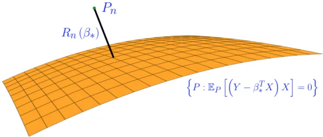
∗X)X
=0, see Figure 2.1 for a pictorial representation of Popt(β∗) and Rn(β∗).
Figure 2.1: Illustration of RWP function evaluated at β∗
In summary,Rn(β∗)denotes the smallest size of uncertainty that makesβ∗
plausi-ble. If we were to choose a radius of uncertainty smaller thanRn(β∗), then no
probabil-ity measure in the neighborhood will satisfy the optimalprobabil-ity conditionEP
(Y −β∗TX)X =
0. On the other hand, if δ > Rn(β∗), the set
P :EP (Y −β∗TX) =0, Dc P, Pn ≤δ
is nonempty. Given the importance ofRn(β∗)in the optimal selection of the
regular-ization parameterλ, it is of interest to analyze its asymptotic properties as n→ ∞. It is important to note, however, that the estimating equations given in (2.3) are just one of potentially many ways in which β∗ can be characterized. In the case
of Gaussian input there is an (well known) intimate connection between (2.3) and maximum likelihood estimation. In general it appears sensible, at least from the standpoint of philosophical consistency to connect the choice of estimating equation with the loss function l(x, y;β) used in the Distributionally Robust Representation (2.2).
2.1.2
A broad perspective of the contributions of this chapter
The previous discussion in the context of linear regression highlights two key ideas: a) the RWP function as a key object of analysis, and b) the role of distributionally robust representation of regularized estimators.
The RWP function can be applied much more broadly than in the context of regularized estimators. This chapter is written with the goal of studying the RWP function for estimating equations generally and systematically. As an application, we showcase the study of the RWP function in a context of great importance, namely, the optimal selection of regularization parameters in several machine learning algorithms. Broadly speaking, RWPI is a statistical tool which consists in building a suitable RWP function in order to estimate a parameter of interest. From a philosophical standpoint, RWPI borrows heavily from Empirical Likelihood (EL), introduced in the seminal work of Owen [1988, 1990]. There are important methodological differences, however, as we shall discuss in the sequel. In the last three decades, there have been a great deal of successful applications of Empirical Likelihood for inference [Owen, 1991; Qin and Lawless, 1994; Bravo, 2004; Hjort et al., 2009; Zhou, 2015]. In principle, all of those applications can be revisited using the RWP function and its ramifications. Therefore, we spend the first part of the chapter, namely Section 2, discussing general properties of the RWP function.
The application of RWPI for the optimal selection of regularization parameters in various machine learning settings is given in Section 2.4. Once a suitable RWP function is obtained, the results in Section 2.4 are obtained directly from applications of our results in Section 2.2. In order to obtain the correct RWP function formulation for each of the machine learning settings of interest, however, we will need to derive a suitable distributionally robust representations which, analogous to those discussed in the square-root Lasso setting. These representations are given in Section 2.3 of this chapter.
We now provide a more precise description of our contributions:
A) We provide general limit theorems for the asymptotic distribution (as the sample size increases) of the RWP function defined for general estimating equations, not only those arising from linear regression problems. Hence, providing tools to apply RWPI in substantial generality (see the results in Section 2.2.4).
B) We explain how, by judiciously choosing Dc(·), we can define a family of
regularized regression estimators (See Section 2.3). In particular, we will show how square-root Lasso (see and Theorem 2.2), and regularized logistic regression (see Theorem 2.3) arise as a particular case of a RWPI formulation.
C) The results in B) allow to obtain the appropriate RWP function to select an optimal regularization parameter. We then illustrate how to analyze the distribution of Rn(β∗) using our results formA) (see Section 2.4).
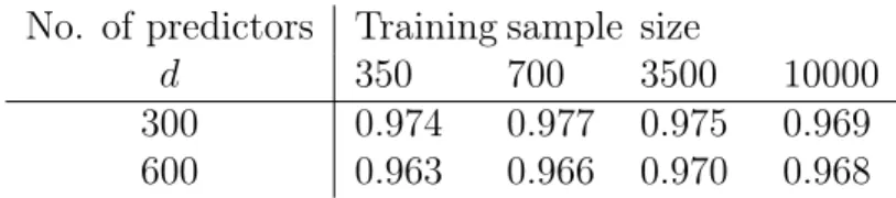
D) We analyze our regularization selection in the high dimensional setting for square-root Lasso. Under standard regularity conditions, we show (see Theorem 2.6)
that the regularization parameter λ might be chosen so that, λ= π π−2 Φ−1(1−α/2d) √ n ,
where Φ−1(·) is the inverse cumulative distribution function of standard normal dis-tribution. The behavior ofλas a function ofnandd is consistent with regularization selections studied in the literature motivated by different considerations.
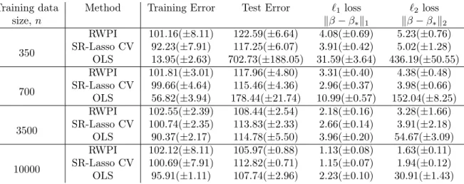
E) We analyze the empirical performance of RWPI for the selection of the op-timal regularization parameter in the context of square-root Lasso. This is done in Appendix 2.D. We apply our analysis both to simulated and real data and compare against the performance of cross validation. We conclude that our approach to-wards regularization parameter selection offers comparable (not worst) performance, although at a much lesser computational cost than cross validation.
We now provide a discussion on topics which are related to RWPI.
2.1.3
Connections to related inference literature
Let us first discuss the connections between RWPI and EL. In EL one builds a Profile Likelihood for an estimating equation. For instance, in the context of EL applied to estimating β satisfying (2.3), one would build a Profile Likelihood Function in which the optimization object is only defined as the likelihood (or the log-likelihood) between a given distribution P with respect to Pn. Therefore, the analogue of the
uncertainty set {P : Dc(P, Pn) ≤ δ}, in the context of EL, will typically contain
distributions whose support coincides with that of Pn. In contrast, the definition of
the RWP function does not require the likelihood between an alternative plausible model P, and the empirical distribution, Pn, to exist. Owing to this flexibility, for
example, we are able to establish the connection between regularization estimators and a suitable profile function.
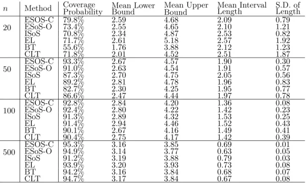
There are other potential benefits of using a profile function which does not restrict the support of alternative plausible models. For example, it has been observed in the literature that in some settings EL might exhibit low coverage Owen [2001]; Chen and Hall [1993]; Wu [2004]. It is not the goal of this chapter to examine the coverage properties of RWPI systematically, but it is conceivable that relaxing the support of alternative plausible models, as RWPI does, can translate into desirable coverage properties.
From a technical standpoint, the definition of the Profile Function in EL gives rise to a finite dimensional optimization problem. Moreover, there is a substantial amount of smoothness in the optimization problems defining the EL Profile Function. This degree of smoothness can be leveraged in order to obtain the asymptotic distribution of the Profile Function as the sample size increases. In contrast, the optimization problem underlying the definition of RWP function in RWPI is an infinite dimen-sional linear program. Therefore, the mathematical techniques required to analyze the associated RWP function are different (more involved) than the ones which are commonly used in the EL setting.
A significant advantage of EL, however, is that the limiting distribution of the associated Profile Function is typically chi-squared. Moreover, such distribution is self-normalized in the sense that no parameters need to be estimated from the data. Unfortunately, this is typically not the case in the case of RWPI. In many settings, however, the parameters of the limiting distribution can be easily estimated from the data itself.
Another set of tools, strongly related to RWPI, have also been studied recently by the name of SOS (Sample-Out-of-Sample) inference as we shall discuss in Chapter 3.
In this setting, also an RWP function is built, but the support of alternative plausible models is assumed to be finite (but not necessarily equal to that of Pn). Instead,
the support of alternative plausible models is assumed to be generated not only by the available data, but additional samples coming from independent distributions (defined by the user). The mathematical results obtained for the RWP function in the context of SOS are different from those obtained in this chapter. For example, in the SOS setting, the rates of convergence are dimension-dependent, which is not the case in RWPI.
2.1.4
Some connections to Distributionally Robust
Optimiza-tion and Optimal Transport
Connection between robust optimization and regularization procedures such as Lasso and Support Vector Machines have been studied in the literature, see Xu et al.
[2009a,b]. The methods proposed here differ subtly: While the papers Xu et al.
[2009a,b] add deterministic perturbations of a certain size to the predictor vectorsX to quantify uncertainty, the Distributionally Robust Representations that we derive measure perturbations in terms of deviations from the empirical distribution. While this change may appear cosmetic, it brings a significant advantage: measuring de-viations from empirical distribution, in turn, lets us derive suitable limit laws (or) probabilistic inequalities that can be used to choose the size of uncertainty, δ, in the uncertainty region Uδ(Pn) = {P :Dc(P, Pn)≤δ}.
Now, it is intuitively clear that as the number of samplesnincrease, the deviation of the empirical distribution from the true distribution decays to zero, as a function of n, at a specific rate of convergence. To begin with, one can simply use, as a direct approach to choosing the size of δ, a concentration inequality that measures
this rate of convergence. Such simple specification of the size of uncertainty, suitably as a function of n, does not arise naturally in the deterministic robust optimization approach. For a concentration inequality that measures such deviations in terms of the Wasserstein distance, we refer to Fournier and Guillin [2015] and references there in. For an application of these concentration inequalities to choose the size of uncertainty set in the context of distributionally robust logistic regression, refer Shafieezadeh-Abadeh et al. [2015]. It is important to note that, despite imposing severe tail assumptions, these concentration inequalities dictate the size of uncertainty to decay at the rate O(n−1/d), where d is the number of covariates. Unfortunately,
this prescription scales non-graciously as the dimension d increases. Since most of the modern learning problems have huge number of covariates, application of such concentration inequalities with poor rate of decay with dimensions may not be most suitable for applications.
In contrast to directly using concentration inequalities, the prescription that we advocate typically has a rate of convergence of orderO n−1/2
as n → ∞ (for fixed d). Moreover, as we discuss in the case of Lasso, according to our results corre-sponding to contribution E), our prescription of the size of uncertainty actually can be shown (under suitable regularity conditions) to decay at rate O(plogd/n) (uni-formly over d and n), which is in agreement with the findings of compressed sensing and high-dimensional statistics literature (see Candes and Tao [2007]; Belloni et al.
[2011]; Negahban et al. [2012] and references therein). Interestingly, the regulariza-tion parameter prescribed by RWPI methodology is automatically obtained without looking into the data (unlike cross-validation).
Although we have focused our discussion on the context of regularized estimators, our results are directly applicable to the area of data-driven Distributionally Robust Optimization whenever the uncertainty sets are defined in terms of a Wasserstein
distance or, more generally, an optimal transport metric. In particular, consider a given distributionally robust formulation of the form
min
θ:G(θ)≤0 P: Dmaxc(P,Pn)≤δ E
P [H(W, θ)],
for a random elementW and a convex function H(W,·) defined over a convex region {θ : G(θ) ≤ 0} (assuming G : Rd →
R convex). Here Pn is the empirical measure
of the sample {W1, ..., Wn}. One can then follow a reasoning parallel to what we
advocate throughout our Lasso discussion.
Argue, by applying the corresponding KKT (Karush-Kuhn-Tucker) conditions, if possible, that an optimal solution θ∗ to the problem
min
θ:G(θ)≤0EPtrue[H(W, θ)] satisfies a system of estimating equations of the form
EPtrue[h(W, θ∗)] = 0, (2.5)
for a suitable h(·) (where Ptrue is the weak limit of the empirical measure Pn as
n → ∞). Then, given a confidence level 1−α, one should choose δ as the (1−α)
quantile of the RWP function function
Rn(θ∗) = inf{Dc(P, Pn) :EP[h(W, θ∗)] = 0}.
The results in Section 2 can then be used directly to approximate the(1−α)quantile of Rn(θ∗). Just as we explain in our discussion of the square-root Lasso example, the selection ofδ is the smallest possible choice for which θ∗ is plausible with (1−α)
confidence.
2.1.5
Organization of this chapter
The rest of the chapter is organized as follows. Section 2.2 deals with contributionA) where we first revisit Wasserstein distances, which we discussed in Chapter 1 Section 1.1, and discuss the Robust Wasserstein Profile function as an inference tool in a way which is parallel to the Profile Likelihood in EL. We derive the asymptotic distribu-tion of the RWP funcdistribu-tion for general estimating equadistribu-tions. Secdistribu-tion 2.3 corresponds to contribution B), namely, distributionally robust representations of some popular machine learning algorithms. Section 2.4 discusses contribution C), namely the use of results from contributions A) for optimal regularization parameter selection. Our high-dimensional analysis of the RWP function in the case of square-root Lasso is also given in Section 2.4. The proofs for the main results along with various technical lemmas and numerical experiments are given in the Appendix.
2.2
The Robust Wasserstein Profile Function
Given an estimating equation EPn[h(W, θ)] = 0, the objective of this section is to
study the asymptotic behavior of the associated RWP function Rn(θ). To do this,
we first introduce some notation to define optimal transport costs and Wasserstein distances. Following this, we provide evidence, initially with a simple example, fol-lowed by results for general estimating equations, that the profile function defined using Wasserstein distances is tractable.
2.2.1
Revisit Optimal Transport Costs and Wasserstein
Dis-tances
Let us revisit the definition and properties of optimal transport discrepancy and Wasserstein Distance in this subsection.
Let c : Rm ×
Rm → [0,∞] be any lower semi-continuous function such that
c(u, w) = 0 if and only if u =w. Given two probability distributions P(·) and Q(·)
supported on Rm, one can define the optimal transport cost or discrepancy between P and Q, denoted by Dc(P, Q), as
Dc(P, Q) = inf
Eπ[c(U, W)] :π ∈ P(Rm×Rm), πU =P, πW =Q . (2.6)
Here, P(Rm×Rm)is the set of joint probability distributions π of(U, W)supported
onRm×Rm, andπU andπW denote the marginals of U andW underπ, respectively.
Throughout this chapter, we shall selectDc for a judiciously chosen cost function
c(·)in formulations such as (2.2). It is useful to allowc(·)to be lower semi-continuous and potentially be infinite in some region to accommodate some of the applications, such as regularization in the context of logistic regression, as we shall see in Section 2.3. So, our setting requires discrepancy choices which are slightly more general than standard Wasserstein distances.
2.2.2
The RWP Function for Estimating Equations and Its
Use as an Inference Tool
The Robust Wasserstein Profile function’s definition is inspired by the notion of the Profile Likelihood function, introduced in the pioneering work of Art Owen in the context of EL (see Owen [2001]). We provide the definition of the RWP function for
estimating θ∗ ∈Rl, which we assume satisfies
EPtrue[h(W, θ∗)] =0, (2.7)
for a given random variable W taking values in Rm and an integrable function h :
Rm ×Rl → Rr. The parameter θ∗ will typically be unique to ensure consistency,
but uniqueness is not necessary for the limit theorems that we shall state, unless we explicitly indicate so.
Given a set of samples {W1, ..., Wn}, which are assumed to be i.i.d. copies of W,
we define the Wasserstein Profile function for the estimating equation (2.7) as,
Rn(θ) := inf
Dc(P, Pn) : EP[h(W, θ)] =0 . (2.8)
Here, recall that Pn denotes the empirical distribution associated with the training
samples {W1, . . . , Wn} and c(·) is a chosen cost function. In this section, we are
primarily concerned with cost functions of the form,
c(u, w) =kw−ukρq, (2.9)
where ρ ≥ 1 and q ≥ 1. We remark, however, that the methods presented here can be easily adapted to more general cost functions. For simplicity, we assume that the samples{W1, . . . , Wn} are distinct.
Since, as we shall see, that the asymptotic behavior of the RWP function Rn(θ)is
dependent on the exponentρ in Equation (2.9), we shall sometimes writeRn(θ;ρ)to
make this dependence explicit; but whenever the context is clear, we dropρ to avoid notational burden. Also, observe that the profile function defined in (2.4) for the linear regression example is obtained as a particular case by selecting W = (X, Y),
β =θ and definingh(x, y, θ) = (y−θTx)x.
Our goal in this section is to develop an asymptotic analysis of the RWP function which parallels that of the theory of EL. In particular, we shall establish,
nρ/2Rn(θ∗;ρ)⇒R¯(ρ). (2.10)
for a suitably defined random variableR¯(ρ) (throughout the rest of the chapter, the symbol “⇒” denotes convergence in distribution).
As the empirical distribution weakly converges to the underlying probability dis-tribution from which the samples are obtained from, it follows from the definition of RWP function in Equation (2.10) that Rn(θ;ρ) → 0, as n → ∞, if and only if θ
satisfiesE[h(W, θ)] =0; for every otherθ,we have thatnρ/2R
n(θ;ρ)→ ∞.Therefore,
the result in (2.10) can be used to provide confidence regions (at least conceptually) around θ∗. In particular, given a confidence level 1−α in (0,1), if we denote ηα as
the (1−α)quantile of R¯(ρ), that is, P R¯(ρ)≤ηα
= (1−α), then ¯ Λn ηα n = n θ :Rn(θ;ρ)≤ ηα n o
yields an approximate(1−α) confidence region forθ∗. This is because, by definition of Λ¯n(ηα/n), we have P θ∗ ∈Λ¯n(ηα/n) =P nρ/2Rn(θ∗;ρ)≤ηα ≈P R¯(ρ)≤ηα = 1−α.
Throughout the development in this section, the dimension m of the underlying random vector W is kept fixed and the sample sizen is sent to infinity; the function h(·) can be quite general. In Section 2.4.3, we extend the analysis of RWP function to the case where the ambient dimension could scale with the number of training
samplesn, in the specific context of square-root Lasso for linear regression.
2.2.3
The dual formulation of RWP function
The first step in the analysis of the RWP function Rn(θ) is to use the definition of
the discrepancy measureDc to rewrite Rn(θ) as,
Rn(θ) = inf
Eπ[c(U, W)] :π ∈ P(Rm×Rm), Eπ[h(U, θ)] = 0, πW =Pn ,
which is aproblem of moments of the form,
Rn(θ) = inf π∈P(Rm×Rm) Eπ[c(U, W)] : Eπ[h(U, θ)] = 0, (2.11) Eπ[I(W =Wi)] = 1 n, i= 1, . . . , n .
The problem of moments is a classical linear programming problem for which the respective dual formulation and strong duality have been well-studied (see, for ex-ample, Isii [1962]; Smith [1995]). The linear program problem over the variableπ in Equation (2.11) admits a simple dual semi-infinite linear program of form,
sup ai∈R,λ∈Rr ( a0+ 1 n n X i=1 ai : a0+ n X i=1 ai1{w=Wi}(u, w) +λ Th(u, θ)≤c(u, w),∀u, w∈ Rm ) = sup λ∈Rr ( 1 n n X i=1 inf u∈Rm c(u, Wi)−λTh(u, θ) ) = sup λ∈Rr ( −1 n n X i=1 sup u∈Rm λTh(u, θ)−c(u, Wi) ) .
Proposition 2.1 below states that strong duality holds under mild assumptions, and the dual formulation above indeed equalsRn(θ).
Proposition 2.1. Let h(·, θ) be Borel measurable, and Ω = {(u, w) ∈ Rm ×
Rm :
c(u, w) < ∞} be Borel measurable and non-empty. Further, suppose that 0 lies in the interior of the convex hull of{h(u, θ) :u∈Rm}. Then,
Rn(θ) = sup λ∈Rr ( −1 n n X i=1 sup u∈Rm λTh(u, θ)−c(u, Wi) ) .
A proof of Proposition 2.1, along with an introduction to the problem of moments, is provided in Appendix 2.B of this Chapter.
2.2.4
Asymptotic Distribution of the RWP Function
In order to gain intuition behind (2.10), let us first consider the simple example of estimating the expectation θ∗ = E[W] of a real-valued random variable W, using h(w, θ) = w−θ.
Example 2.1. (RWPI for mean estimation.) Let h(w, θ) = w−θ with m = 1 = l = r. First, suppose that the choice of cost function is c(u, w) = |u−w|ρ for some ρ > 1. As long as θ lies in the interior of convex hull of support of W, Proposition Equation (2.1) implies,
Rn(θ;ρ) = sup λ∈R ( −1 n n X i=1 sup u∈R λ(u−θ)− |Wi−u| ρ ) = sup λ∈R ( −λ n n X i=1 (Wi−θ)− 1 n n X i=1 sup u∈R λ(u−Wi)− |Wi−u| ρ ) . As max ∆ {λ∆− |∆| ρ}= (ρ−1)|λ/ρ|ρ/(ρ−1),
we obtain Rn(θ;ρ) = sup λ ( −λ n n X i=1 (Wi −θ)−(ρ−1) λ ρ ρ ρ−1) = 1 n n X i=1 (Wi−θ) ρ .
Then, under the hypothesis that E[W] = θ∗, and assuming Var[W] =σ2
W <∞,
we obtain,
nρ/2Rn(θ∗;ρ)⇒R¯(ρ)∼σWρ |N(0,1)|
ρ
,
where N(0,1) denotes a standard Gaussian random variable. The limiting dis-tribution for the case ρ = 1 can be formally obtained by setting ρ = 1 in the above expression for R¯(ρ), but the analysis is slightly different. When ρ= 1,
Rn(θ) = sup λ∈R ( −λ n n X i=1 (Wi−θ)− 1 n n X i=1 sup u∈R λ(u−Wi)− |u−Wi|