Assessing the performance of multiple spectral–spatial features of a hyperspectral image for classification of urban land cover classes using support vector machines and artificial neural network

(1)

Assessing the performance of multiple spectral-spatial features of a

hyperspectral image for classification of urban land cover classes

using support vector machines and artificial neural network

Reddy Pullanagari, R. a*, Gábor Kereszturi a, Ian J. Yule, a, Ghamisi, Pedram ac

a

New Zealand Centre for Precision Agriculture, Soil and Earth Sciences group, Institute of Agriculture and Environment (IAE), Massey University, Palmerston North, Private Bag 11 222, New Zealand

b _{Remote Sensing Technology Institute (IMF), German Aerospace Center (DLR), 82234 Weßling, Germany}_Signal c_{Processing in Earth Observation, Technische Universität München (TUM), 80333 Munich, Germany}

Abstract. Accurate and spatially detailed mapping of complex urban environments is essential for land managers. Classifying high spectral and spatial resolution hyperspectral images is a challenging task because of its data abundance and computational complexity. Land-use classification based on the consideration of spectral information, i.e., without any spatial organization, has limited potential in the final classification map. Consequently, approaches with a combination of spectral and spatial information in a single classification framework have attracted special attention because of their potential to improve the classification accuracy. In this study, we extracted multiple features from spectral and spatial domains of hyperspectral image and evaluated with two supervised classification algorithms such as support vector machines (SVM and artificial neural network (ANN). The spatial features considered in this study are produced by Gray Level Co-occurrence Matrix (GLCM) and extended multi-attribute profiles (EMAP). All of these features were stacked and the most informative features selected using a genetic algorithm-based support vector machine (GA-SVM). After selecting the most informative features, the classification model was integrated with a segmentation map. The segmentation procedure was performed on the hyperspectral image using the Hidden Markov Random Field (HMRF). We tested the proposed method on a real application of hyperspectral image acquired from AisaFENIX and also on widely used hyperspectral images (ROSIS and AVIRIS). From the results, it can be concluded that the proposed framework significantly improves the results with different spectral and spatial resolutions over different instrumentation.

Keywords: Hyperspectral, classification, multiple features, gray level co-occurrence matrix (GLCM), extended multi-attribute profiles (EMAP), and genetic algorithm-based support vector machine (GA-SVM).

* Author, E-mail: [email protected]

1 Introduction

Mapping of urban land cover information is essential to many groups and agencies such as urban planners and policy makers, as classified maps can form a basis for short and long term resource management and planning.

Due to the availability of remote sensing images, a wide range of studies have been conducted which has proven that it can offer accurate and cost-effective information for land

(2)

ASTER) have widely been used in classification studies [4, 5], the classification accuracy was limited due to the small number of spectral bands and their broad spectral and spatial resolution [6]. Consequently, the new generation of satellite sensors such as IKONOS, World View-2 and 3, QuickBird, Orb View-3, and GeoEye, have been launched, which offer enhanced spatial resolution (1-10 m), which enables identification of small urban features. For instance, [6] used WorldView-2 satellite imagery with 8 bands and 2, 4, 10 and 30 m spatial resolutions for mapping urban land cover in Nottingham, UK. The classification accuracy was significantly improved with increased spatial resolution, in which 2 m resolution imagery gained a high overall accuracy (OA) of 90%, while coarser resampled imagery-based classifications obtained OA of 31%. Nonetheless, few ground objects are less separable due to constrained spectral properties.

Hyperspectral sensors were considered as potential tools for mapping urban land-cover classes as they acquire radiance values in many narrow and continuous bands which are the diagnostic absorption or reflection signatures that help to discriminate complex ground features accurately [7]. Studies have proven that urban materials can be more accurately characterized with hyperspectral data compared to multispectral information [8]. Hyperion is a spaceborne hyperspectral mission which offers fine spectral data, but the potential applicability of data is constrained with coarse spatial resolution results preventing recognition of small-scale features in a diverse urban scene. Nevertheless, future hyperspectral satellite missions such as HyspIRI (Hyperspectral Infrared Imager), EnMAP (Environmental Mapping and Analysis Program) [9], and PRISMA, planned to sample on a large spatial extent with high temporal resolution, however, they have limited spatial resolution (30 - 60 m). Consequently, with the advancement of technology, high spatial and spectral resolution airborne sensors such as AVIRIS-NG

(3)

(Airborne Visible-Infrared Imaging Spectrometer - Next Generation) [10], AisaFENIX [11], DAIS, CAO-2 (Carnegie Airborne Observatory-2) [12], APEX [13] to name a few, have been developed which are considered as a valuable data source for detailed thematic urban mapping [14]. In addition to fine spectral data, desirable spatial information with a significant reduction in the number of mixed pixels is possible, which enables detection of small urban features accurately.

Despite these advanced sensor configurations, classifying hyperspectral imagery with high spatial resolution remains challenging due to the large volume of data which leads to computational complexity [13-15]. In particular, the number of training samples is very limited relative to the number of features which carry redundant information. This results in an apparent reduction of classification accuracy. This problem also known as the curse of dimensionality or Hughes phenomenon [16]. Moreover, high spatial resolution can increase intra-class variation due to different ages, and decrease inter-class variation as the majority of the urban materials look spectrally similar, which results uncertainty in classification accuracy [13]. There are several classification algorithms, either parametric or nonparametric, which have been proposed to classify hyperspectral images. In case of urban mapping however, nonlinear nonparametric approaches, such as support vector machines (SVM), random forest (RF), and artificial neural network (ANN), were better suited as the urban data are complex and violate the assumption of statistical distribution [17, 18]. Momeni et al. [6] indicated that SVMs are well suited for mapping urban landscapes when using very high resolution images because they can handle noise present in the training data. SVMs can produce very accurate classification results when there is no balance between dimensionality (number of bands) and the number of available

(4)

class boundaries that commonly exist in the hyperspectral data [19]. However, aforementioned algorithms, to some extent, are sensitive to high-dimensional space (Hughes phenomena). To overcome this problem, a sufficient number of samples are required - but in practice the number of training samples is limited. Therefore, feature extraction (FE) and feature selection (FS) techniques have been proposed to address these issues [20]. An FE technique transforms the high dimensional space (original data) into a lower dimensional subspace which preserves the total variation being present in the original space. The transformation may be linear or nonlinear and supervised or unsupervised. Principal component analysis (PCA) [21], minimum noise fraction (MNF) [22], projection pursuit (PP), independent component analysis (ICA) [23], are widely used linear unsupervised approaches for producing a new sequence of orthogonal images. Class separation can be further optimized using supervised algorithms such as discriminant analysis FE (DAFE) [24], decision boundary FE (DBFE) and nonparametric weighted FE (NWFE) [25]. However, reducing the number of dimensions by FE might lead to a loss of information relevant to the classification scheme and thus results in lower classification accuracy [26]. On the contrary, FS selects an optimal subset of features based on some criteria where discrimination relevant features were selected using training samples and removes unrelated features thereby significant improvement in class separability and classification accuracy.

Although the majority of studies have focused on spectral data to classify hyperspectral images, recent studies have agreed that the fusion of spectral and spatial information significantly improves the classification accuracy. Utilizing the information from high spatial resolution hyperspectral images, studies have attempted to extract the spatial (contextual) features such as morphological features [27, 28], textural features [29], wavelet based spatial indices [30], object based features [31], pixel shape index [32], hidden markov random field

(5)

(HMRF) [21] then combined with spectral data. The concept of morphological profile is based on a simultaneous use of openings and closings on a scalar image with a set of known shapes, also called structural element (SE) [33]. Ak [34] used structural information from the derivative of the morphological profiles (DMP) for a segmentation procedure in which segments were hierarchically modelled based on the factors of spectral homogeneity and neighbourhood information. Although MP and DMP proved as a potential tool for spatial feature extraction, the shape of the SE is fixed. Consequently, an adaptive profile concept of Attribute Profiles (APs) was proposed to overcome this problem which characterizes the image at multiscale thus comprehensive spatial information can be extracted [35]. These APs are extended to hyperspectral images, called as extended attribute profiles (EAPs), by concatenation of MPs which are obtained by applying on sub-space of the original data to reduce ill-posed problems. Individual algorithms or features have a capacity to perform best classification results. However, the classification can be further improved by combining the multiple features with efficient algorithms.

This paper aims to extract multiple features (spectral, textural and EAPs) from high spatial resolution hyperspectral imagery acquired using AisaFENIX sensor on urban landscape. This study considers and integrates the spectral information with textural, morphological, and neighbourhood pixel information to differentiate land cover classes using supervised classification.

2 Methods

With the given recent work, several researchers attempted to incorporate different data types into the classification task and achieved improved accuracy [21, 36]. Efficient combination of data

(6)

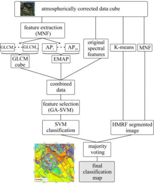
Fig. 1 General scheme of the proposed approach for classifying hyperspectral images

accuracy. Consequently, we attempted to incorporate different spectral and spatial features such as GLCM (Gray level co-occurrence matrix), EMAP (extended multi-attribute profiles) and segmentation map (Fig .1). In addition, optimal features were selected using genetic algorithm (GA) and evaluated with two supervised algorithms such as SVM and ANN.

(7)

2.1 GLCM

GLCM is a widely used method to describe the textural properties of an image, and explains spatial correlation characteristics as well [37]. Image texture indicates the homogenous regions of the image which can be used in segmentation and classification [38, 39]. GLCM is computed based on the spatial distribution of co-occurring pixel brightness (i.e. gray levels), which is a function of distance and angular relationships between two neighbouring pixels. In this study, GLCM was applied on the first ten MNF bands of the hyperspectral image that account for the maximum amount of total variation within the scene. On each MNF image, six different statistical textural features were calculated from co-occurrence matrix: mean, variance, homogeneity, contrast, dissimilarity, entropy, second movement and correlation.

𝐺𝐿𝐶𝑀 𝑚𝑒𝑎𝑛 = 𝜇𝑖𝑗= ∑ ∑ 𝑖𝑗(𝑝(𝑖, 𝑗) 𝑁 𝑗=1 𝑁 𝑖=1 ) 𝐺𝐿𝐶𝑀 𝑉𝑎𝑟𝑖𝑎𝑛𝑐𝑒 = 𝜎𝑖𝑗= ∑ ∑(𝑖 − 𝜇𝑖,𝑗)2𝑝(𝑖, 𝑗) 𝑁 𝑗=1 𝑁 𝑖=1 𝐺𝐿𝐶𝑀 𝐻𝑜𝑚𝑜𝑔𝑒𝑛𝑒𝑖𝑡𝑦 𝐻𝑂𝑀 = ∑ ∑ 1 1 + (𝑖 − 𝑗)2 𝑁 𝑗=1 𝑁 𝑖=1 𝑝(𝑖, 𝑗) 𝐺𝐿𝐶𝑀 𝐶𝑜𝑛𝑡𝑟𝑎𝑠𝑡 𝐶𝑂𝑁 = ∑ ∑ 𝑝(𝑖, 𝑗)(𝑖 − 𝑗)2 𝑁 𝑗=1 𝑁 𝑖=1 𝐺𝐿𝐶𝑀 𝑑𝑖𝑠𝑠𝑖𝑚𝑖𝑙𝑎𝑟𝑖𝑡𝑦 (𝐷𝐼𝑆) = ∑ ∑ 𝑝(𝑖, 𝑗) |𝑖 − 𝑗| 𝑁 𝑗=1 𝑁 𝑖=1 𝐺𝐿𝐶𝑀 𝑒𝑛𝑡𝑟𝑜𝑝𝑦 (𝐸𝑁𝑇) = ∑ ∑ 𝑝(𝑖, 𝑗) log(𝑝(𝑖, 𝑗)) 𝑁 𝑗=1 𝑁 𝑖=1

where p(i, j) indicates the portability of all possible pairs of adjacent pixel gray levels i and j for a distance d and considers four direction angles (𝜃) (0, 45, 90, 135). N is the number of gray levels present in the image constructed under 64 gray level quantization. High level quantization

(8)

window size 3×3 to extract the fine scale statistical parameters listed above from the selected MNF bands (Fig. 1).

2.2 EMAP

Mathematical Morphology (MM) is a well-established theoretical framework proposed to describe geometrical structures of the images based on the theory of lattice algebra, set theory, topology, and integral geometry [41]. In image processing, MM investigates the small patterns or shapes, which are called structural elements (SE), in a given image using basic operations such as dilation and erosion. These operations are considered as building blocks to derive two important transformations, opening and closing. Openings and closings can remove brighter and darker regions while preserving the geometrical characteristics of the structures present in the gray scale image. They are proven to be effective in analysing and extracting spatial information that can consistently improve the classifier performance [20, 35, 42]. Although, MMs and their modifications (e.g., morphological profiles) have been used intensively in the remote sensing community, their concepts have a few limitations such as: (i) the shape of the SE is fixed, and consequently, they cannot efficiently extract spatial information; and (2) SEs are only able to extract information related to the size of existing objects, while they are unable to characterize information related to the gray-level characteristics of the regions [43].

To address these issues, attribute profiles (APs) have been proposed [35]. APs are the advanced version of morphological profiles and are able to extract detailed multilevel characteristics of an image. A sequence of morphological attribute filters (AFs) was applied to a gray-level image by merging its connected components to derive APs. APs are extended to multispectral or hyperspectral data to extract different types of attribute profiles and stacked

(9)

together as EMAP [23]. A comprehensive survey on spectral-spatial classification approaches based on APs has been reported in [8].

Initially, an attribute A is computed for every connected components of a grayscale image f according to a given reference value λ. For each connected component (Ci) of the image, if the A(Ci) > λ, then the corresponding region is kept unaffected, otherwise, it is set to the grayscale value of the adjacent region with the closer, greater or lower value (leading to thinning and thickening profiles). An AP is obtained by applying a sequence of attribute thinning and thickening transformations with a given sequence threshold {λ1, λ2,…, λn}.

AP(f) = {ϕn(f),…..,ϕ1(f), f,γ1(f),….,γn(f)},

where ϕi and γi are the thickening and thinning transformations, respectively, calculated on the

input gray scale image f. Due to the high dimensionality of hyperspectral images and in order to avoid producing redundant features, attribute filtering was suggested to be only applied to the first few features (instead of all the bands) extracted by a feature extraction approach such as MNF, which significantly reduces the computational complexity and CPU processing time [23]. By doing so, one will come up with extended attribute profile (EAP), which can mathematically be given by

EAP = {AP(f1), AP(f2),……,AP(fq)},

where q is the number of MNF components preserved. From the above definition, the APs from each MNF component were combined by concatenating them in a single vector which leads to EMAP (Fig. 2).

In this study, multiple features (reflectance spectra, GLCM and EMAP) were concatenated into one feature vector and fed to the support vector machine (SVM) classifier (Fig. 2).

(10)

2.3 Support vector machines (SVM)

The SVM is a widely used supervised classification method, which does not require any prior assumptions about the statistical distribution of data.

The general idea behind SVM is to differentiate training samples belonging to different classes by tracing maximum margin hyperplanes in the feature space [44]. SVMs were originally introduced to solve linear classification problems, while hyperspectral images are usually nonlinear. To make the SVM well-suited for hyperspectral images, they can be generalized to nonlinear decision functions by considering the so-called kernel trick. A kernel-based SVM is being used to project the pixel vectors into a higher dimensional space and estimate maximum margin hyperplanes in this new space, in order to improve linear separability of data [44]. Among different types of kernels, the Gaussian radial basis function (RBF) has widely been used in remote sensing. This kernel has two parameters. The parameters C (the parameter which controls the trade-off between the maximization of the margin and minimization of classification error) and γ (kernel width) can be tuned using a strategy called grid search with n-fold cross-validation. Here, we used 10-fold cross-validation to tune hyperplane parameters.

Although SVM models can provide good generalization in high–dimensional input spaces, feature selection is important for improving the classification accuracy, to filter out the bands that are irrelevant [45, 46].

2.4 GA-SVM

In order to reduce the dimensionality of the stacked multiple features, a feature selection algorithm was applied to select the best optimal set. In this study, genetic algorithm was used. The GA is a stochastic method which imitates the biological evolution process. This approach has widely been used for search and optimization techniques [47]. GA considers a set of

(11)

randomly chosen chromosomes from the search space to create initial population. Each chromosome is comprised of a sequence of genes where each gene represents one of the spectral bands, and the number of genes being equal to the number of features (n = 638). The total is generated from a combination of GLCM features (n = 80), EMAPs (n = 110) and spectra features (n = 448). The chromosomes are binary-encoded where each gene can assume to be one or zero, in which 1 show the presence of the corresponding band and 0 shows the absence of the corresponding band. The fitness of each chromosome is evaluated by using a fitness function. In this study, SVM classification accuracy was considered to evaluate the better chromosome.

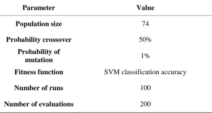
Table 1 Parameter of GA-SVM

The fittest chromosomes have higher probability to reproduce in each generation and aimed to improve overall fitness of the population. New chromosomes as offsprings were introduced in the next generation by performing single-point crossover where two parent chromosomes were split at a random point. After the cross-over, mutation was applied to increase the randomness of the individuals. This algorithm is repeated until the termination criteria are fulfilled. The parameters were presented in Table 2.

Parameter Value

Population size 74

Probability crossover 50%

Probability of

mutation 1%

Fitness function SVM classification accuracy

Number of runs 100

(12)

2.5 Artificial neural network

Artificial neural network (ANN) is a parametric mathematical model to solve complex non-linear classification problems [48]. The concept of ANN is based on the principles of human nervous system. In recent years the use of ANNs has continuously growing in remote sensing community because of its wide range of advantages (i) NN effectively deals with data that do not require normality assumptions (ii) ancillary data and multisource data can be incorporated into model to strengthen the relationships between input and output data (iii) ANNs required less number of training samples when supervised classification is performed. Artificial neurons are represented by nodes and connected using a link called network. There are different NN architectures available to solve supervised classification problems: radial basis function NN (RBF NN), probability NN (PNN), multilayer perceptron (MLP NN). MLPNN is a type of feed forward architecture widely used in remote sensing community [49]. Typically, MLP comprised of input, output and one or more hidden layers, and the adjacent layers are interconnected with neurons or nodes. The number of inputs nodes corresponds to number of bands used in the classification task, while in the output the number corresponds to number of classes. The nodes in the hidden layer contain nonlinear activating functions. These nodes are interconnected by a certain weight and bias which are determined by using training samples and Levenberg-Marquardt optimization [50]. The number of neurons in the hidden layer was optimized by testing different numbers, and the over-fitting of the model avoided by executing early-stopping. The weights between the nodes being adjusted by iteratively calculating the error.

(13)

2.6 Hidden Markov Random Field (HMRF)

Hidden Markov random field (HMRF) is a segmentation procedure, which has been used in medical imaging applications [51] and introduced to use in the remote sensing community by Ghamisi et al. [21]. HMRF is a probability-based modelling technique which considers the spatial information at object scale and preserves the edges information to avoid over-smoothing on boundaries between different classes. In the HMRF framework, initial image segmentation was performed using means clustering on the first component of MNF image. Different k-means clusters were tested on the final classification model. As a result 28 clusters were considered as inputs in the segmentation process. From this, initial labels and parameters were generated for maximum a posteriori (MAP) and expectation maximization algorithms. MAP algorithm iteratively reassigns the class labels based on probability distribution function and neighborhood information. In addition to the segmentation process, edge information was preserved which was extracted using edge detection algorithm. In this study, Sobel edge detection algorithm was applied on the first component of MNF image. For detailed description of HMRF refer to [21].

2.7 Majority voting (MV)

After selecting the features using GA, SVM classification map was created and then fused with the segmented image obtained by HMRF using a procedure called majority voting. In which frequently occurring GA-SVM class labelled pixels in each segmented region were selected using the following equation [51].

𝐶𝐿 (𝑅𝑗) = arg max 𝐾={1,2,…𝑘} 𝑉𝑅_𝑗(𝑘) 𝑉𝑅𝑗 > 𝑟

(14)

where CL(Rj) is the final assigned class label of the segmented region Rj. VRj(k) is the number of

samples labelled as class k within Rj, VRj is the number of all samples within Rj, and r is a

constraint parameter. By using this procedure within a segmented region, spatial errors are significantly minimized.

2.8 Accuracy assessment

A confusion matrix was computed from the results of different classification models which indicate how many pixels were correctly classified in each class. From the confusion matrix, accuracy parameters such as overall accuracy (OA) and kappa coefficient (k) were generated. OA indicates the percentage of pixels correctly classified in each class.

𝑂𝐴 =∑ 𝑁𝑖

𝑝 𝑖

𝑇

where P is the number of classes, Ni is the summation of correctly classified pixels, and T denotes total number of pixels being tested. Kappa coefficient measures the quality of overall classification by comparing the agreement against the one expected by chance [52].

𝑘 =𝑚0− 𝑚𝐶

1 − 𝑚𝐶

Where mo represents the proportion of correct agreement in the validation dataset, and mc is the proportion of agreement that is expected by chance. The possible values range from -1 to + 1, where -1 indicates disagreement and +1 indicates perfect agreement between actual and predicted classes.

(15)

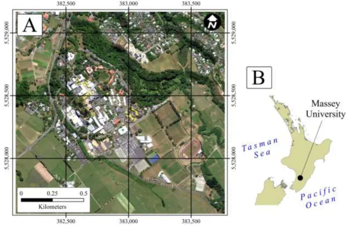
Fig. 2 The study area, Massey University (a) RGB image (b) location

3. Hyperspectral datasets

3.1 Imagery from AisaFENIX

The study was conducted at Massey University (40˚23.156’ S latitude and 175˚37.227’ E longitude) located in the southern part of the city of Palmerston North, New Zealand (Fig.1). The study area comprised of a range complex heterogeneous land cover types such as buildings with different roof materials, roads, sidewalks, vegetation (dairy farms and trees), bare soil, water and playgrounds (Fig. 1).

The AisaFENIX (Specim, Finland) is a full spectrum hyperspectral imaging sensor covering visible to SWIR (380-2500 nm). This sensor has single optics with a single input slit where light

(16)

enters and is dispersed against two focal plane arrays (FPA) using two diffraction gratings optimized for VNIR and SWIR. The focal plane arrays are a 12 bit dynamic range Complementary Metal Oxide Semiconductor (CMOS) and the other is a 16 bit dynamic range cryogenically cooled Mercury Telluride Cadmium (MCT). The FPA image VNIR and SWIR respectively and are used to maximise the sensitivity and signal-to-noise ratio (SNR). AisaFENIX is a pushbroom type sensor which means that the hyperspectral image is created in a line scan fashion by forward motion of the platform. The sensor has a field of view (FOV) of 32.3° and instantaneous field of view of 0.084°. The AisaFENIX used in this study was coupled with RT Oxford Survey+ Global Positioning System (GPS) and Inertial Measurement Unit (IMU) system for accurate registration of the data. During the aerial survey, a spectral binning setting of 4×2 was used in the VIS-NIR to enhance signal strength. No spectral binning was used in the SWIR region.

The raw hyperspectral imagery was corrected for boresight effects due to a misalignment between the IMU and the imaging sensor. The original raw DN data was corrected for bad detector, resulting in horizontal strips in the data. The faulty lines have been detected using statistics from each column of image data, and then replaced by the spectrally neighbour bands’ values. The data have been geometrically and radiometrically calibrated using the CaliGeoPRO software package. The atmospheric corrections were performed on the original scanning geometry (i.e. non-georectified) imagery using flat terrain atmospheric correction method implemented in ATCOR-4 [53]. The atmospheric compensated imagery was then georectified and mosaicked together using ENVI. This mosaicked imagery was smoothed spatially and spectrally to reduce the noisiness of the data cube.

(17)

A total of 23 different land-cover classes were considered in the classification scheme which includes nine different types of roof top, five vegetation types, water, soil and two different shadows (Table 2). Each land-cover class was identified and polygons created using high resolution RGB images and ground survey throughout the study area.

Table 2 The selected land cover classes and the number of pixels in training and validation data sets for AisaFENIX

Class Training pixels Validation pixels

1

Roof tops

Tiles 50 431

2 Metal 40 222

3 New building roof 53 236

4 Roof_1 35 118 5 Roof_2 34 124 6 Roof_3 33 109 7 Roof_4 13 30 8 Roof_5 27 98 9 Roof_6 24 234 10 Manmade structures Pavement 14 38 11 Gravel 31 269 12 Tennis court 26 144

13 Race running track 22 70

14 Road 28 247 15 Bare soil 29 292 16 Vegetation Dairy pasture 50 1914 17 Lawn pasture 40 1545 18 Dried lawn 33 689 19 Bush 35 1060 20 Trees 24 722 21 Water 21 182 22

Shadows Building shadow 19 89

23 Tree shadow 18 83

The pixels in the selected polygons were randomly divided into training and validation datasets. The selected number of pixels in training and validation data corresponding to each land use class is presented in Table 1. A general workflow of the proposed image classification approach is illustrated in Figure 2. Below, we briefly discuss the main building blocks of the

(18)

3.2 Imagery from ROSIS

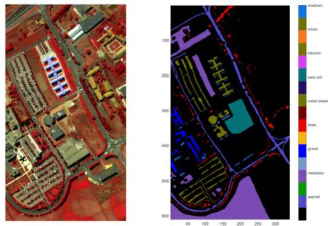
The second hyperspectral data was collected in 2001 by ROSIS optical sensor over the area of the University of Pavia located in Italy. The data has 103 spectral bands in the spectral range of 430 nm to 860 nm. The size of the hyperspectral image is 610×340 pixels with a spatial resolution of 1.3 m. Fig.3a false color composite of ROSIS university of pavia, and Fig.3b shows nine different classes of the image. In this study, a total of 3158 pixels were used for training the models while the remaining pixels were used for testing.

Fig. 3 (a) False color composition of the university of pavia (b) reference map including nine classes.

(19)

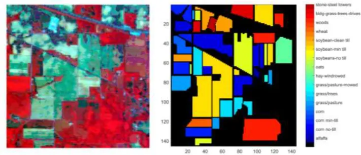
The third hyperspectral data used in this experiment was collected by the AVIRIS (Airborne Visible/Infrared Imaging Spectrometer) over the area of Indian pines region in Northwestern Indiana in 1992. This image comprises 145×145 pixels with 200 spectral bands spanned from 400 to 2500 nm and a spatial resolution of 20 m/pixel. As shown in Fig. 4 the image has 16 classes. In order to perform classification, approximately 10% of random pixels were selected for training which leads to a total of 898 pixels. The remaining pixels allocated for testing.

Fig. 4 (a) False color composition of the AVIRIS Indian pines (b) reference map including sixteen classes.

4 Results

4.1 Results from AisaFENIX

We evaluated the performance of different methods for classifying hyperspectral images collected by AisaFENIX imaging system. A wide range of land-cover classes (n = 23) were

(20)

selected for classification (Table 2), majority of the classes are manmade surfaces (Table 2). Different spectral and spatial related features were extracted from the hyperspectral image.

The classification performance on validation data using SVM and ANN was presented in Table 3 with overall accuracy, k statistic and individual class accuracy. Note that both classifiers achieved highest accuracy when all the features were integrated together.

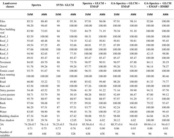
Table 3 Overall classification accuracies (in percent), k statistic and individual class accuracies were obtained for different data types extracted from hyperspectral data acquired from AisaFENIX using support vector machine (SVM) and artificial neural network (ANN).

Land-cover classes Spectra SVM+ GLCM Spectra + GLCM + EMAP GA-Spectra + GLCM + EMAP GA-Spectra + GLCM + EMAP + HMRF

SVM ANN SVM ANN SVM ANN SVM ANN SVM ANN

Tiles 85.51 88.40 85 95.36 97.91 96.06 97.91 98.14 92.84 100.00 Metal 98.20 98.65 98 100.00 100.00 100.00 100.00 100.00 100.00 100.00 New building roof 83.90 72.03 84 72.03 84.75 71.19 70.34 91.10 100.00 100.00 Roof_1 85.59 100.00 98 100.00 98.31 100.00 100.00 100.00 100.00 100.00 Roof_2 55.65 60.48 56 74.19 52.42 50.81 50.81 50.81 100.00 95.45 Roof_3 49.54 97.25 49 92.66 68.81 97.25 67.89 100.00 100.00 100.00 Roof_4 97.06 100.00 100 100.00 100.00 100.00 100.00 100.00 100.00 100.00 Roof_5 94.90 82.65 97 77.55 100.00 100.00 100.00 100.00 42.15 98.00 Roof_6 69.01 85.47 84 85.47 85.47 85.47 85.47 85.47 100.00 100.00 Pavement 84.85 69.70 88 75.76 96.97 90.91 96.97 87.88 84.11 30.19 Gravel 91.76 99.26 95 99.26 97.77 100.00 99.26 93.31 96.14 78.37 Tennis court 93.75 91.67 94 100.00 96.53 100.00 100.00 100.00 100.00 100.00 Race running track 100.00 100.00 100 100.00 100.00 100.00 100.00 100.00 100.00 80.46 Road 66.80 35.22 72 49.80 85.02 99.60 88.26 100.00 81.33 75.77 Bare soil 83.56 100.00 90 100.00 97.26 100.00 100.00 100.00 100.00 100.00 Dairy pasture 54.48 65.52 55 70.06 61.39 91.22 71.16 99.90 94.31 97.70 Lawn pasture 58.71 55.79 58 50.10 88.28 88.03 92.69 86.47 87.00 99.12 Dried lawn 95.79 88.97 96 88.97 96.81 88.97 97.97 91.29 97.11 100.00 Bush 97.04 98.68 97 97.55 99.81 100.00 100.00 100.00 79.52 93.47 Trees 86.29 97.51 87 97.51 93.77 92.94 92.24 96.81 100.00 100.00 Water 83.85 98.90 90 99.45 91.76 100.00 97.25 100.00 100.00 99.45 Building shadow 87.34 76.40 91 67.42 98.88 95.51 98.88 100.00 64.84 36.29 Tree shadow 25.30 39.76 24 12.05 34.94 6.02 30.12 6.02 100.00 100.00 OA 74.28±0.7 78±1.6 76.25±0.5 78±0.6 85.58±0.4 91±1 88.37±0.4 94±0.8 89.04±1.4 94±0.3 k 0.71 0.75 0.73 0.76 0.83 0.90 0.86 0.93 0.88 0.93 Number of variables 448 448 528 528 638 638 96 96 96 96

(21)

However, ANN produced highest overall accuracy (94%) compared to SVM (OA = 90%) (McNemar’s Z score > 1.96). Moreover, with all data types ANN produced better accuracy compared to SVM. When the spectral data alone was used in classification tasks, more number of classes were classified accurately using ANN compared to SVM. From the Table 3, one could say that the addition EMAP features to the spectral data significantly improved the overall accuracy (Mc Nemar’s Z score > 1.96), whereas GLCM features did not significantly improve the accuracy (Mc Nemar’s Z score < 1.96). However, interestingly, the accuracy of few land-cover classes such as roof_2, and tree shadow was decreased. We also report that GA significantly reduced number of features from 638 to 96 and also improved the accuracy levels in both cases (88% ≤ OA ≤ 94%).

A total of 40 features were selected from the domain of EMAP, 53 bands from the spectral domain and 3 features from the domain of GLCM. The selected spectral bands present all over the spectrum from visible to short wave infrared (SWIR) region. From the domain of GLCM, the GLCM contrast (2) and entropy (1) features were selected in the final model. This OA again slightly improved with SVM after applying the segmentation procedure with HMRF where majority of classes were classified with high accuracy (79-100%) except the classes roof_5 (46.15%) and building shadow (65.84%). In contrast, in case of ANN, the accuracy was not improved after fusing with segmentation map, Overall, the results confirm that combining multiple features significantly improved the classification accuracy compared to spectral data alone. Fig. 5 and Fig. 6 show the classification maps using the proposed approach with SVM and ANN.

(22)

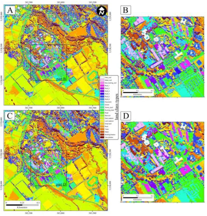
Fig. 5 SVM classification maps based on multiple features Spectra + GLCM + EMAP using GA-SVM (a) before fusing with the segmentation map (c) after fusing with segmentation map.

(23)

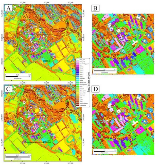
Fig. 6 ANN classification maps based on multiple features Spectra + GLCM + EMAP using GA-SVM (a) before fusing with the segmentation map (c) after fusing with segmentation map.

(24)

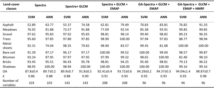
4.2 Results from ROSIS

We also evaluated the proposed method on ROSIS data set. Table 4 shows that the using all features (spectral data, GCLM and EMAP) significantly improved the classification results. Similar to the conclusions of AisaFENIX data, the genetic algorithm optimized the number features from 208 to 96 which lead to the best classification accuracy with both classification algorithms (SVM and ANN). The classification maps using different approaches were illustrated in Fig. 7. We can notice in the Fig. 7, after applying HMRF majority of the classes were classified with distinct boundaries. In the final classification results, all classless were well described (accuracy > 90%) with ANN.

Table 4 Overall classification accuracies (in percent), k statistic and individual class accuracies were obtained for different data types extracted from hyperspectral data acquired from ROSIS using support vector machine (SVM) and artificial neural network (ANN).

Land-cover

classes Spectra Spectra+ GLCM

Spectra + GLCM + EMAP GA-Spectra + GLCM + EMAP GA-Spectra + GLCM + EMAP + HMRF

SVM ANN SVM ANN SVM ANN SVM ANN SVM ANN

Asphalt 52.89 63.77 55.37 74.58 62.81 79.49 70.83 83.81 76.82 91.33 Meadows 76.92 91.88 73.57 91.88 77.09 92.54 85.38 93.91 99.85 99.85 Gravel 97.62 95.83 97.02 95.83 98.81 98.14 99.40 98.82 89.23 96.35 Trees 95.60 97.85 97.80 97.85 98.90 100.00 97.94 97.83 88.77 98.94 Metal sheets 92.31 74.04 98.35 79.82 98.90 83.57 99.45 81.08 100.00 100.00 Bare soil 91.39 97.17 96.17 97.17 100.00 99.52 100.00 99.04 98.57 99.87 Bitumen 93.24 97.95 97.97 97.95 97.99 99.32 98.65 100.00 82.40 98.10 Bricks 93.45 95.51 96.43 95.78 98.81 94.25 95.40 98.81 79.13 96.52 Shadows 98.95 100.00 98.94 100.00 100.00 100.00 100.00 100.00 99.16 99.16 OA 87.8±0.4 89.7±0.2 89.9±0.7 91.8±0.5 92.41±0.4 93.72±0.6 94.29±0.2 94.37±0.3 94.04±1.4 98.87±0.7 k 0.86 0.88 0.88 0.90 0.91 0.93 0.93 0.93 0.93 0.98 Number of variables 103 103 143 143 208 208 96 96 96 96

(25)

4.3 Results from AVIRIS

We have evaluated 16 classes using different classification methods. The classification results of each class with the overall accuracy and the kappa coefficient is given in Table 5. The classification accuracy was increased by including the number of features in the dataset, though SVM (OA = 92.01±0.3) performed well compared to ANN (90.42±0.8). As can be seen in Table 5, GA selected effective features and slightly improved the classification results in both cases. Among all the classes, grass/pasture had lowest accuracy (97.10 %) in case of SVM, while for ANN algorithm stone-steel towers had lowest accuracy (20%). In contrast to all other

(26)

90%, though salt and pepper effect significantly reduced. Fig. 8 describes the classification maps using different methods.

Table 5 Overall classification accuracies (in percent), k statistic and individual class accuracies were obtained for different data types extracted from hyperspectral data acquired from AVIRIS using support vector machine (SVM) and artificial neural network (ANN).

Land-cover classes Spectra Spectra+ GLCM Spectra + GLCM + EMAP GA-Spectra + GLCM + EMAP GA-Spectra + GLCM + EMAP + HMRF

SVM ANN SVM ANN SVM ANN SVM ANN SVM ANN

Alfalfa 78.57 0.00 92.86 36.36 92.31 100.00 100.00 100.00 50.00 41.67 Corn-no till 84.87 93.33 90.97 94.00 92.21 98.67 97.35 98.67 99.29 99.23 Corn-min till 82.14 97.22 90.74 86.11 94.59 99.07 96.40 96.30 100.00 100.00 Corn 56.52 80.00 54.84 20.00 50.00 95.00 94.44 100.00 0.00 0.00 Grass/pasture 100.00 0.00 100.00 19.61 87.50 0.00 75.93 97.56 100.00 100.00 Grass/trees 100.00 100.00 97.18 98.57 98.59 100.00 97.10 100.00 100.00 100.00 Grass/pasture-mowed 90.00 0.00 45.00 0.00 64.71 100.00 100.00 0.00 100.00 100.00 Hay-windrowed 95.00 0.00 88.37 100.00 97.56 100.00 100.00 97.50 100.00 100.00 Oats 88.89 100.00 56.25 0.00 50.00 100.00 100.00 100.00 0.00 0.00 Soybean-no-till 41.03 0.00 76.92 48.28 92.11 100.00 97.44 97.44 100.00 100.00 Soybean-min till 80.77 95.87 90.91 86.78 97.46 97.52 97.44 97.52 98.35 98.35 Soybean-clean till 74.07 94.55 83.64 92.73 98.18 100.00 98.18 94.55 100.00 100.00 Wheat 100.00 0.00 57.14 0.00 100.00 0.00 100.00 90.00 100.00 100.00 Woods 100.00 100.00 100.00 100.00 100.00 100.00 100.00 90.00 100.00 100.00 Bldg-grass-tree-drives 78.38 100.00 89.47 56.52 86.11 97.22 97.30 100.00 97.22 97.22 Stone-steel towers 66.67 0.00 73.68 58.82 100.00 0.00 100.00 20.00 0.00 0.00 OA 82.5±0.8 72.61±1.3 86.78±0.7 77.03±1.3 92.01±0.3 90.42±0.8 94.29±0.2 95.02±0.4 89.04±1.4 90.02±1.1 k 0.80 0.69 0.85 0.77 0.91 0.89 0.93 0.94 0.88 0.89 Number of variables 200 200 248 248 378 378 141 141 141 141

(27)

5. Discussion

Airborne hyperspectral imaging sensors have provided unprecedented opportunity for mapping urban landscapes. The enhanced spectral properties enable identification of subtly varying spectral changes. In this study, high spectral resolution data proved that urban features can be classified accurately. High spatial resolution has provided complementary information to the spectral data through increasing spatial and thematic detail where different scale objects were well described. However, this accuracy was further improved by using the efficient methods in combination with data types for analysing hyperspectral images.

The results from this experiment proved that combining multiple features (spectral and spatial) of a hyperspectral image also significantly improved the classification accuracy (Tables 3, 4 &

Fig. 8 Figure shows classification maps of AVIRIS Indian pines using different features and classification algorithms

(28)

5), which is consistent with the results of other studies [19, 21]. In general, utilizing spectral data alone classification performance was not good due to some urban objects being spectrally similar which led to classification error. Combining multiple features significantly improved the classification accuracy, indicating its potential separating spectrally similar objects. Similar to [38] integrated multiple features such as spectra from WorldView-2, GLCM, differential morphological profiles, and UCI using SVM ensemble approach estimated accurate results for different land use classes. Yu et al. [54] proposed a method where they combined subspace-based SVM and adaptive MRF for classifying hyperspectral images and achieved better classification accuracy. One can say that majority of land unit classes are spectrally similar because of their chemical composition. After considering the spatial features from GLCM and EMAP the class discrimination significantly improved, evidencing its importance. Dalla Mura et al. [23] found that the EAP features had a higher capacity to distinguish land-cover class compared with original spectral features. Moreover, high spatial resolution images hold valuable information for mapping complex environments as there is a strong association between spatial resolution and classification accuracy.

Although combining multiple features yielded better classification performance, both classification algorithms (SVM and ANN) may be constrained to high-dimensional feature space which leads to misclassification and classification uncertainty [38]. To overcome this problem, optimal FS is recommended which excludes irrelevant input features and may improve the classification accuracy. In this study, GA-SVM significantly reduced the number of features. A study by [13] used a band selection method, BandClust, to reduce the dimensionality of the hyperspectral image for classifying urban land-cover data. The classification results from the BanClust method (OA = 82.7%) are comparable with results of full spectral domain (OA =

(29)

82.9%). In this study, GA-SVM not only selected informative features but also improved the classification accuracy. In addition, small dimensional space can cope with Hughes phenomena with reduced computational complexity and time.

It can be clearly seen in the Figs. 5, 6, 7 and 8, after combining the segmentation procedure, the salt and pepper affect was significantly minimized, though the overall accuracy was not significantly improved. In case of AVIRIS, the classification accuracy decreased after applying segmentation map. It might be due to low resolution (20 m) image which leads to presence of mixed pixels complicate the classification process. Ghamisi et al. [21] used an approach where they attempted to extract spatial information using HMRF and integrated this with a spectral classification framework, and achieved an improvement of 3.2-8% in OA over spectral data alone. With the SVM classification, surprisingly, the classification accuracy of roof_5 and building shadow classes were dramatically reduced might be due to over smoothing in this area. In contrast, the accuracy of pavement, gravel, road and building shadow was dramatically reduced with ANNs classification. From the results, it can be confirmed that the performance of HMRF is not consistent, though, the building structures and shapes were distinctive and spatial errors were minimized (Figs. 5-8), as such, HMRF considers the neighborhood pixels and structural edge information. This is due to the fact that HMRF models spatial information using a fixed neighborhood system. This type of segmentation approaches sometimes suffers from under segmentation where different objects are merged wrongly, which downgrades the quality of the classification map.

6. Conclusion

(30)

Recently, researchers have been success with integrating the information from spectral and spatial domains for improving the classification results. Consequently, in this paper, we used multiple features such as GLCM, EMAP, original spectra and segmented image where GLCM and EMAP features extracted from MNF bands. All the features were stacked together into one vector then optimal subset features were selected using the genetic algorithm combined with SVM. The supervised classification algorithms: SVM and ANN was applied on the optimal features and created a classification map. This approach was investigated on a real application, a high spectral and spatial resolution AisaFENIX hyperspectral image for mapping 23 urban land-cover classes. Results from this study have shown that combining multiple features significantly improved the accuracy compared to the spectral data alone. When the classification map fused with a segmentation map which was obtained by performing HMRF, the accuracy was not significantly improved but spatial errors were minimized and salt and pepper effect removed. The proposed method (GA-SVM + Spectra + GLCM + EMAP + HMRF) seems to be an efficient approach for successfully distinguishing 23 urban land-cover classes with high accuracy compared to all other single feature classification models and full dataset models. In addition to improving the accuracy, feature selection process significantly reduced the CPU time. The performance of the method also evaluated on two widely used hyperspectral datasets (ROSIS and AVIRIS). Overall, experimental results proved that integrating multiple features could be useful for achieving more accurate classification results.

Acknowledgment

This research was supported by Massey University, Palmerston North, New Zealand. The authors also would like to thank Aerial Surveys, New Zealand for providing aerial service. The

(31)

authors also wish to acknowledge Kate Saxton for providing the comments that greatly improved the manuscript.

References

[1] M. Herold, J. Scepan, and K. C. Clarke, “The use of remote sensing and landscape metrics to describe structures and changes in urban land uses,” Environment and Planning A, 34(8), 1443-1458 (2002).

[2] B. D. Wardlow, and S. L. Egbert, “Large-area crop mapping using time-series MODIS 250 m NDVI data: An assessment for the US Central Great Plains,” Remote sensing of environment, 112(3), 1096-1116 (2008).

[3] Y. Zha, J. Gao, and S. Ni, “Use of normalized difference built-up index in automatically mapping urban areas from TM imagery,” International Journal of Remote Sensing, 24(3), 583-594 (2003).

[4] M. E. Bauer, B. C. Loffelholz, and B. Wilson, [Estimating and mapping impervious surface area by regression analysis of Landsat imagery] CRC Press, Taylor & Francis Group: Boca Raton, (2008).

[5] L. Yang, C. Huang, C. G. Homer et al., “An approach for mapping large-area impervious

surfaces: synergistic use of Landsat-7 ETM+ and high spatial resolution imagery,” Canadian Journal of Remote Sensing, 29(2), 230-240 (2003).

[6] R. Momeni, P. Aplin, and D. S. Boyd, “Mapping Complex Urban Land Cover from Spaceborne Imagery: The Influence of Spatial Resolution, Spectral Band Set and Classification Approach,” Remote Sensing, 8(2), 88 (2016).

[7] A. Goetz, G. Vane, J. Solomon et al., “Imaging spectrometry for earth remote sensing,”

Science, 228(4704), 1147 (1985).

[8] J. A. Benediktsson, and P. Ghamisi, [Spectral-Spatial Classification of Hyperspectral Remote Sensing Images] Artech House, (2015).

[9] T. Stuffler, C. Kaufmann, S. Hofer et al., “The EnMAP hyperspectral imager—an

advanced optical payload for future applications in Earth observation programmes,” Acta Astronautica, 61(1), 115-120 (2007).

[10] A. K. Thorpe, C. Frankenberg, A. D. Aubrey et al., “Mapping methane concentrations

from a controlled release experiment using the next generation airborne visible/infrared imaging spectrometer (AVIRIS-NG),” Remote Sensing of Environment, 179, 104-115 (2016).

[11] R. R. Pullanagari, G. Kereszturi, and I. J. Yule, “Mapping of macro and micro nutrients of mixed pastures using airborne AisaFENIX hyperspectral imagery,” ISPRS Journal of Photogrammetry and Remote Sensing, 117, 1-10 (2016).

[12] G. P. Asner, D. E. Knapp, J. Boardman et al., “Carnegie Airborne Observatory-2:

Increasing science data dimensionality via high-fidelity multi-sensor fusion,” Remote Sensing of Environment, 124(0), 454-465 (2012).

(32)

resolution urban land-cover mapping,” ISPRS Journal of Photogrammetry and Remote Sensing, 87, 166-179 (2014).

[14] Q. Weng, “Remote sensing of impervious surfaces in the urban areas: Requirements, methods, and trends,” Remote Sensing of Environment, 117, 34-49 (2012).

[15] M. Herold, S. Schiefer, P. Hostert et al., “Applying imaging spectrometry in urban

areas,” Urban remote sensing, 137-161 (2006).

[16] G. Hughes, “On the mean accuracy of statistical pattern recognizers,” IEEE transactions on information theory, 14(1), 55-63 (1968).

[17] A. Okujeni, S. van der Linden, L. Tits et al., “Support vector regression and synthetically

mixed training data for quantifying urban land cover,” Remote Sensing of Environment,

137(0), 184-197 (2013).

[18] L. Zhang, L. Zhang, D. Tao et al., “On combining multiple features for hyperspectral

remote sensing image classification,” IEEE Transactions on Geoscience and Remote Sensing, 50(3), 879-893 (2012).

[19] J. Li, X. Huang, P. Gamba et al., “Multiple feature learning for hyperspectral image

classification,” IEEE Transactions on Geoscience and Remote Sensing, 53(3), 1592-1606 (2015).

[20] P. Ghamisi, M. Dalla Mura, and J. A. Benediktsson, “A survey on spectral–spatial classification techniques based on attribute profiles,” IEEE Transactions on Geoscience and Remote Sensing, 53(5), 2335-2353 (2015).

[21] P. Ghamisi, J. A. Benediktsson, and M. O. Ulfarsson, “Spectral–spatial classification of hyperspectral images based on hidden Markov random fields,” IEEE Transactions on Geoscience and Remote Sensing, 52(5), 2565-2574 (2014).

[22] A. A. Green, M. Berman, P. Switzer et al., “A transformation for ordering multispectral

data in terms of image quality with implications for noise removal,” IEEE Transactions on geoscience and remote sensing, 26(1), 65-74 (1988).

[23] M. Dalla Mura, A. Villa, J. A. Benediktsson et al., “Classification of hyperspectral

images by using extended morphological attribute profiles and independent component analysis,” IEEE Geoscience and Remote Sensing Letters, 8(3), 542-546 (2011).

[24] C. Lee, and D. A. Landgrebe, “Analyzing high-dimensional multispectral data,” IEEE Transactions on Geoscience and Remote Sensing, 31(4), 792-800 (1993).

[25] P.-H. Hsu, “Feature extraction of hyperspectral images using wavelet and matching pursuit,” ISPRS Journal of Photogrammetry and Remote Sensing, 62(2), 78-92 (2007). [26] A. K. Jain, R. P. W. Duin, and J. Mao, “Statistical pattern recognition: A review,” IEEE

Transactions on pattern analysis and machine intelligence, 22(1), 4-37 (2000).

[27] P. R. Marpu, M. Pedergnana, M. D. Mura et al., “Automatic Generation of Standard

Deviation Attribute Profiles for Spectral–Spatial Classification of Remote Sensing Data,” IEEE Geoscience and Remote Sensing Letters, 10(2), 293-297 (2013).

[28] M. Pesaresi, and J. A. Benediktsson, “A new approach for the morphological segmentation of high-resolution satellite imagery,” IEEE transactions on Geoscience and Remote Sensing, 39(2), 309-320 (2001).

[29] X. Huang, L. Zhang, and P. Li, “An adaptive multiscale information fusion approach for feature extraction and classification of IKONOS multispectral imagery over urban areas,” IEEE Geoscience and Remote Sensing Letters, 4(4), 654-658 (2007).

[30] S. W. Myint, and V. Mesev, “A comparative analysis of spatial indices and wavelet-based classification,” Remote Sensing Letters, 3(2), 141-150 (2012).

(33)

[31] T. Blaschke, “Object based image analysis for remote sensing,” ISPRS journal of photogrammetry and remote sensing, 65(1), 2-16 (2010).

[32] L. Zhang, X. Huang, B. Huang et al., “A pixel shape index coupled with spectral

information for classification of high spatial resolution remotely sensed imagery,” IEEE Transactions on Geoscience and Remote Sensing, 44(10), 2950 (2006).

[33] J. A. Benediktsson, J. A. Palmason, and J. R. Sveinsson, “Classification of hyperspectral data from urban areas based on extended morphological profiles,” IEEE Transactions on Geoscience and Remote Sensing, 43(3), 480-491 (2005).

[34] H. G. Ak, ay, and S. Aksoy, “Automatic Detection of Geospatial Objects Using Multiple Hierarchical Segmentations,” IEEE Transactions on Geoscience and Remote Sensing,

46(7), 2097-2111 (2008).

[35] M. Dalla Mura, J. A. Benediktsson, B. Waske et al., “Morphological attribute profiles for

the analysis of very high resolution images,” IEEE Transactions on Geoscience and Remote Sensing, 48(10), 3747-3762 (2010).

[36] X. Huang, Q. Lu, and L. Zhang, “A multi-index learning approach for classification of high-resolution remotely sensed images over urban areas,” ISPRS Journal of Photogrammetry and Remote Sensing, 90, 36-48 (2014).

[37] R. M. Haralick, “Statistical and structural approaches to texture,” Proceedings of the IEEE, 67(5), 786-804 (1979).

[38] X. Huang, and L. Zhang, “An SVM ensemble approach combining spectral, structural, and semantic features for the classification of high-resolution remotely sensed imagery,” IEEE transactions on geoscience and remote sensing, 51(1), 257-272 (2013).

[39] H. Su, Y. Wang, J. Xiao et al., “Improving MODIS sea ice detectability using gray level

co-occurrence matrix texture analysis method: A case study in the Bohai Sea,” ISPRS Journal of Photogrammetry and Remote Sensing, 85, 13-20 (2013).

[40] R. Bijlsma, “The characterization of natural vegetation using first-order and texture measurements in digitized, colour-infrared photography,” TitleREMOTE SENSING,

14(8), 1547-1562 (1993).

[41] J. Serra, “Introduction to mathematical morphology,” Computer vision, graphics, and image processing, 35(3), 283-305 (1986).

[42] M. Pedergnana, P. R. Marpu, M. Dalla Mura et al., “Classification of remote sensing

optical and LiDAR data using extended attribute profiles,” IEEE Journal of Selected Topics in Signal Processing, 6(7), 856-865 (2012).

[43] P. Ghamisi, R. Souza, J. A. Benediktsson et al., “Extinction Profiles for the Classification

of Remote Sensing Data,” IEEE Transactions on Geoscience and Remote Sensing,

54(10), 5631 - 5645 (2016).

[44] V. N. Vapnik, [The nature of statistical learning theory] Springer Verlag, (2000). [45] S. Abe, [Support vector machines for pattern classification] Springer, (2005).

[46] P. Ghamisi, M. S. Couceiro, and J. A. Benediktsson, “A novel feature selection approach based on FODPSO and SVM,” IEEE Transactions on Geoscience and Remote Sensing,

53(5), 2935-2947 (2015).

[47] J. R. Koza, [Genetic programming III: Darwinian invention and problem solving] Morgan Kaufmann, (1999).

[48] P. M. Atkinson, and A. R. L. Tatnall, “Introduction Neural networks in remote sensing,” International Journal of Remote Sensing, 18(4), 699-709 (1997).

(34)

[49] J. F. Mas, and J. J. Flores, “The application of artificial neural networks to the analysis of remotely sensed data,” International Journal of Remote Sensing, 29(3), 617-663 (2007). [50] B. Dębska, and B. Guzowska-Świder, “Application of artificial neural network in food

classification,” Analytica Chimica Acta, 705(1–2), 283-291 (2011).

[51] K. Tan, E. Li, Q. Du et al., “An efficient semi-supervised classification approach for

hyperspectral imagery,” ISPRS Journal of Photogrammetry and Remote Sensing, 97, 36-45 (2014).

[52] J. Gao, [Digital analysis of remotely sensed imagery] McGraw-Hill Professional, (2008). [53] R. Richter, and D. Schläpfer, “Geo-atmospheric processing of airborne imaging

spectrometry data. Part 2: Atmospheric/topographic correction,” International Journal of Remote Sensing, 23(13), 2631-2649 (2002).

[54] H. Yu, L. Gao, J. Li et al., “Spectral-Spatial Hyperspectral Image Classification Using

Subspace-Based Support Vector Machines and Adaptive Markov Random Fields,” Remote Sensing, 8(4), 355 (2016).

(35)

Caption List

Fig. 1 The study area, Massey University (a) RGB image (b) location.

Fig. 2 General scheme of the proposed approach for classifying hyperspectral images

Fig. 3 (a) False color composition of the university of pavia (b) reference map including nine classes.

Fig. 4 (a) False color composition of the AVIRIS Indian pines (b) reference map including sixteen classes.

Fig. 5 SVM classification maps based on multiple features Spectra + GLCM + EMAP using

GA-SVM (a) before fusing with the segmentation map (c) after fusing with segmentation map.

Fig. 6 ANN classification maps based on multiple features Spectra + GLCM + EMAP using