Increasing Accuracy of C4.5 Algorithm by
Applying Discretization and Correlation-based
Feature Selection for Chronic Kidney Disease
Diagnosis
N. Cahyani and M. A. Muslim
Department of Computer Science, FMIPA, Universitas Negeri Semarang, Sekaran, Gunung Pati, Semarang, Central Java 50229, Indonesia.
Abstract— Data mining is a research technique to find interesting pattern from hidden information in a database. In the health sector, data mining can be used to diagnose a disease from the patient's medical data record. This research used a Chronic Kidney Disease (CKD) dataset obtained from UCI machine learning repository. In this dataset, almost half of attributes are numeric types that are continuous. Continuous attributes can lead to low accuracy because due to the unlimited data forms; hence, it needs to be transformed into discrete data. In certain cases, if all attributes are used, it can produce a low level of accuracy because it is irrelevant and does not have a correlation with the target class. Therefore, these attributes need to be selected in advance to get more accurate results. One of the techniques of data mining is classification, and one of classification algorithms is C4.5. The purpose of this study is to increase the accuracy of C4.5 algorithm by applying discretization and Correlation-Based Feature Selection (CFS) for chronic kidney disease diagnosis. An improved accuracy has been achieved by applying the discretization and CFS. Discretization was used to handle the continuous value, while CFS was used as attribute selection. An experiment was conducted using WEKA (Waikato Environment for Knowledge Analysis). The application of discretization and CFS in C4.5 resulted in an increase in accuracy of 0.5%. The C4.5 has an accuracy of 97%. The accuracy of C4.5 with discretization was 97.25% and the accuracy of C4.5 algorithm with discretization and CFS was 97.5%.
Index Terms—C4.5 Algorithm; Classification; Chronic Kidney Disease; Correlation-based Feature Selection; Discretization
.
I. INTRODUCTION
Nowadays, computers have brought significant changes that leads to the creation of technologies with large amount of data. If this data is not utilized, it will only become a pile of useless data. Therefore, a pile of useless data can be used as a very useful data source if they are properly processed using a technique called data mining. Data mining is a research technique to find interesting patterns from hidden information in a database. The discovery of patterns is done by using statistical calculations and machine learning techniques to build models that predict data behavior. One technique for finding patterns from data is classification [1]. Data mining is able to analyze large amounts of data quickly [2]. In fact, data mining is not new in the world of business, statistics, forecasting and communication engineers who use patterns in
data search automatically for the purpose of identification, validation and prediction[ 3]. Nowadays, many medical databases have been created on the basis for the advancement of healthcare database management system. Complex databases can easily be maintained by using data mining techniques [4]. In the health sector, data mining can be used to diagnose a disease from the patient's medical data record.
One of the techniques in data mining is classification. Examples of classification techniques are decision tree, bayesian classifications, neural networks, support vector machines, and logistic regression [5]. Decision tree is the most popular method for classification and prediction. Specifically, prediction can be done using the machine learning model to classify necessary information from data [1]. One of the algorithms in decision tree is the C4.5 [2]. Classification can be used in the search process for a set of models or functions that distinguish data classes or categories with the aim that the model can be used to accurately predict target classes [6]. An example of classification technique in technology is to classify the risk in software development [7]. One of ways to get accurate results is by conducting data preprocessing. A feature selection process is involved in data preprocessing. Feature selection is an important role in data mining. A dataset with many features usually contains a lot of data or data redundancy that is not needed. Therefore, feature reduction method is an important procedure to be carried out in pattern recognition as it contributes to the increase in accuracy in classification [8]. Preprocessing techniques can improve quality of data and produce more accurate results. This process is necessary since the quality of data determines the performance of predictive method and the uses of extracted knowledge [9].
For the purpose of this study, discretization and Correlation-based Feature Selection (CFS) have been used as the data preprocessing. Kapoor in his research, increased the classification accuracy for software defect data by applying the discretization process to eighteen different systems obtained from the NASA repository. Discretization was chosen because it is an important role of data preprocessing in machine learning [10].
The main role of CFS is to estimate the importance of feature collection. The selection of the best features can be done in two ways. The first approach is to look for the minimum correlation between two features, while the second approach is to look for the maximum correlation between
each feature and target class. CFS can quickly identify irrelevant data and redundant features. It can also identify features that are not dependent with other features. From the results of the correlation of each feature, some of the best features can be selected. The classification process is only done on selected features so that it can improve the quality of data and produce a higher level of accuracy [11].
During the late 1970s to early 1980s, decision tree algorithm as ID3 (Iterative Dichotomiser) has been developed by J.R. Quinlan. Then, C4.5 instead of ID3 was launched [12]. C4.5 is one of classification algorithms that proves the performance for predicting and the best results of accuracy with minimum execution time [13]. The algorithm can be used in the health sector to diagnose diseases as Chronic Kidney Disease (CKD). CKD is a heterogeneous disorder that progressively affects the structure and function of kidney, where the body is unable to maintain metabolism and fails to maintain fluid and electrolyte balance, which results in increased urea [14]. Serum creatinine levels, plasma urea levels, and glomerular filtration are strong indicators that suggest whether a patient is diagnosed with CKD or not [15]. Based on the description of the above problems, the purpose of this study is to increase the accuracy of C4.5 algorithm by applying discretization and CFS for diagosis of CKD. The experiment was conducted with WEKA tool. WEKA (Waikato Environment for Knowledge Analysis) is one of the open source tools used for simulation. As adopted by [16], WEKA can also be used in other experiments such as attribute selection and classification.
II. LITERATURE REVIEW A. Discretization
Discretization is a process of transferring functions, models, and equations with continuous value into equations with discrete values. Discretization is an important role of data pre-processing in machine learning [10]. Discretization is a process of converting continuous attribute values into a limited number of intervals or into equations with discrete values [18] and they have several advantages. Firstly, they reduce system memory demand and increase the efficiency of data mining algorithms and machine learning. Secondly, discretization methods allows the information obtained from datasets to be more concise, easy to understand and easy to use [17]. In fact, many machine learning algorithms carry out their own discretization method for classification.
The purpose of discretization is to find the cut points that serve to partition data into a number of intervals. Discretization has two main tasks: the first task is to find the number of discrete intervals. Sometimes, user must specify the number of intervals. The second task is to find the width of interval given a range of values from continuous attributes [17].
B. Correlation-based Feature Selection (CFS)
Correlation-based Feature Selection (CFS) is a feature selection method proposed by M. Hall. This method uses a heuristic basis on correlation to estimate the importance of feature collection [19]. Feature selection process is a process that chooses the relevant attributes by reducing. There are three categories of feature selection, namely the wrappers, filters, and embedded methods. The wrapper method works by using a prediction model to assess a feature subset. Filter method works based on the specified size. Embedded method
is a collection of techniques that can be used for the selection of features as part of the model during the learning process [20]. CFS is an example of a filter method. CFS evaluates the value of attributes by considering the individual predictive capabilities of each feature. Further, CFS evaluates the redundancy between features. Correlation coefficients are used to estimate correlations between subsets of attributes and classes, and correlations between features [21]. The correlation between each feature and class and between two features can be measured. The best attributes are attributes that have a maximum correlation with the class and have minimum correlation with other attributes [19]. Hence, CFS works to match the evaluation with the right size of correlation. CFS can filter irrelevant data, redundant features, and identify relevant features as long as they do not depend too much on other features quickly [11].
C. C4.5 Algorithm
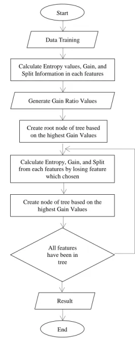
The flowchart of the C4.5 algorithm is as shown in Figure 1.
Figure 1: Flowchart ofC4.5 algorithm
One of the algorithms in decision tree is the C4.5. Tree Start
Data Training
Calculate Entropy values, Gain, and Split Information in each features
Generate Gain Ratio Values
Create root node of tree based on the highest Gain Values
Calculate Entropy, Gain, and Split from each features by losing feature
which chosen
Create node of tree based on the highest Gain Values
All features have been in
tree
Result
collection is done by taking the value of each feature [22]. C4.5 algorithm makes a decision tree from top to bottom, where the top attribute is the root, and the bottom is the leaf. One of the advantages of this method is that its effectiveness in analyzing a large number of attributes from existing data and ease of understanding by users [23]. C4.5 algorithm instead of ID3 uses a modification of acquisition information known as the gain ratio [19]. In the C4.5 algorithm, the highest gain ratio value of all features is selected as the root in decision tree [22]. Generally, there are three types of nodes in the decision tree, namely (1) decision node, represented by a box, (2) node of opportunity, represented in the form of a circle, and (3) end node represented in the form of a triangle [24].
In general, the steps involves in building the C4.5 algorithm decision tree are selecting attributes as roots, making branches for each value, dividing the cases in branches, and repeating the process for each branch until all cases in the branch have the same classes.
III. METHODOLOGY
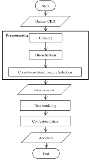
The proposed method of this study started from data processing stage, which includes cleaning, discretization, and correlation-based feature selection (CFS). C4.5 algorithm was used for classification in the data mining process. The purpose of the evaluation stage is to calculate the level of accuracy using the confusion matrix. The stages of the research method are shown in Figure 2.
Figure 2: Stage of the research method
A work step in this study begins with an input of a chronic kidney disease dataset, which is followed by the data preprocessing stage. There are three techniques involved in the data preprocessing. The first technique is the data cleaning process. The purpose of data cleaning is to eliminate missing value in chronic kidney disease dataset. The second technique is the discretization process. Discretization is used to handle continuous value into discrete value. The third technique is the feature selection process using CFS method. CFS method generates values for each feature. Based on these values, the best features can be chosen for the classification process.
The second stage is the data modeling process, which is performed on selected features using C4.5 algorithm. After that, testing process of classification model with testing data is conducted. The evaluation of classification model is based on the testing for predicting the true and false objects using confusion matrix. Confusion matrix evaluation produces an accuracy value, which is the percentage of all data classified correctly. The flow chart of the research method can be seen in Figure 3.
Figure 3: Flowchart of C4.5 algorithm with discretizationand CFS A. Data Processing
Dataset used to diagnose chronic kidney disease was obtained from the UCI machine learning repository uploaded in 2015. This data has been collected by Apollo Hospital, India and it has 25 attributes, 11 of which are numeric and 14 nominal types. The attributes that will be used in this study are presented in Table 1.
400 samples from the dataset have been used in the classification algorithm. Among them 250 labels are classified as CKD and 150 labels as not CKD. Before integrating the collected instances with classification techniques, it is very important to prepare a complete data. At first, it can contain problems such as noise that is representations of attribute values that are not identified or missing value. More than 50% of CKD dataset has a missing value. To eliminate the missing value, dataset needs to be cleaned. The median was used as a technique to clean the data. Specifically, each instance in the numeric attribute with a missing value is replaced with a middle value.
In various classifications, discretization method has been carried out before the classification process. In the discretization process, determining the cut point is the most important problem to achieve a better and more efficient classification accuracy for each machine learning algorithm. Cut points can be defined as the real values within a range of continuous values that divide the range into two intervals [10].
The discretization process involves the following steps: a. Sort a continuous attribute values from features that
will be discretized; Data Processing Data Mining Process Evaluation Data Preprocessing Cleaning Discretization CFS Classification C4.5 Algorithm Accuracy Confusion Matrix Preprocessing Start DatasetCKD Fitur selected Discretization
Correlation-Based Feature Selection
Data modeling
Confusion matrix
Accuracy
End Cleaning
b. Evaluate cut points as separations or intervals that are close together for possibility of combination;
c. Divide or combine continuously the value intervals based on criteria until it stops at several points based on criteria.
Table 1
Description for attributes of CKD dataset No
. Attributes Description Type
1 Al Albumin Nominal
2 Ane Anemia Nominal
3 appet Appetite Nominal
4 Ba Bacteria Nominal
5 Cad Coronary disease artery Nominal 6 Dm diabetes mellitus Nominal 7 Htn Hypertension Nominal
8 Pc pus cell Nominal
9 Pcc pus cell clumps Nominal
10 Pe pedal edema Nominal
11 Rbc red blood cells Nominal 12 Sg specific gravity Nominal
13 Su Sugar Nominal
14 Age Age Numeric
15 Bgr blood glucoses Numeric 16 Bp blood pressure Numeric
17 Bu blood urea Numeric
18 Hemo Haemoglobin Numeric
19 Pcv packed cell
volume Numeric
20 Pot Potassium Numeric
21 Rc red blood cell
count Numeric
22 Sc serum creatinine Numeric
23 Sod Sodium Numeric
24 Wbcc white blood cell Numeric
25 Class Class Nominal
CFS evaluates the value of attributes by considering the individual predictive capabilities of each feature. It also evaluates the redundancy between features. Correlation coefficients are used to estimate correlations between subsets of attributes and classes, and correlations between features [21]. The correlation between each feature and class and between two features can be measured. The best attributes are attributes that have a maximum correlation with the class and have minimum correlation with other attributes [19]. In this case, CFS works to match the evaluation with the right size of correlation. CFS can filter irrelevant data, redundant features, and identifies relevant features as long as they do not depend too much on other features quickly [11].
CFS produces subsets with various feature combinations, and each part is evaluated by Pearson correlation in equation (1):
𝑀𝑠=
𝑘𝑟𝑐𝑓
√𝑘 + 𝑘(𝑘 − 1)𝑟𝑓𝑓
(1)
where: M = Correlation between feature subsets s k = Total number of feature
rcf = Average correlation between feature and class
rff = Mean of intercorrelation between feature
A good feature produces low value for rff and produces high
value for rcf., in which both cases lead to minimization of both
values. Finally, the feature subset with the highest value is selected as the best feature [19].
CFS can be calculated using equation (2) as follows.
𝐶𝐹𝑆 = 𝑀𝑎𝑥𝑠 = [ 𝑟𝑐𝑓1+ 𝑟𝑐𝑓2+ ⋯ + 𝑟𝑐𝑓𝑘 √𝑘 + 2(𝑟𝑓1𝑓2+ … + 𝑟𝑓𝑖𝑓𝑗+ ⋯ + 𝑟𝑓𝑘𝑓1)] (2)
where: rcfi= Correlation rfifj= Correlations r = Defined in equation (3) r = ∑ ( 𝑛 𝑖 𝑥𝑖− 𝑥̅)(𝑦𝑖− 𝑦̅) √∑𝑛 ( 𝑖=1 𝑥𝑖− 𝑥̅)2√∑𝑛𝑖=1(𝑦𝑖− 𝑦̅)2 (3)
where: n = Sample size
xi, yi= Individual samples with the i index
There are several steps that must be done for making a decision tree in the C4.5 algorithm [22]:
a. Prepare training data. Training data obtained from historical data that has happened before. Training data called past data and has been grouped into certain classes.
b. Count the roots of a tree. Entropy is used to select the optimal value that divides the node. Optimal value is considered as important information. Meanwhile, node with high entropy values will be reduced. To calculate the entropy value, equation (4) is used:
𝐸𝑛𝑡𝑟𝑜𝑝𝑦 (𝑆) = ∑ −𝑝𝑖 𝑙𝑜𝑔2(𝑝𝑖) 𝑛
𝑖=1
(4) where: S = Set of cases i
n = Partition S pi = Proportion Si to S
c. Next, calculate the gain value using the entropy result with equation (5). 𝐺𝑎𝑖𝑛(𝑆, 𝐴) = 𝑒𝑛𝑡𝑟𝑜𝑝𝑦 (𝑆) − ∑|𝑆𝑖| |𝑆|Entropy(𝑆𝑖) 𝑛 𝑖=1 (5)
where: S = Set of cases A = Feature
n = Partition of attributes |Si| = Proporsion Sito S
|S| = Cases in S
d. Then, calculate root of a tree. Root of tree are obtained from the attributes to be selected, by calculating the value of gain ratio of each attribute. The highest value of gain ratio becomes the first root. Gain ratio is calculated based on split information, which is calculated using equation (6).
𝑆𝑝𝑙𝑖𝑡𝐼𝑛𝑓𝑜𝑟𝑚𝑎𝑡𝑖𝑜𝑛 (𝑆, 𝐴) = ∑ − |𝑆𝑖| |𝑆|𝑙𝑜𝑔2 𝑛 𝑖=1 |𝑆𝑖| |𝑆| (6)
where: S = Set of data samples
Si to Sc = Subset of data samples that are divided
based on the number of variation values in attribute A.
Next, the gain ratio is formulated as Information Gain divided by Split Information in equation (7).
𝐺𝑎𝑖𝑛𝑅𝑎𝑡𝑖𝑜(𝑆, 𝐴) = Gain(S, A)
𝑆𝑝𝑙𝑖𝑡𝐼𝑛𝑓𝑜𝑟𝑚𝑎𝑡𝑖𝑜𝑛(𝑆, 𝐴) (7)
e. Repeat step 2 to all partitioned records.
f. Decision tree partitioning will stop when all records in node n get the same class. There is no attribute in the partitioned record and no record in the empty branch. B. Evaluation
Evaluation technique is used to test the ability of the classifier that has been built. The evaluation technique adopted in this study was the 10-fold cross validation, which partitioned the D data set randomly into mutually independent 10-fold: f1, f2, .., f10, so that each fold contains
1/10 data section. Then, the 10form of the data set: D1, D2,..., D10 , in which each contains (10-1) fold for tert data, 1 fold for
training data. In the 10-fold cross validation method, classifier accuracy can be calculated by the total number of correctly predicted by classifier divided by all tuples in the data set [25].
In an experiment using the WEKA tool, accuracy is calculated using confusion matrix. Confusion matrix is calculated by comparing the number of correct predictions and the number of false predictions. The evaluation with confusion matrix is shown in Table 2.
Table 2
Evaluation with Confusion Matrix
Actual Class Predicted Class Positive Negative
Positive TP FN
Negative FP TN
Accuracy is obtained from equation (8).
𝐴𝑐𝑐𝑢𝑟𝑎𝑐𝑦 = 𝑇𝑃 + 𝑇𝑁
𝑇𝑃 + 𝐹𝑃 + 𝑇𝑁 + 𝐹𝑁 𝑥 100% (8)
where: TP (True Positive) = Number of positive actual class correctly predicted
TN (True Negative) = Number of negative actual class correctly predicted
FP (False Positive) = Number of negative actual class that are incorrectly predicted
FN (False Negative) = Number of positive tuples that are incorrectly predicted.
IV. RESULT AND DISCUSSION
In this study, the method was tested using WEKA tool. The data used was the CKD dataset obtained from the UCI machine learning repository. This dataset consists of 400 instances, which are divided into 1 class attribute and 24 attributes. Class attributes were used to diagnose the presence or absence of chronic kidney disease in a person.
Before doing the classification using the proposed algorithm, data must be prepared in advance with the aim of minimizing errors and optimizing the results of the classifier. This process is called data pre-processing stage. In this study, three stages of pre-processing data were carried out.
A. Data Cleaning
Data cleaning is done to clear missing value. There were many missing values in the CKD dataset, which are more than 50%. Therefore, this missing value cannot be ignored. In this study, the missing value was cleaned using the median or value of the set of n data in a numeric attribute. To calculate the median of the set n, firstly, the data was sorted. For n odd, the median is the value that is in the middle of the ordered set of values. As for n even numbers, the median was calculated from the average of two values in the middle of the set that has been sorted.
Data cleaning for nominal attributes was done by using the most frequent. After the data with nominal attributes is cleared, the data must be transformed into numerical data so that it can be used in the next process.
B. Discretization Process
Discretization is done to handle attributes that are continuous. Discretization serves to filter instances by discretizing numeric attributes in the dataset so that the instance in the attribute becomes more regular.
The discretization process is as follows:
a. Sort the continuous attribute values of features that will be discretized. By default, discretization will discretize all attributes (first-last).
b. Evaluate cut points as separations or intervals that are close together for possible combination.
c. Divide or combine value intervals based on criteria continuously until it stops at several points based on criteria.
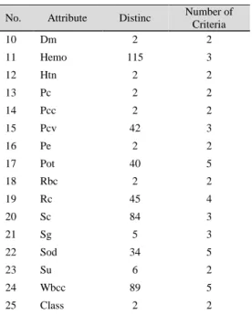
The result of the discretization process is a discrete value attribute. Discretization converts attributes with diverse or distinct data into a number of criteria. Results of the discretization process can be seen in Table 3.
Table 3
Result of the Dicretization Process
No. Attribute Distinc Number of Criteria 1 Age 76 3 2 Al 6 2 3 Ane 2 2 4 appet 2 2 5 Ba 2 2 6 Bgr 146 2 7 Bp 10 2 8 Bu 118 2 9 Cad 2 2
No. Attribute Distinc Number of Criteria 10 Dm 2 2 11 Hemo 115 3 12 Htn 2 2 13 Pc 2 2 14 Pcc 2 2 15 Pcv 42 3 16 Pe 2 2 17 Pot 40 5 18 Rbc 2 2 19 Rc 45 4 20 Sc 84 3 21 Sg 5 3 22 Sod 34 5 23 Su 6 2 24 Wbcc 89 5 25 Class 2 2
Table 4 shows an example of blood pressure (bp) attribute that has data with 10 different types, after the discretization attribute is divided into 2 groups or labels, namely labels <85 and >85.
Table 4
The Result of Discretization Process for bp Attribute
No. Label Count
1 < 85 316
2 > 85 84
C. Correlation-based Feature Selection (CFS)
CFS is done to eliminate redundant or irrelevant features. CFS works by evaluating value of attribute subset. This method of evaluation considers the ability of individual predictions with each feature. CFS can be calculated using the Pearson's correlation coefficient equation. The equation evaluates correlation results of each feature or attribute. Only attribute with the best value will be selected. The best attributes are attributes that have a high correlation with the class label, but have a low correlation with other features. List of selected attributes by applying CFS can be seen in Table 5.
Table 5 Selected Features No Attribute Description 1 Al Albumin 2 Appet Appetite 3 Bp blood pressure 4 Brg blood glucoses 5 Dm diabetes mellitus 6 Hemo Haemoglobin 7 Htn Hypertension 8 Pcv packed cell volume
9 Pe pedal edema
10 Pot Potassium
11 Rc Red blood cell count 12 Sc serum creatinine 13 sg specific gravity
14 Sod Sodium
15 Class Class
Using the CFS method, the process of feature selection produced 14 attributes and 1 class attribute. This attribute will be used in the classification process.
The next step is data modeling. Classification model is made by C4.5 algorithm. The followings are the stages in the C4.5 algorithm:
a. Prepare training data. The distribution of training data and data testing was done using 10-fold cross validation.
b. Calculate entropy value with equation (4). Entropy was used to measure homogeneity or diversity in CKD dataset, where entropy value was calculated from 400 instances in 2 classes (CKD and notCKD).
c. Calculate gain value by reducing entropy value with entropy value of each attribute using equation (5). Information gain was defined as a measure of effectiveness of an attribute in classifying data. The attributes used are attributes that have been selected using CFS.
d. Look for the value of split information from 14 attributes using equation (6).
e. Look for the value of gain ratio. Gain ratio was formulated as Information Gain divided by Split Information. The highest value of gain ratio will be used as a node in decision tree.
f. Repeat step 2 to all partitioned records.
g. Decision tree partitioning will stop when all records in node n get the same class. There are no attributes in partitioned record. And no records in the empty branch. The result of the evaluation was in the form of a list with performance statistics that show the accuracy of the model classifier in predicting the actual class to test option. For option 10-fold cross validation, there are 400 instances tested in 10 iterations. The results showed that there are 389 instances (97.25%) with correct prediction and 11 instances (2.75%) with incorrect predictions. The evaluation results of the C4.5 algorithm with discretization can be seen in Table 6.
Table 6
Evaluation Result of C4.5 Algorithm with Discretization Classified Instances Value (in %) Correct prediction 389 97.25 Incorrect prediction 11 2.75 total number of instances 400
The evaluation result with confusion matrix showed how many instances are predicted in each class and the number of instances that match the actual label. Confusion matrix from C4.5 algorithm with discretization showed the results from the 400 data: i) 6 data were predicted wrongly and 244 data were predicted correctly from the 250 data classified as CKD; ii) 5 data were predicted wrongly and 145 were predicted correctly from the 150 data classified as notCKD. The evaluation result of the confusion matrix of C4.5 algorithm with discretization can be seen in Table 7.
Table 7
Evaluation Result with Confussion Matrix of C4.5 Algorithm with Discretization
Classified CKD notCKD
ckd 244 6
notckd 5 145
The result of the accuracy of the correct classification was obtained:
𝐴𝑐𝑐𝑢𝑟𝑎𝑐𝑦 =244 + 145
400 𝑥 100% = 97.25%
The evaluation results from C4.5 algorithm by applying discretization and CFS showed 390 instances (97.5%) of correct class predicted, and 10 instances (2.5%) incorrect predictions. The evaluation result of C4.5 algorithm with discretization and CFS can be seen in Table 8.
Table 8
Evaluation Result of C4.5 Algorithm with Discretization and CFS Classified Instances Value (in %)
correctly 390 97.5
incorrectly 10 2.5
total number of instances 400
The evaluation result with the confusion matrix shows how many instances are predicted for each class and number of instances that match actual label. C4.5 algorithm's confusion matrix with discretization and CFS showed that out of the 400 data, 5 data were predicted wrongly and 245 data were predicted correctly from the 250 data classified as CKD. 5 data were predicted wrongly and 145 were predicted correctly from the 150 data classified as notCKD. The evaluation result of the confusion matrix from C4.5 algorithm with discretization and CFS can be seen in Table 9.
Table 9
Evaluation Result of C4.5 Algorithm with Discretization and CFS
Classified CKD notCKD
ckd 245 5
notckd 5 145
The result of the accuracy of the correct classification was:
𝐴𝑐𝑐𝑢𝑟𝑎𝑐𝑦 =245 + 145
400 𝑥 100% = 97.5%
The results that show the comparison of the accuracy ratio that uses C4.5 algorithm method before and after discretization with the addition of CFS methods is presented in Table 10.
Table 10
Accuracy Comparison of C4.5 Algorithm
Algorithm Accuracy
C4.5 algorithm 97.00 %
C4.5 algorithm using discretization 97.25 % C4.5 algorithm using discretization
and CFS 97.50 %
V. CONCLUSION
In data mining, data pre-processing is very important because it helps to increase data quality and produces higher accuracy. In this study, data preprocessing was carried out by using discretization and correlation-based feature selection methods. Discretization was used to handle data that is continuous, while correlation-based feature selection was used as attribute selection. Experiment was conducted with WEKA tool. By applying discretization and correlation-based feature selection in the C4.5 algorithm, it was found that there was an increased in the accuracy of 0.5%. Algorithm C4.5 has the accuracy of 97%, while the accuracy result of C4.5 algorithm with discretization was 97.25% and the accuracy obtained from C4.5 algorithm with discretization and correlation-based feature selection was 97.5%. Therefore, it can be concluded that the accuracy of C4.5 algorithm can be increased by applying discretization and correlation-based feature selection for chronic kidney disease diagnosis.
ACKNOWLEDGMENT
Thanks to Mr. Much Aziz Muslim, S. Kom., M. Kom., As our final task supervisor who accompanied us in the process of making this article.
REFERENCES
[1] M. H. A. Elhebir, A. Abraham, “A Novel Ensemble Approach to Enhance the Performance of Web Server Logs Classification”,
International Journal of Computer Information Systems and Industrial Management Applications, vol. 7, 2015, pp. 189-195.
[2] M. A. Muslim, S. H. Rukmana, E. Sugiharti, and B. Prasetiyo, “Application of the pessimistic pruning to increase the accuracy of C4.5 algorithm in diagnosing chronic kidney disease”, Journal of Physics: Conference Series, 2018.
[3] I. H. Witten, E. Frank, Practical Machine Learning Tools and Techniques, USA: Elsevier, USA, 2016.
[4] G. Kaur, E. A. Sharma, “Predict Chronic Kidney Disease Using Data Mining Algorithms In Hadoop”, International Journal of Engineering Researches and Management Studies, vol. 5, no. 2, pp. 34–48, 2018. [5] A. Widodo, S. Handoyo, “The Classification Performance Using
Logistic Regression And Support Vector Machine (SVM)”, Journal of
Theoretical and Applied Information Technology, vol. 95, no. 19, pp. 5184-5194, 2017.
[6] P. Sinha, P. sinha, “Comparative Study of Chronic Kidney Disease Prediction using KNN and SVM”, International Journal of Engineering Research & Technology (IJERT), vol. 4, no.12, pp. 608-612, 2015.
[7] M. Zavvar, A. Yavari, S. M. Mirhassannia, M. R. Nehi, and M. H. Zavvar, “Classification of Risk in Software Development Projects using Support Vector Machine”, Journal of Telecommunication, Electronic and Computer Engineering, vol. 9, no. 1, pp. 1-5, 2017. [8] H. F. Eid, A. Abraham, “Adaptive Feature Selection and Classification
Using Modified Whale Optimization”, International Journal of Computer Information System and Industrial Management Applications, vol. 10, 2018, pp. 174-182.
[9] R. Asgarnezhad, M. Shekofteh, and F. Z. Boroujeni, “Improving Diagnosis of Diabetes Mellitus Using Combination of Preprocessing Techniques”, Journal of Theoretical and Applied Information Technology, vol. 95, no. 13, pp. 2889-2895, 2017.
[10] P. Kapoor, D. Arora, and A. Kumar, “Implications of Discretization Towards Improving Classification Accuracy for”, Journal of Theoretical and Applied Information Technology, vol. 95, no. 24, pp. 6893–6901, 2017.
[11] S. Sasikala, “Multi Filtration Feature Selection (MFFS) to improve discriminatory ability in clinical data set”, Applied Computing and Informatics, vol. 12, no. 2, pp. 117–127, 2016.
[12] J. Han, M. Kamber, J. Pei, Data Mining: Concepts and Techniques, CA, itd: Morgan Kaufmann, San Francisco, 2012.
[13] G. I. Salama, M. B. Abdelhalim, and M. A. Zeid, “Experimental comparison of classifiers for breast cancer diagnosis”, 2012 Seventh
International Conference on Computer Engineering & Systems (ICCES), pp. 180-185, 2012.
[14] A. S. Levey, J. Coresh, “Chronic kidney disease”, The Lancet, vol. 379, no. 9811, pp. 165-180, 2012.
[15] M. A. Muslim, I. I. N. Kurniawati, and E. Sugiharti, “Expert System Diagnosis Chronic Kidney Disease Based on Mamdani Fuzzy Inference System”, Journal of Theoretical and Applied Information Technology, vol. 78, no. 1, pp. 70-75, 2015.
[16] Z. A. Altikardes, H. Erdal, A. F. Baba, A. S. Fak, and H. Korkmaz, “Performance evaluation of classification algorithms by excluding the most relevant attributes for dipper/non-dipper pattern estimation in Type-2 DM patients”, International Journal of Computer Information System and Industrial Management Applications, vol. 8. 2016, pp. 247-256.
[17] R. Dash, R.L. Paramguru, R. Dash. “Comparative Analysis of Supervised an Unsupervised Discretization Techniques”, International Journal of Advances in Science and Technology, vol. 2, no. 3, pp. 29-37, 2011.
[18] A. Al-Ibrahim, “Discretization of Continuous Attributes in Supervised Learning Algorithms”, The Research Bulletin of Jordan ACM, vol. 2, no. 4, pp. 1158, 2011.
[19] M. Hall, Correlation-based Feature Selection for Machine Learning, Methodology, 1999.
[20] S. H. Bouazza, K. Auhmani, and A. Zeroual, “Application of the Filter approach and the Clustering algorithm on Cancer datasets”,
International Journal of Computer Information Systems and Industrial Management Applications, vol. 10, no. 2018, pp. 068-086, 2018. [21] A. G. Karegowda, A. S. Manjunath, and M. A. Jayaram, “Comparative
Study of Attribute Selection Using Gain Ratio and Correlation Based Feature Selection”, International Journal of Information Technology and Knowledge Management, vol. 2, no. 2, pp. 271–277, 2010. [22] M. A. Muslim, A. Nurzahputra, and B. Prasetiyo, “Improving Accuracy
of C4.5 Algorithm Using Split Feature Reduction Model and Bagging Ensemble for Credit Card Risk Prediction”, 2018 International Conference on Information and Communication Technology, pp. 141– 145, 2018.
[23] W. Dai, W. Ji, “A MapReduce Implementation of C4.5 Decision Tree Algorithm”, International of Database Theory and Application, vol. 7, no. 1, pp. 49-60, 2018.
[24] A. M. Alfatah, R. Arifudin, and M. A. Muslim, “Implementation of Decision Tree and Dempster Shafer on Expert System for Lung Disease Diagnosis”, Scientific Journal of Informatics, vol. 5, no. 1, pp. 50-57, 2018.
[25] K. R. Lakshmi, Y. Nagesh, and M. Veerakrishna, “Performance Comparison of Three Data Mining Techniques for Predicting Kidney Dialysis Survivability”, International Journal of Advances in Engineering & Technology, vol. 7, no. 1, pp. 242-254, 2014.