THE CENTER FOR THE STUDY
OF
I
NDUSTRIAL
O
RGANIZATION
AT NORTHWESTERN UNIVERSITY
Working Paper #0016
Simple Menus of Contracts in Cost-Based
Procurement and Regulation
By
William P. Rogerson
Department of Economics and Institute for Policy Research, Northwestern University
SIMPLE MENUS OF CONTRACTS
IN COST-BASED PROCUREMENT AND REGULATION ABSTRACT
This paper develops an extremely simple formulation of the Laffont-Tirole principal agent model
of cost-based procurement and regulation which is suitable for applied uses by restricting the
principal to using a two item menu where one item is a cost-reimbursement contract and the other
item is a fixed price contract. Menus of this form are called fixed-price-cost-reimbursement
(FPCR) menus. In the case where the agent’s utility is quadratic and the agent’s type is distributed
uniformly, it is shown that the optimal FPCR menu always captures at least three quarters of the
gain that the optimal complex menu achieves. Therefore, at least for the uniform quadratic case,
extremely simple menus with low informational requirements perform nearly as well as the fully
1. INTRODUCTION
In an influential paper, Laffont and Tirole (1986) formulated a principal agent model of
cost-based procurement and regulation and showed that the principal can implement the optimal
mechanism by offering the agent a menu consisting of a continuum of linear contracts. Two1
related problems with applying this theory in practice have been that the economic logic and the
underlying mathematics involved in calculating the optimal menu are quite complex, and the
principal must be able to specify the agent’s entire disutility of effort function in order to calculate
the optimal menu. As a result, the model has not been widely used in practice to either calculate
actual incentive contracts or even to develop useful qualitative guidance about the nature of the
optimal solution and how it is affected by various economic factors. This paper develops an
extremely simple formulation of the Laffont-Tirole principal agent model which is very amenable
to such applied uses by restricting the principal to using a two item menu where one item is a
cost-reimbursement contract and the other item is a fixed price contract. Menus of this form are
called fixed-price-cost-reimbursement (FPCR) menus.
Under asymmetric information, the normal problem with offering a fixed price contract
(i.e., a menu with a single item which is a fixed price contract) is that the fixed price must be set
equal to a very high value in order to guarantee that even high cost types will be willing to
produce the good. An FPCR menu solves this problem because all types of the agent are willing
to accept the cost reimbursement contract. This frees the principal to choose a much lower fixed
price in order to focus on providing incentives and extracting rent from the low cost types.
Calculation of the optimal FPCR menu is very straightforward and intuitive and the
to calculate the optimal FPCR menu. In the case where the agent’s utility is quadratic and the
agent’s type is distributed uniformly, it is shown that the optimal FPCR menu always captures at
least three quarters of the gain that the optimal complex menu achieves. Therefore, at least for the
uniform quadratic case, extremely simple menus with low informational requirements perform
nearly as well as the fully optimal complex menu.
The paper also considers a more general notion of simple menus where the fixed price
contract is replaced by a linear contract. (i.e., the principle offers the agent a choice between a
linear contract and a cost reimbursement contract.) In the linear quadratic case, the optimal
simple menu of this more general sort always achieves at least 8/9 of the gains achieved by the
optimal complex menu.
This paper calculates a closed form solution for the principal’s expected procurement cost
under the fully optimal menu for the uniform quadratic case in order to compare the performance
of simple menus to that of the fully optimal complex menu. However, given that these
calculations are presented, it is possible to make an additional observation that may be of some
independent interest. Namely, plausible ranges of parameters exist where the principal’s expected
procurement costs are significantly increased by the presence of asymmetric information, but
where the principal gains very little from using the fully optimal mechanism instead of simply
using a cost reimbursement contract. That is, plausible ranges of parameters exist where
asymmetric information is a serious problem for the principal but incentive contracting is of very
little value to the principal is dealing with this problem. Of course this result should not
necessarily be viewed as surprising, since nothing in the abstract theory of incentives suggests
This paper’s research was originally motivated by a policy issue in defense procurement.
In the United States, the Department of Defense (DOD) purchases almost all major weapons
systems from sole source contractors using contracting methods that essentially amount to using
cost reimbursement contracts. The best way to understand why DOD uses cost reimbursement2
contracting methods is that they perform precisely the function identified in Laffont and Tirole’s
principal agent model; they guarantee, in a situation that amounts to a bilateral monopoly, that
DOD and the firm can reach an agreement (i.e., they guarantee that the agent will always produce
the good.) Of course the use of cost reimbursement contracting methods creates very poor
incentives for cost reduction. The idea motivating this paper’s research was that a simple way to
improve incentives but still retain the desirable property that agreement was always reached
would be to allow the contracting officer to make a fixed price offer to the contractor prior to the
beginning of the normal contracting process. If the contractor accepted this price, then
production would occur under a fixed price contract at that price. However, if the contractor
rejected the price, then normal contracting procedures would continue. That is, the contracting
officer could allow the contractor the opportunity to opt out of the normal cost reimbursement
contracting process but still be able to fall back on this process if necessary.
In theory, the contracting officer would do best by offering a menu with a continuum of
choices, as calculated by Laffont and Tirole, as an alternative to cost reimbursement contracting.
In practice it is hard to imagine that the contracting officer would have either the detailed
information about the agent’s disutility function or the computational ability to attempt to offer
such a complex menu. A much more modest goal would be to hope that the contracting officer
procedures were followed and to suggest what the size of the efficiencies from fixed price
contracting would be. This is enough to calculate the optimal simple fixed price menu. In fact, it
turns out that when the distribution of costs is uniform, the contracting officer does not even need
to know the precise size of efficiencies that would result from fixed price contracting in order to
calculate the optimal fixed price.
The model can also be interpreted as capturing the situation where a regulator offers a
utility a price cap with the option that the normal regulatory process will continue if the firm
declines to accept the price cap. This is arguably the type of negotiation that actually has been
occurring between regulators and utilities.
There are three papers in the literature ( Reichelstein 1992, Bower 1993, Gasmi, Laffont
and Sharkey 1999) that evaluate the performance of simple mechanisms in Laffont-Tirole type
principal agent models. These papers have already provided examples where certain types of
simple mechanisms can perform well and performed calculations with the uniform quadratic
model. However, none of these papers consider the general idea of using a two item menu where
one item is a cost reimbursement contract (to guarantee that all types accept a contract) and one
item is a simple incentive contract (to provide incentives and extract rent from at least some
types.) In particular, none of these papers consider the idea of an FPCR menu. Furthermore,
none of these papers identify any other type of simple mechanism that “always” works nearly as
well as the fully optimal mechanism over a complete range of parameter values.
Gasmi, Laffont and Sharkey(1999) ( GLS) present calculations of the welfare gain from
using various regulatory mechanisms in a principal agent model of telecommunications regulation.
functional forms are too complicated to allow general closed form solutions. Instead, GLS use a
calibration process to choose plausible values for the parameters and then use the computer to
numerically evaluate the performance of various types of regulatory mechanisms given the chosen
parameter values. For the parameter values they choose, they conclude that price cap regulation
performs nearly as well as the fully optimal mechanism and that both of these mechanisms perform
significantly better than simple cost based regulation. The regime of price cap regulation in GLS
corresponds to a regime where the principal offers a single fixed price contract in this paper’s
model. In the GLS model, the analog of an FPCR menu would be an “optional price cap plan”
where the firm was offered the choice between accepting a price cap or remaining under
traditional cost based regulation. GLS do not consider such an optional price cap plan. Of course,
given the parameters they choose, there is little need to consider an optional price cap plan,
because even the (non-optional) price cap plan works nearly as well as the fully optimal
mechanism. The results of this paper suggest that plausible parameter values could be chosen in
the GLS model where a (non-optional) price cap plan would not perform well, but that an
optional price cap plan might continue to perform nearly as well as the fully optimal mechanism. 3
Reichelstein(1992) describes a situation in Germany where the German Department of
Defense offered a contractor a menu of linear contracts for a particular procurement. Reichelstein
advised them on how the menu should be constructed based his analysis of the Laffont Tirole
model. The menu actually used had seven alternatives in it and Reichelstein calculated the optimal
menu assuming quadratic disutility and allowing for a variety of different distributional functions.
Therefore he presented the German DOD with a situation where, if they were willing to specify
seven item menu would be automatically calculated. However, the whole formulation was
apparently complex enough that the German DOD did not use it to actually calculate the menu it
used. Rather, it simply chose cost shares in a fairly arbitrary way so that they varied fairly
smoothly over the range of target costs specified. This experience nicely illustrates the point that
theoretically superior mechanisms may not prove to be superior in practice if their calculation
and/or information requirements overwhelm the capabilities of the principal.
Bower (1993) considers a more complex model than the basic Laffont-Tirole model, so
the connection between Bower’s model and this paper’s model is not as close. The Bower model
is dynamic and allows for interim auditing. In this model, he compares the benefit from using a
complex menu of linear contracts in the last period of the model to a single linear contract in the
last period of the model when disutility is quadratic and the distribution of costs is uniform. He
finds, given the parameter values he investigates, that a single linear contract (i.e., a menu
consisting of a single choice which is a linear contract) performs almost as well as the menu.
However, Bower implicitly restricts himself to parameter values where the asymmetric
information problem is small relative to the moral hazard problem. When the amount of
asymmetric information grows larger, a single linear contract performs much more poorly than the
fully optimal menu. The contribution of this paper relative to Bower is show that, even when the
amount of asymmetric information is large so that a menu with a single linear contract does not
perform well, a menu with a linear contract plus a cost reimbursement contract can continue to
perform very well.
In a research project whose results are reported in a book, Wilson(1993) conducts a
towards providing guidance for employing non-linear pricing schemes in practice. Wilson’s
results are not as closely related to those of this paper or to those of the other papers described
above because the structure of the non-linear pricing model is somewhat different than the
structure of the procurement/regulation model. However, Wilson proves a “speed of
convergence” result that has a similar flavor to the result of this paper. Namely, Wilson identifies
circumstances such that, as the number of menu items the principal is allowed to use increases, the
performance of the optimal menu converges “rapidly” to the performance of the fully optimal
menu.
The paper is organized as follows. Section 2 presents the basic model. Section 3 solves
for the optimal FPCR menu and Section 4 compares the performance of the optimal FPCR menu
to the optimal complex menu for the uniform quadratic case. Section 5 makes some observations
about the value of incentive contracting in the uniform quadratic case. Section 6 considers a
more general type of simple menu where the fixed price contract is replaced by a linear contract.
Finally Section 7 draws a brief conclusion.
2. THE MODEL
A risk-neutral principal wishes to purchase one unit of a good from an agent. Before the
game begins, nature chooses a parameter x, called the agent’s type, according to the distribution4
F(x) with density function f(x) defined over some non-negative interval [x , xmin max]. The agent
observes the value of x but the principal only knows the distribution from which x is drawn . Let
(2.1) H(x) = F(x)/f(x).
Assume that
(a.1) f(x) is strictly positive and H(x) is strictly increasing over the interval [x , xmin max].
Let y [0, ) denote the amount of cost reduction achieved by the agent through exerting effort to reduce costs and let 1(y) denote the dollar value of disutility that the agent experiences if costs are reduced by y. The actual cost of production, c, is given by
(2.2) c = x - y.
Assume that the principal can directly observe and measure the actual cost of production, c, but is
unable to directly observe or measure either y or 1(y). Let s(y) denote the social surplus created if the agent chooses a level of cost reduction equal to y.
(2.3) s(y) = y - 1(y).
The level of cost reduction that maximizes social surplus will be called the first best level of cost
reduction. Assume that
the first best level of cost reduction is positive.
Let y denote the first-best level of cost reduction and let k denote the resulting surplus.F
(2.4) k = y - s(y ).F F
Since the principal is able to directly observe and measure c, the principal is able to enter
into contracts with the agent that specify the price the principal will pay the agent as a function of
what production costs actually turn out to be. The game unfolds as follows. First, the principal5
offers the agent a menu of contracts specifying price as a function of c. Then the agent decides
which contract, if any, to accept. If the agent does not accept any contract, the game is over,
production does not occur, the agent exerts no effort, and the principal makes no payment to the
agent. If the agent does accept a contract, then production occurs, the cost of production is
realized and the principal pays the agent the price specified by the contract that was accepted.
The principal’s problem is to offer the agent a menu of contracts that minimizes his expected
payment to the agent, subject to the constraint that all types of the agent accept a contract and
produce the good.
A theoretical lower bound on the principal’s expected procurement cost is the
procurement cost that he could achieve if he had full information, i.e., if he could directly observe
x and y. In this case the principal would minimize his procurement cost by offering to pay an
agent of type x a fixed price equal to x - k. (The agent would accept this contract, choose the
procurement cost would be m - k, where m denotes the expected value of x.
A very simple way for the principal to guarantee that he always procures the good would
be to offer the agent a cost reimbursement contract. Under a cost reimbursement contract, the
principal promises to pay the agent a price equal to the measured cost of production, c. Under
such a contract, every type would engage in no cost reduction and earn zero profit, so would be
(weakly)willing to accept such a contract. An agent of type x would produce at a cost of x and
receive a payment of x from the principal. Therefore the principal’s expected payment when he
uses a cost reimbursement contract is m. This means that the principal loses k dollars relative to
the first best by using a cost reimbursement contract. Subsequent sections will investigate the
extent to which progressively more complicated mechanisms can reduce this loss.
3. FPCR MENUS
In this section, the principal will be allowed to offer the agent a menu of two contracts,
one of which is a cost reimbursement contract and the other of which is a fixed price contract.
This will be called a fixed-price-cost-reimbursement (FPCR) menu. The only variable of choice
for the principal is the fixed price of the fixed price contract. Part A will consider the general case
and parts B will apply this result to the case where the distribution of types is uniform. Part C
describes an interesting property of the optimal FPCR menu that holds for the general case.
A. The General Case
Suppose the principal offers the agent an FPCR menu with fixed price p. It is
straightforward to see that all types less than or equal to p + k will accept the fixed price
Lemma 3.1:
If the principal offers an FPCR menu with fixed price p, all types of the agent less than or equal to
p + k will accept the fixed price contract.
Proof:
Consider an agent of type x. If the agent declines to accept the fixed price contract, he will
operate under the cost reimbursement contract and earn zero profit. If the agent accepts the fixed
price contract, and chooses a level of cost reduction equal to y, his profit will be given by
(3.1) p - x + y - 1(y).
Under a fixed price contract the agent will therefore maximize his profit by choosing the first best
level of cost reduction, y , in which case his utility will be given by F
(3.2) p - x + k .
Expression (3.2) is non-negative if and only if the agent’s type is less than or equal to p+ k. QED
The highest type willing to accept the fixed price will be called the cut-off type and be
denoted by . Note that an FPCR menu can be described equally well by specifying the value of the fixed price it offers, p, or the value of the cut-off type it induces, . The FPCR menu
inducing the cut-off type is the same as the FPCR menu with the fixed price -k. Both methods of referring to FPCR menus will be used interchangeably in this paper.
(3.3) C() P x xxmin ( k)f(x) dx P xxmax x x f(x) dx An FPCR menu will be defined to be optimal if it minimizes the principal’s expected
procurement costs over the set of all FPCR menus. It is clear that all FPCR menus with price less
than or equal to x - k generate the same expected procurement cost for the principal, and thatmin 7
all FPCR menus with price strictly greater than xmax - k generate strictly higher procurement costs
than the FPCR menu with price equal to xmax - k. Therefore, without loss of generality, the8
search for an optimal FPCR menu can be restricted to menus with fixed prices in the interval [xmin
- k, xmax - k], or, equivalently, to menus that induce cut-off types in the interval [x , xmin max].
In order to characterize the optimal FPCR menu, it will turn out to be convenient to refer
to FPCR menus in terms of the cut-off types they induce. Let C( ) denote the principal’s expected procurement cost if he chooses the FPCR menu that induces the cut-off type . For values of in [x , x ], C() is given bymin max
If the agent’s type is less than , he accepts the fixed price contract and the principal pays a price of - k. If the agent’s type is greater than , he accepts the cost reimbursement contract and the principal pays a price equal to the agent’s type.
The derivative of this function is given by
The form of this derivative is very intuitive. Raising by one dollar has two effects on procurement costs. The first effect is that all types of the agent below (who are already accepting the fixed price contract) will be paid one more dollar. There are F() of these types. Therefore procurement cost will go up by F(), which is the first term of (3.4). The second effect of raising is that some types will switch from the cost reimbursement contract to the fixed price contract. For the cutoff type, the principal’s gain from this switch is equal to k. The9
number of such types is equal to f(). Therefore procurement cost will go down by kf(), which is the second term of (3.4).
Substitution of (2.1) into (3.4) yields
(3.5) C1() = f() { H()-k}.
Therefore the sign of C1() is determined by the sign of the bracketed term in (3.5). Assumptions (a.1)- (a.2) guarantee that H(0) = 0, H(x) is strictly increasing, and k is strictly positive. This
immediately implies that there is a unique value of that minimizes C() over the interval [x , xmin max] . If there is a value of such that H() is equal to k, then this is the optimal cut-off type. If H() remains below k for every [x , x ], then the optimal cut-off type is x min max max. Proposition 3.1 formally states the result.
Proposition 3.1:
There is a unique FPCR menu that minimizes the principal’s expected procurement costs over the
H (k) if -1 H(xmax) k (3.6) * =
xmax if H(xmax) < k
The fixed price offered under the optimal FPCR menu is given by
(3.7) p * = F * - k
Proof:
As above. QED
In summary, there is a very clear, simple, and intuitive solution to the problem of choosing
the optimal FPCR menu. In order to use this in real contracting situations a principle would need
to be able to describe the likely distribution of costs if a cost-reimbursement contract was used
(this is F(x)) and the size of the efficiency that he believes would be induced by fixed price
contracting (this is k). Given these two pieces of data, calculation of the optimal FPCR menu is
straightforward. Furthermore, the requirement that the hazard rate in strictly increasing would
not actually be needed to use this rule in practice. This assumption simplified the exposition
because it guaranteed that there was a unique local maximum (which was, therefore, the global
maximum). In practice, the principle could specify any distribution and use a computer to directly
calculate C() over the entire range of values for . Therefore distributions that allowed multiple local optima would not pose any major problem.
This part will analyze the case where the density of types is uniformly distributed over
[x , xmin max]. As above, let k denote the first best efficiency gain. Let denote the spread between the highest cost and lowest cost types.
(3.8) = x - xmax min
Proposition 3.2 now describes the particularly simple form the optimal FPCR menu takes
for this case. Namely, the fixed price is equal to the minimum of x and xmin max - k.
Proposition 3.2:
Suppose that the agent’s type is uniformly distributed over [xmin, maxx ] and that the level of
efficiencies achievable under the first best is equal to k. Then the fixed price under the optimal
FPCR menu is given by
xmin k
(3.9) p* =
xmax - k, k or equivalently by
(3.10) p* = min {x , xmin max - k}.
Proof:
(3.11) F(x) = (x - x ) / min . (3.12) f(x) = 1 /
(3.13) H(x) = x - x .min
Substitution of (3.13) into (3.6) yields
xmax, if k
(3.14) * =
x +k,min if k.
Substitution of (3.14) into (3.7) yields (3.9). QED
To interpret the result, note that if the principal offers a FPCR menu with a fixed price
equal x , the principal will induce all types less than or equal to x + k to accept the fixed pricemin min
contract. Proposition 3.2 states that it is optimal for the principal to offer a fixed price equal to
x unless even the highest cost type strictly prefers the fixed price contract (i.e., unless xmin min + k >
xmax) . In this case, it is optimal for the principal to lower the fixed price until the highest cost
type is indifferent between the fixed price contract and the cost reimbursement contract (i.e. to
offer a fixed price equal to xmax - k).
Three remarks are worth noting about the solution for the uniform case. First, the
solution for the uniform case is particularly simple. The fixed price under the optimal menu is
simply equal to the minimum of x and xmin max - k. Second, the optimal FPCR menu exhibits what
to never be made worse off in any state of the world by switching from a regime of using cost
reimbursement contracting to a regime of offering the optimal FPCR menu. This is because the
principal never offers a price higher than xmin min as part of the optimal FPCR menu, and x is, by
definition, the lowest possible amount that the principal would ever pay under cost reimbursement
contracting. In real situations, where a purchasing organization was considering whether or not
to use a simple menu of contracts instead of a cost reimbursement contract, this property might be
viewed as a very desirable feature. Third, there is a sense in which the information requirements
for the uniform case may sometimes be considerably less demanding than the information
requirements for the general case. In general, the principal needs to know the exact value of the
potential efficiency gains, k, to calculate the optimal FPCR menu. However, for the uniform case,
so long as k is less than , the principal offers a fixed price equal to x independent of the precisemin
value of k. Therefore, if the principal happens to be in a situation where he knows that k is less
than , but he does not know the precise value of k, he is still able to calculate the optimal FPCR menu.
Now the question of how well the optimal FPCR menu performs will be investigated.
Recall that k is the first best level of efficiency gain as defined by (2.4). Let m denote the
expected value of x, given by,
(3.15) m = (x + xmin max)/2
Recall that denotes the spread between the highest and lowest type given by (3.8) and define to be the ratio of to k:
(3.16 ) = /k.
It will be convenient to view a principal agent problem as being characterized by a triple
(k, m, ). Intuitively, think of k as the first best level of efficiency gain, m as the expected value of the agent’s type, and as the spread between the highest and lowest type measured in multiples of k. Let P (k, m, S , ) denote the principal’s expected procurement cost when the
principal uses the optimal FPCR menu in the environment (k, m, ). Corollary 3.1 presents the value of this function.
Corollary 3.1:
m - k + ( k/2) 1 (3.17) P (k, m, S ) =
m - (k/2) 1. proof:
Straightforward algebra based on the result of Proposition 3.2. QED
Since the principal’s expected procurement cost if he uses a cost reimbursement contract
is equal to m, the difference between m and P (k, m, S ) can be interpreted as the principal’s
expected gain to using the optimal FPCR menu instead of simply using a cost reimbursement
contract. Let g (k, m, S ) denote this gain, expressed as a fraction of the first best efficiency gain.
(3.18) g (k, m, S ) = {m - P (k, m, )}/kS
1 - (/2) 1 (3.19) g (S ) =
1/(2) 1.
Note that g turns out to only depend on S (and not on k or m).
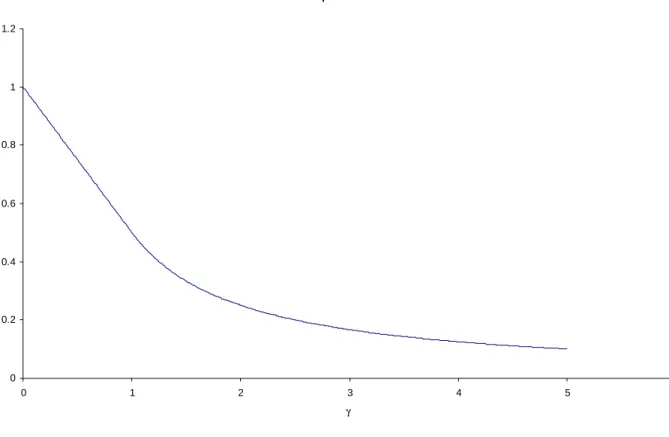
Figure 3.1 presents a graph of g (S ) as varies between 0 and . Note that g is equal toS 1 when is equal to 0, that g decreases as increases, and that g converges to 0 as growsS S
large. This qualitative behavior is very intuitive. The parameter is a measure of the amount of asymmetric information. When is equal to zero there is no asymmetric information and the principal can achieve the first best gain by simply offering the agent a fixed price contract k below
his type. As the amount of asymmetric information grows, the principal’s expected gain
decreases, and in the limit, when there is an infinite amount of asymmetric information, the
principal receives no gain at all from using an FPCR menu instead of using a cost reimbursement
contract.
D. An Upper Bound on the Fixed Price in the Optimal FPCR Menu
Figure 3.1 The Share of the First Best Efficiency Gain Captured by the Optimal FPCR Menu As γ Varies 0 0.2 0.4 0.6 0.8 1 1.2 0 1 2 3 4 5 6 γ
will take a brief digression to show that the result for the uniform case that the fixed price under
the optimal FPCR menu is always less than or equal to x is actually a special case of a moremin
general result. It can be shown that if the density of types is weakly decreasing for every x greater
than or equal to some value x1, then the fixed price under the optimal FPCR menu is always less than or equal to x1. The essential idea is that, when the principal offers a fixed price of p as part of an FPCR menu instead of simply offering a cost reimbursement contract, he makes a loss on
types less than p (he would have paid them less than p under a cost reimbursement contract) and
he makes a gain on the types of the agent between p and p +k. (These types accept the fixed price
contract and the principal would have paid them more under a cost reimbursement contract.)
be profitable to the principal if it sufficiently increases the gain he earns on the second group. It is
straightforward to show that the principal will actually earn lower profits on the second group by
raising p if the density of types is decreasing past p.
Proposition 3.3:
Suppose that f(x) is weakly decreasing for every x greater than or equal to some value of x
denoted by x1. Then the fixed price in the optimal FPCR menu is always less than or equal to x1 Proof:
See Appendix A. QED.
4. Complex Menus
This section will compare the performance of the optimal FPCR menu to the performance
of the optimal complex menu (i.e., the optimal menu with no restrictions as to the number of
menu items or their nature) for the case where the distribution of types is uniform and the agent
has quadratic disutility of effort.10
As in section 3 assume that the agent’s type is distributed uniformly over the interval [x ,min
xmax]. In addition, assume that the agent’s disutility of effort function is given by
(4.1) 1(y) = y /4k2
where k is a parameter chosen from (0, ). It is straightforward to verify that, given the
k. Therefore, just as the previous section, the parameter k can be interpreted as the efficiency
gain under the first best and a principal agent problem can be denoted by a triple (k, m, ). Laffont and Tirole (1986, 1993) characterize the optimal mechanism for a class of cases
that includes the uniform quadratic case. Let P (k, m, C ) denote the principal’s expected
procurement cost under the optimal mechanism for the problem (k, m, ). Proposition 4.1 presents the value of this function.
Proposition 4.1:
m - k [ 1 - /2 + /12],2 2 (4.2) P (k, m, C ) =
m - 2k/3, 2 proof:
See Appendix B. QED
Let g (k, m, C ) denote the principal’s gain from using the optimal complex menu instead of using
a cost reimbursement contract expressed as a share of the first best gain. This is defined by
(4.3) g (k, m, C ) = {m - P (k, m, )}/k.C
Substitution of (4.2) into (4.3) yields
1 - /2 + /12,2 2
(4.4) g (C ) =
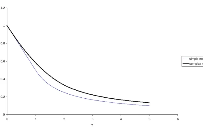
Figure 4.1 The Share of the First Best Efficiency Gain Captured by the Optimal FPCR Menu and the Optimal Complex Menu as γ Varies
0 0.2 0.4 0.6 0.8 1 1.2 0 1 2 3 4 5 6 γ simple menu complex menu
Figure 4.1 presents a graph of g (C ) as varies between 0 and , along with a graph of g (S ) which was calculated in the previous section. Just as for g , the function g is equal to oneS C
when equals 0, is decreasing in , and converges to 0 as grows large. When there is no asymmetric information (i.e., = 0), both the simple and complex menu yield the first best gain of k. However, when there is asymmetric information (i.e, > 0) both types of menu yield a gain strictly less than k and the gain from the optimal simple menu is strictly less than the gain from the
optimal complex menu. Therefore the optimal complex menu does better than the optimal FPCR
menu so long as there is asymmetric information. The question of how much better it does will
Let )() denote the ratio of the gain achieved by the optimal FPCR menu to the gain achieved by the optimal complex menu.
(4.5) )() = g () /g ().S C
Substitution of (3.19) and (4.4) into (4.5) yields
{1 - /2}/{1 - /2 + /12},2 1
(4.6) )() = {1/(2)} / {1 - /2 + /12},2 1 2
3/4, 2
In particular, notice that )() is constant and equal to 3/4 for 2. Visual inspection of Figure 4.1 suggests that the ratio of g to g increases as S C decreases below 2. Straightforward calculus confirms this result.
Therefore, for values of greater than or equal to 2, the optimal FPCR menu captures precisely 75% of the gain that the optimal complex menu can achieve. As decreases below 2, the optimal FPCR menu captures an even larger share of the gains that the optimal complex menu
achieves, and as approaches 0 the optimal FPCR menu captures 100% of the gains achieved by the optimal complex menu.
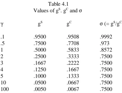
Table 4.1 reports values of g , g , and S C ) for various values of . The values reported in
Table 4.1 are consistent with the observations about the relative performance of the optimal
Table 4.1 Values of g . g and S C ) gS gC ) (= g /g S C) .1 .9500 .9508 .9992 .5 .7500 .7708 .973 1 .5000 .5833 .8572 2 .2500 .3333 .7500 3 .1667 .2222 .7500 4 .1250 .1667 .7500 5 .1000 .1333 .7500 10 .0500 .0667 .7500 100 .0050 .0067 .7500
optimal FPCR menu always produces exactly three quarters of the gain that the optimal complex
menu can achieve. As decreases below 2, the optimal FPCR menu produces an even larger share of the gain achieved by the optimal complex menu.
5. The Value of Incentive Contracting
The main reason that this paper calculated the performance of the optimal complex menu
for the uniform quadratic case was to compare its performance to that of the optimal FPCR menu.
However, given that the performance of the optimal complex menu has been calculated, it is
interesting make another observation about the results of this calculation. Namely, although there
are plausible ranges of parameters for which the optimal mechanism captures a very large share of
the welfare loss due to asymmetric information, there are also plausible ranges of parameters
where even the fully optimal mechanism provides a relatively modest benefit.
Column 3 of table 4.1 displays the share of the welfare loss due to asymmetric information
that the principal is able to recover by using the fully optimal complex mechanism. Performance
a wide range of values of across different procurement and regulation problems, including low values such as = .5 where the optimal mechanism captures a large share of the losses due to asymmetric information and higher values such as = 5 or = 10 where the optimal mechanism captures a very small share of the losses.
For example, suppose that the agent’s type is distributed uniformly over [$80, $120] and
the parameter k is equal to 10. This is relatively plausible example - costs vary plus or minus
twenty percent around the mean and fixed price contracting can yield an efficiency gain of ten
percent. In this example is equal to 4. Reading from the third column of Table 4.1, the optimal complex mechanism captures 16.67 percent of the first best efficiency gain, or $1.67. Therefore,
using the optimal complex menu instead of simply using a cost reimbursement contract reduces
the principal’s expected procurement costs from $100 to $98.33. 11
Three points should be noted about this observation. First, it should not necessarily be
surprising that cases exist where even the optimal mechanism cannot make huge inroads in solving
the problems that asymmetric information creates. Second, if there a small enough incremental
cost to offering a menu of contracts, then the principal will still offer a menu. Third, this example
does suggest, however, that if a principal had to allocate scarce resources between calculating and
implementing optimal incentive contracts and gathering information to reduce asymmetric
information that, at least in some plausible examples, the potential gain to the latter may be larger
than the potential gain to the former. The analysis of this paper suggests that such situations are
likely to occur when the amount of asymmetric information is large relative to the first best
efficiency gain.
A natural question to investigate is whether or not a large share of the gains left
uncaptured by FPCR menus, might be captured by slightly more complex menus that are,
nonetheless, still considerably simpler than the fully optimal menu. A natural candidate to consider
is a two item menu where one item is still a cost-reimbursement contract (which guarantees that
every type of agent will accept a contract) but the other item is allowed to be any linear contract.
A menu consisting of two items where one item is a cost reimbursement contract and one item is a
linear contract will be called a linear-contract-cost-reimbursement (LCCR) menu. Appendix C
presents an analysis of this problem. The main results of this analysis are reported in this section.
Any linear contract can be written in the form
(6.1) p = c + (1- T ) (c - c ) T
where the parameters c and T in (7.1) can be interpreted, respectively, as the target cost and
sharing ratio. According to (7.1), if actual cost turns out to equal the target cost, then the agent
is paid a price equal to the cost. If actual cost rises above (falls below) the target cost by one
dollar, then price rises (falls) by (1- ) dollars, so that the agent bears of the cost overrun (underrun).
The optimal FPCR menu can be viewed as the result of setting equal to 1 and solving for the optimal value of c . (When T is set equal to 1, then c is the fixed price.) It is straightforwardT to show that essentially the same analysis that was conducted to calculate the optimal simple
menu can be conducted for any fixed positive value of . That is, for any fixed positive value of
expected procurement cost that is determined by a simple and intuitive first order condition.
Furthermore, just as for the case of =1 considered in the analysis of the FPCR menu, the
principal does not need to know the agent’s entire disutility of effort function in order to calculate
the optimal value of c for a fixed value of T . Rather he only needs to know the amount of cost reduction that will occur if the agent operates under a linear contract with the sharing ratio , and the efficiency gain that will result.12
While calculation of the optimal value of c for a given value of T has low informational requirements, calculation of the optimal value of generally requires the principal to know the agent’s entire disutility of effort function. However, the fact that only a simple calculation with
low informational requirements is necessary to determine the optimal target cost for a given fixed
value of may still be of some value in applied situations. Namely, even if a principal found it difficult to calculate the optimal value of (either because he did not have good information about the agent’s disutility of effort function or because the whole problem seemed too
complicated and abstract) the principal would have the option of proceeding by using some
intuitive or arbitrary method to select and then using the methods outlined in this paper to select the optimal value of c given T .
Appendix C calculates the optimal LCCR menu for the uniform quadratic case. For this
case, it is optimal to set the sharing ratio equal to 2/3 and the optimal two item menu always
yields at least 8/9 (89 percent) of the efficiency gain that the fully optimal complex menu
achieves. Recall that the optimal FPCR menu was shown to guarantee a gain of at least 7513
percent of the gain that the fully optimal menu would produce. The gain to using the optimal
case. This is largely because a simple menu already captures a very large share of the gains that
can be captured through incentive contracting. However, it is possible that future research might
uncover cases where a simple menu does not do well but a LCCR menu does do well.
7. Conclusion and Directions for Future Research
In the Laffont-Tirole principal agent model of cost based procurement and regulation, the
optimal FPCR menu is easy to understand, easy to calculate, and has low informational
requirements. For the uniform quadratic case, the optimal FPCR menu captures at least 75
percent of the gains achievable by the fully optimal complex menu. Therefore, at least for the
uniform quadratic case, extremely simple menus with low informational requirements can capture
a very large share of the gains achievable through using the fully optimal complex menu.
While the uniform quadratic case does not appear to exhibit any unusual features that
suggest that the performance of simple menus would be particularly good for this case, the most
interesting question this result raises for future research is to investigate the extent to which
different types of simple menus continue to perform nearly as well as complex menus in more
general circumstances. Two questions are of particular interest. First, it would be interesting
and useful if a theory could be developed which more fully spelled out the sorts of economic
factors that affect how well FPCR menus perform, and could identify relatively broad sets of
circumstances under which they do work well. Second, particularly in situations where FPCR
menus do not work well, it would be interesting to investigate the performance of other types of
simple two item menus consisting of a cost reimbursement contract (which guarantees that all
types will accept a contract) and a simple incentive contract (which provides incentives and
(A.1) C(p) P xpk xxmin pf(x) dx P xxmax xpk x f(x) dx (A.4) G(p) P xpk xxmin (x p)f(x)dx
Appendix A - Proof of Proposition 3.3
Begin by viewing the principal as choosing p instead of . Let C(p) denote the principal’s procurement cost if he offers the agent an FPCR menu with fixed price p. From (3.3), for values
of p in [xmin max - k, x - k], C(p ) is given by
Define G(p) to be the gain (i.e., the reduction in expected procurement costs) that the principal
would experience by offering an FPCR menu with the price p instead of simply offering a cost
reimbursement contract. Formally,
(A.2) G(p) = E(x) - C(p).
Minimizing C(p) is equivalent to maximizing G(p). Substitute (A.1) into (A.2) to yield
It will be useful to rewrite (A.4) to calculate the gain over two separate regions, the region
of types less than p, and the region of types greater than p. Let A(p) denote the gain over the first
(A.6) A(p) P xp xxmin (x p)f(x)dx (A.7) B(p) P zk z0 z f(pz)dx (A.9) B(p) P zk z0 z f(pz)dx (A.5) G(p) = A(p) + B(p) where and
Differentiation of (A.6) and (A.7) yields
(A.8) A1(p) = - F(p). and
From (A.8), A1(p) is less than or equal to zero and is strictly less than zero when F(p) is positive. From (A.9), B1(p) is less than or equal to zero for every p x1. (Recall that x1 is defined to be a value of x such that f(x) is weakly decreasing for every x x1 .) By (A.7), G1(p) is the sum of these two terms. Therefore, G1(p) is less than or equal to zero for every p x1, and is, in fact,
strictly less than zero so long as x1 > x min.
This result can be interpreted as follows. When the principal chooses to offer an FPCR
menu with a fixed price of p instead of simply offering a cost reimbursement contract, there are
two effects on his expected profit. The principal loses money on types less than p and makes
money on types between p and p+ k. (There is no effect on types greater than p+k because these
continue to choose the cost reimbursement contract.) When the principal considers his choice of
p, he needs to consider both effects. An increase in p always causes the principal to lose more
money to types less than p. Therefore a necessary condition for the principal to find it profitable
to increase p is that the principal must make more money on the types between p and p+k. When
the density of types is decreasing for every type greater than p, there is no such compensating
increase and the total effect of raising price is therefore to lower the principal’s expected profit.
Appendix B - The Optimal Mechanism for the Uniform Quadratic Case
Under assumptions (a.1) and (a.2) together with a few additional regularity conditions on
the function 1(y), Laffont and Tirole prove that a unique optimal mechanism exists and provide a characterization of it. Furthermore, they show that the optimal mechanism can be implemented by
having the principal offer the agent a menu consisting of a continuum of linear contracts. Since
this formulation is now so standard, its details will not be repeated here. Interested readers should
refer to Laffont and Tirole (1986, 1993).
Let y(x) and P denote, respectively, the level of cost reduction chosen by the agent andC
(B.2) PC
P xxmax
xxmin
[y(x) 1(y(x)) 1(y(x))] f(x) dx (1986, 1993) show that these are given by
(B.1) y(x) = argmax {y - 1(y) - H(x) 11(y) } y 0
Now consider the uniform quadratic case given by the triple (k, m, ). Substitute (3.13) and (4.1) into (B.1) to yield
(B.2) y(x) = argmax {y - y /4k - y(x - x )/2k}.2 min
y 0
The first order condition is
2k + x min min - x, x x + 2k (B.3) y(x) =
0 x x + 2kmin
Appendix C - More General Two-Item Menus
This appendix will consider the problem where the principal is allowed to offer the agent a
menu of two contracts, one of which is a cost reimbursement contract and the other of which is a
linear contract of the form (6.1) where c is allowed to be any real number and T (0,1]. The15
ordered pair (c , T ) will be used to denote the linear contract in (7.1). A menu that offers the choice of either a cost reimbursement contract or the linear contract (c , T ) will be called a linear-contract-cost-reimbursement (LCCR) menu with linear contract (c , T ).
Calculation of the optimal FPCR menu in the main body of the paper can be viewed as
considering the case where is set equal to 1 and solving for the optimal value of c . (When isT
set equal to 1, then c is the fixed price.) This appendix will consider the more general problemT
where the principal is allowed to choose both c and T . The analysis will be presented in three
steps. First, the principal’s optimization problem will be formally described. Then, the problem
of choosing an optimal value of c for any fixed value of T will be considered. It will be shown
that the analysis conducted for the case of =1 to calculate the optimal simple menu can be generalized in almost unchanged form to calculate the optimal target cost for any fixed . Finally the optimal two item menu will be calculated for the uniform quadratic case.
The Principal’s Optimization Problem:
Just as in the main body of the paper, assume that (a.1) is true. Assumption (a.2) is
replaced by a more general assumption. Consider the function
Replace (a.2) with (a.3)
(a.3) 1(0) = 0; 1(y) is strictly increasing; For every (0,1], there exists a unique value of y, denoted by y() that maximizes (C.1) over y [0, ) and y() is strictly positive.
Define u() and k() as follows.
(C.2) u() = y() - 1(y()). (C.3) k() = y() - 1(y()).
Now suppose that the principal offers the agent an LCCR menu with the linear contract
(c , T ). If the agent accepts the linear contract (c , ), his utility as a function of the level of costT reduction he chooses is given by
(C.4) c - x + y - 1(y).T
Therefore the agent will find it optimal to choose a level of cost reduction equal to y(), in which case the agent’s utility will be equal to
(C.5) c - x + u() T
(C.7) C(, ) P x xxmin [ (1 )x k()]f(x) dx P xxmax x x f(x) dx if (C.5) is non-negative. Therefore, for any linear contract (c , T ) there exists a “cut-off type” such that all types of the agent less than or equal to the cut-off type choose the linear contract.
Let denote the cut-off type. It is defined by
(C.6) = c + [u() / ] .T
Note that, for a fixed value of , equation (C.6) defines a one-to-one correspondence between values of c and T . Therefore, we can view a linear contract equally well as either being described by an ordered pair (c , T ) or an ordered pair (, ). View the principal as choosing a linear
contract by choosing the sharing ratio and the cut-off type. Using the same reasoning as in the
main body of the paper, it is straightforward to verify that, without loss of generality, we can
restrict the principal to choosing a cut-off type in the interval [x , xmin max]. Let C(, ) denote the principal’s expected procurement cost if he chooses an LCCR menu with the linear contract (,
). For values of in [x , x ], it is given by min max
If the agent’s type is less than , he accepts the linear contract and the term in square brackets in the first integral in (C.7) is the principal’s payment to the agent. If the agent’s type is greater16
equal to his type.
The Optimal Value of c given T
The derivative of C(, ) with respect to is given by
(C.8) 0C( , )/ 0 = F() - k() f().
Substitution of (2.1) into (C.8) yields
(C.9) 0C( , )/ 0 = f() { H() - (k()/) }
Assumptions (a.1) and (a.3) imply that H(x ) = 0, H(x) is strictly increasing, and k(min ) is strictly
positive. Therefore, for any fixed positive value of , there exists a unique value of that
minimizes C( , ) over the interval [x , x ]. If there is a value of such that H() is equal tomin max
k()/, then this is the optimal cut-off type. If H() remains below k()/ for every [x ,min xmax], then the optimal cut-off type is xmax. Let *( ) denote the unique value of that minimizes C( , ). Formally, it is defined by
H (k(-1 )/), 0 k()/ H(x ) max
(C.10) *() =
xmax, k()/ H(x ) max
The target cost is calculated according to (C.6) by subtracting u()/ from the cut-off type. Therefore the structure of the solution for any fixed (0,1] is fairly similar to the
structure of the solution for =1, which is the case of the FPCR menu considered in section 3. In particular, the value of the optimal target cost for any fixed value of is determined by a relatively simple and intuitive first order condition. Furthermore, it is easy to see that two of the
properties that were shown to hold for the case of = 1 also generalize for any (0,1].
First, from inspection of (C.10) and (C.6), it is clear that the principal does not need to know the
agent’s entire disutility of effort function in order to calculate the optimal target cost for a given
value of . It is sufficient for the principal to know the value of the functions u() and k() at the single value of for which the calculation in being performed. Second, it is also17
straightforward to show that if c is optimal given T , then the LCCR menu with linear contract
(c , T ) satisfies a sort of “guaranteed no loss” property if the distribution of types is uniform. Namely, under any LCCR menu with an optimal target cost given , no matter what the agent’s type turns out to be, the principal will never be made worse off by offering the LCCR menu
instead of always offering a cost reimbursement contract. As was argued in the main body of18
the paper, in applied settings this might be viewed as a highly desirable property if one was
attempting to convince a principal to switch from a regime where he used a cost reimbursement
contract to a regime where he offered a two item menu.
Note that even though the principal only needs limited information about the agent’s
disutility of effort function in order to calculate the optimal value of c for a given fixed value ofT
, the principal generally needs to know the agent’s entire disutility of effort function in order to
calculate the optimal LCCR menu. This is because the principal needs to know the values of the
functions k() and u() for every value of to calculate an optimal . However, the fact that only a simple calculation with low informational requirements is necessary to determine the
optimal target cost for a given fixed value of may still be of some value in applied situations. Namely, even if a principal found it difficult to calculate the optimal value of (either because he did not have good information about the agent’s disutility of effort function or because the whole
problem seemed too complicated and abstract) the principal would have the option of proceeding
by using some intuitive or arbitrary method to select and then using the methods outlined in this paper to select the optimal value of c given T .
The Optimal Two Item Menu for the Uniform Quadratic Case
Recall that, in the uniform quadratic case, a principal agent problem is characterized by a
triple (k, m, ). The agent’s optimal choice of cost reduction conditional on is given by
(C.11) y() = 2k.
Substitution of (C.11) and (4.1) into (C.3) yields
(C.12) k() = 2k - k.2
Substitution of (C.12) and the functional forms for the uniform distribution into (C.7) yields
(C.13) C( , ) = m - [- ((- x )/2) + 2k - k ][( - x )/ ].min 2 min
(C.14) = - xmin.
and view the principal as choosing the pair (, ) over the set [0, ] x [0, ) to minimize his expected procurement costs. Let C( , ) denote the principal’s expected procurement cost given (, ). Substitution of (C.14) into (C.13) yields
(C.15) C(, ) = m - {[ - + 4k - 2k ]/2} . 2 2
Let s(,) denote the term in curly brackets in (C.15).
(C.16) s( , ) = [- + 4k - 2k ]/2 2 2
Obviously, the principal minimizes his expected procurement costs by maximizing s(, ). For any fixed positive value of it is straightforward to see that there is a unique value of that maximizes s(, ) over [0, ) given by
1- [ /4k] , 4k (C.17) *() =
0, 4k.
Define s() by
Substitution of (C.16) and (C.17) into (C.18) yields
(4k- ) /16k ,2 2 4k (C.19) s() =
0, 4k.
Inspection of the cubic function s() reveals that s is strictly increasing over the interval [0, 4k/3] and strictly decreasing over the interval [4k/3, 4k]. Therefore there is a unique value of that maximizes s() subject to the constraint that . Let * denote this value of . It is given by
k, 4/3.
(C.20) * =
4k/3, 4/3
Define * to be *(*). Then ( *, *) is the unique maximizer of s(, ). Substitution of (C.20) into(C.17) (given that * is always less than 4k) yields
1 -( /4) 4/3 (C.21) * =
2/3, 4/3
Therefore, for every 4/3, under the optimal LCCR menu, the principal chooses a sharing ratio of 2/3 and for 4/3 the principal chooses a sharing ratio greater than 2/3. Now the principal’s expected procurement cost under the optimal LCCR menu will be calculated. Define s* to be
k (4 - ) /16 2 4/3 (C.22) s* =
16k/27 4/3
Let P* denote the expected procurement cost for the principal given that he uses the optimal
LCCR menu. From (C.15) and (C.16) P* is defined by
(C.23) P* = m - s*
Let g*() denote the amount the expected procurement costs are reduced below m as a fraction of the first best efficiency gain, k.
(C.24) g* = {m - P*}/k
Substitution of (C.22), and (C.23) into (C.24) yields
(4 - ) /162 4/3 (C.22) g* =
16/27 4/3
Define )* to be the ratio of the gain under the optimal LCCR menu to the gain under the optimal complex menu.
Substitution of (4.4) and (C.22) into (C.23) yields
{3(4- ) }/{4( -6 + 12)} 2 2 4/3 (C.24) )* = 64/{9 ( -6 + 12)}2 4/3 2
8/9 2
It is straightforward to show that )* is decreasing in for 2. Therefore, the optimal LCCR menu captures precisely 8/9 of the gain captured for the fully optimal menu 2 and captures an even larger share for 2.
References
Baron, David and Roger Myerson. “Regulating A Monopolist With Unknown Costs.”
Econometrica 50 (1982): 911-930.
Bower, Anthony. “Procurement Policy and Contracting Efficiency.” International Economic
Review 34 (1993): 873-901.
Gasmi, F., Jean Jacques Laffont, William Sharkey. “Empirical Evaluation of Regulatory
Regimes in Local Telecommunications Markets.” Journal of Economics and Management
Strategy 8 (1999): 61-94.
Guesnerie, R. and Jean Jacques Laffont. “A Complete Solution to a Class of Principal -Agent
Problems with an Application to the Control of a Self-Managed Firm.” Journal of Public
Economics 25 (1984): 329-369.
Kovacic, William. “Commitment in Regulation: Defense Contracting and Extensions to Price
Caps.” Journal of Regulatory Economics. 3 (1991): 219-240.
Laffont, Jean-Jacques and Jean Tirole. “Using Cost Observation to Regulate Firms.” Journal of
Political Economy 94 (1986): 614-641.
Laffont, Jean-Jacques and Jean Tirole. A Theory of Incentives in Procurement and Regulation.
Cambridge, Mass.: MIT Press, 1993.
Melumad, N., and Steffan Riechelstein. “Value of Communication in Agencies.” Journal of
Economic Theory 47 (1989): 334-368.
Mirrlees, J. “An Exploration of the Theory of Optimal Taxation.” Review of Economic Studies
38 (1971): 175-208.
Exploration in the Theory of Multidimensional Screeing.” Econometrica 55 (1987):
441-467.
McAfee, Preston and John McMillan. “Bidding for Contracts: A Principal Agent Analysis.”
Rand Journal of Economics 17 (1986):326-338.
McAfee, Preston and John McMillan. “Competition for Agency Contracts.” Rand Journal of
Economics 18 (1987): 296-307.
Melumad, N. and S. Reichelstein. “Value of Communication in Agencies.” Journal of
Economic Theory 47 (1989): 334-368.
Musa, Michael and Sherwin Rosen. “Monopoly and Product Quality.” Journal of Economic
Theory 18 (1978): 301-317.
Rogerson, William P., “Economic Incentives and the Defense Procurement Process.” Journal of
Economic Perspectives 8 (1994): 65-90.
Reichelstein, Stefan. “Constructing Incentive Schemes for Government Contracts: An
Application of Agency Theory.” The Accounting Review 67 (1992): 712-731.
Riordan, Michael and David Sappington. “Awarding Monopoly Franchises.” American
Economic Review 77 (1987): 375-387.
Sappington, David. “Limited Liability Contracts Between Principal and Agent.” Journal of
Economic Theory 29 (1983): 1-21.
1. There is a large literature on principal agent models with asymmetric information and other related models of self selection dating back to Mirrlees(1971), Musa and Rosen(1978), Baron and Myerson (1982), Sappington (1983) and Guesnerie and Laffont(1984). Models that are closely related to the Laffont and Tirole (1986) model include those by McAfee and McMillan (1987), Melumad and Riechelstein (1989) and Riordan and Sappington (1987). Laffont and Tirole wrote a series of papers which expand upon the insights of their basic model and the results are reported in Laffont and Tirole(1993).
2.Most major procurement contracts are nominally fixed price contracts. However, under provisions of the Truth in Negotiations Act (TINA), contractors must submit detailed cost estimates when they negotiate the price of a contract with DOD and certify subject to significant criminal and civil penalties that they are “current accurate and complete.” If a defense
contractor achieves significantly lower production costs than the costs it certified to and is not willing to refund the difference to government, the contractor runs a significant risk of both civil and criminal prosecution. Rogerson(1994) summarizes the effect of TINA as follows. “TINA cannot force defense contractors to reveal the lowest possible cost that they could produce at if they exerted an optimal effort. Rather, it essentially tells them that the price they negotiate must be close to the cost they actually incur. In this way, it converts a fixed price contract into something more closely resembling a cost reimbursement contract.” (Rogerson 1994, page 80) Also see Kovacic (1991), section 3.2 for a similar conclusion.
3.The GLS model is more complex than the model of this paper in a number of respects, so it is not possible to draw an exact correspondence between the results.
4.As will be explained below, x is the cost of production that would result if the agent exerted no effort to reduce costs, which is also the cost of production that would result under a cost
reimbursement contract.
5.It is straightforward to see that any mechanism can be implemented by a menu of contracts of this form.
6.An agent of type p+k will actually be indifferent between the fixed price contract and the cost reimbursement contract. In this paper, it will be assumed that the agent chooses the fixed price contract when he is indifferent between the two.
7. Under any FPCR menu with price less than or equal to x - k, all types of the agent choose themin cost-reimbursement contract and the principal’s expected procurement cost is E(x).
8.Under any FPCR menu with price greater than or equal to xmax - k, all types of the agent choose the fixed price contract and the principal’s expected procurement cost is therefore the fixed price. Therefore, the principal minimizes his procurement cost within this set by choosing the lowest possible fixed price.
9.Suppose the principal offers a fixed price of p. The cut-off type is equal to p + k. Therefore the principal will pay a price of p if the cut-off type accepts the fixed price contract and a price of p + k if the cut-off type accepts the cost reimbursement contract. In particular, the principal will be k dollars better off if the cut-off type accepts the fixed price contract.
10.Note that the previous section solved for the optimal FPCR menu for any utility function satisfying (a.2). This is the first section in which the assumption of quadratic disutility is introduced.
11.Reading from column 2 of Table 4.1, the optimal FPCR menu captures 12.5 percent of the first best efficiency gain, or $1.25. Therefore the expected procurement cost under the optimal FPCR menu is equal to $98.75. Just as predicted, the efficiency gain induced by the optimal FPCR menu ($1.25) is 75 percent of the efficiency gain induced by the optimal complex menu ($1.67).
12. It is also straightforward to show that the guaranteed no loss property also generalizes. Namely, if the distribution of types in uniform, under any LCCR menu with an optimal target cost conditional on , the principal will never be made worse off if any type of the agent chooses the linear contract instead of the cost reimbursement contract. Therefore, regardless of what the type of the agent turns out to be, the principal is guaranteed to be no worse off than if he had simply offered a cost reimbursement contract.
13.More correctly, if the amount of asymmetric information is large enough, then it is optimal to set precisely equal to 2/3 and the optimal two-item menu captures exactly 8/9 of the gain captured by the fully optimal menu. If the amount of asymmetric information is smaller, a sort of corner solution exists, in which case is chosen to be greater than 2/3 and the optimal LCCR menu captures even more than 8/9 of the gain captured by the fully optimal menu.
14.Note that the change of variables z=x-p is used to calculate B(p).
15.It is straightforward to see that the principal will never find it optimal to choose a value of outside the interval [0,1]. The case of =0 simply amounts to having the principal offer a cost reimbursement contract and therefore requires no further analysis. This leaves the case (0,1]. 16. For a linear contract (c , T ) the principal’s payment to an agent of type x is equal to
c + (1- ) (x - y()).T
Substitution of (C.2), (C.3) and (C.6) into this expression yields the result.
17.For the special case of =1, u() and k() are the same function so the principal only needs to know k().
18.If an agent of type x chooses a cost reimbursement contract, the principal pays the agent x. If an agent of type x chooses the linear contract (c , T ), the principal’s payment to the agent is equal
to c + (1- ) x - (1- ) y(). Therefore a two item menu with the linear contract (c , ) isT T formally defined to exhibit the GNL property if for every x [x , x ], min max
c - x - (1- ) y() 0.T
Since the left hand side of the above equation is decreasing in x, the above inequality will hold for every x [x , x ] if and only if it holds for x= x . Therefore a two item menu with linearmin max min contract (c , T ) exhibits the GNL property if and only if
c T x + [(1- )/ ] y(). min
This can be translated into a condition on the cut-off type by substituting (C.6) into the above equation. Doing this shows that a two item menu with a linear contract (, ) satisfies the GNL property if and only if
x + [k()/].min