Essays on Market Incompleteness

(1)

Essays on Market Incompleteness

A THESIS

SUBMITTED TO THE FACULTY OF THE GRADUATE SCHOOL OF THE UNIVERSITY OF MINNESOTA

BY

Marcelo Zouain Pedroni

IN PARTIAL FULFILLMENT OF THE REQUIREMENTS FOR THE DEGREE OF

Doctor of Philosophy

Christopher Phelan

(2)

c

(3)

Acknowledgements

I thank Anmol Bhandari, V.V. Chari, Carlos Eugˆenio da Costa, Jonathan Heathcote, Zhen Huo, Larry Jones, Patrick Kehoe, Cloe Ortiz De Mendivil, Fabrizio Perri, Christo-pher Phelan, Jos´e-V´ıctor R´ıos-Rull and John Seliski for many useful comments and discussions. I also thank the participants of the Labor Workshop and Growth and De-velopment Workshop at the University of Minnesota. This work was carried out in part using computing resources at the University of Minnesota Supercomputing Institute.

(4)

Dedication

I would like to dedicate this thesis to my wife Fl´avia, for all of her love and support.

(5)

Abstract

This thesis studies incomplete market economies. First from a normative perspective in Chapter 1, then from a positive one in Chapter 2.

Chapter 1 studies optimal taxation in an environment where heterogeneous house-holds face uninsurable idiosyncratic risk. To do this, we formulate a Ramsey problem in a standard infinite horizon incomplete markets model. We solve numerically for the optimal path of proportional capital and labor income taxes, (possibly negative) lump-sum transfers, and government debt. The solution maximizes welfare along the transition between an initial steady state, calibrated to replicate key features of the US economy, and an endogenously determined final steady state. We find that in the optimal (utilitarian) policy: (i) capital income taxes are front-loaded hitting the im-posed upper bound of 100 percent for 33 years before decreasing to 45 percent in the long-run; (ii) labor income taxes are reduced to less than half of their initial level, from 28 percent to about 13 percent in the long-run; and (iii) the government accumulates assets over time reducing the debt-to-output ratio from 63 percent to −17 percent in the long-run. Relative to keeping fiscal instruments at their initial levels, this leads to an average welfare gain equivalent to a permanent 4.9 percent increase in consumption. Even though non-distortive lump-sum taxes are available, the optimal plan has positive capital and labor taxes. Such taxes reduce the proportions of uncertain and unequal labor and capital incomes in total income, increasing welfare by providing insurance and redistribution. We are able to quantify these welfare effects. We also show that calculating the entire transition path (as opposed to considering steady states only) is quantitatively important. Implementing the policy that maximizes welfare in steady state leads to a welfare loss of 6.4 percent once transitory effects are accounted for.

The main determinants of credit limits are the rules that govern the ability of house-holds to default on their loans and the risks that they are exposed to. Chapter 2 investi-gates the quantitative relevance of these determinants using a version of the incomplete markets life cycle model in which agents are allowed to default on their debt holdings by declaring bankruptcy. I document that credit limits are positively correlated with households’ income levels. I then show that the introduction of profile heterogeneity in

(6)

limits. This fact is consistent with the theoretical results established in a simple exam-ple. I also show that proportional income punishments or a threshold level of income, such that agents are only allowed to declare bankruptcy only for income levels bellow that threshold, can also be used to generate such a positive correlation. Finally, the main calibration results suggest an important qualification about heterogeneous income profile models: the lower levels of uncertainty implied by these models lead to a severe underestimation of the number of bankruptcy filings.

(7)

List of Tables

1.1 Benchmark Model Economy: Target Statistics and Parameters . . . 21

1.2 Proportion in favor of reform . . . 28

1.3 Welfare decomposition . . . 29

1.4 Welfare decomposition: Fixed instruments . . . 31

1.5 Final Stationary Equilibrium: Transitory Effects . . . 33

1.6 Welfare Decomposition: Transitory Effects . . . 33

1.7 Robustness: Welfare Function . . . 42

1.8 Robustness: Labor income process . . . 43

2.1 Expense Shocks Parameters . . . 64

2.2 Income Process Parameters . . . 65

2.3 Credit Limits vs. Income . . . 69

2.4 Model Performance . . . 71

A.1 Distribution of wealth . . . 95

A.2 Income sources by quintiles of wealth . . . 95

(11)

List of Figures

1.1 Optimal taxes in the presence of both uncertainty and inequality. . . 15

1.2 Income tax schedule . . . 23

1.3 Optimal Fiscal Policy: Benchmark . . . 26

1.4 Inequality measures . . . 28

1.5 Optimal Taxes: Complete Market Economies . . . 36

1.6 Optimal Fiscal Policy with 4 nodes . . . 41

2.1 Correlation Between Credit Limits and Income: Proportional Income Punishment . . . 67

2.2 Correlation Between Credit Limits and Income: Restrictions on Ability to Declare Bankruptcy . . . 67

2.3 Histogram of Bankruptcy Filings . . . 73

A.1 Aggregates: Benchmark . . . 96

A.2 Optimal Fiscal Policy: Fixed Capital Taxes . . . 97

A.3 Optimal Fiscal Policy: Fixed Labor Taxes . . . 97

A.4 Optimal Fiscal Policy: Lump-Sum Transfers to Output . . . 98

A.5 Optimal Fiscal Policy: Fixed debt-to-output. . . 98

A.6 Aggregates: Constant Policy. . . 99

A.7 Optimal Fiscal Policy: Constant Policy . . . 100

A.8 Economy 3: Θt . . . 100

B.1 Credit Limit by Recent Bankruptcy . . . 109

B.2 Credit Limit vs. Income . . . 110

B.3 Percentage of Chapter 7 Filings . . . 110

B.4 Income by Year and Recent Bankruptcy . . . 111

(12)

Chapter 1

Optimal Fiscal Policy in a Model

with Uninsurable Idiosyncratic

Shocks

1.1 Introduction

How and to what extent should governments tax capital and labor income if they care about individual income inequality and risk? We want to provide a quantitative answer to this question. We, therefore, need a model that is able to generate realistic levels of income inequality and uninsurable risk. Our approach in this paper is to numerically solve a Ramsey problem in a quantitative general equilibrium model with heterogenous agents and uninsurable idiosyncratic risk - from now on referred to as the standard incomplete markets (SIM) model1_.

The SIM model has been used extensively for positive analysis and been relatively successful at matching some basic facts about inequality and uncertainty2. In this en-vironment agents face uncertainty with respect to their individual labor productivity

1_{This type of model was originally developed and analyzed by}_Bewley₍₁₉₈₆_),_Imrohoruglu₍₁₉₈₉_),

Huggett(1993), andAiyagari(1994).

2_{Our calibration strategy is similar to the ones in} _{Domeij and Heathcote} ₍₂₀₀₄_{) and} _Casta˜_neda,

D´ıaz-Gim´enez, and R´ıos-Rull(2003).

(13)

which they cannot directly insure against (only a risk-free asset is available). Depend-ing on their productivity realizations they make different savDepend-ings choices which leads to endogenous wealth inequality. As a result, on top of the usual concern about not distorting agents decisions, a (utilitarian) Ramsey planner has two additional objec-tives: to redistribute resources across agents, and to provide insurance against their idiosyncratic productivity risk.

The study of optimal fiscal policy in the SIM model has focused, so far, on the maximization of steady state welfare3. In contrast, we allow policy to betime varying

and the welfare function to depend on the associated transition path. We calibrate the initial steady state to replicate several aspects of the US economy; in particular the fiscal policy, the distribution of wealth, and statistical properties of the individual labor income process. The final steady state is, then, endogenously determined by the path of fiscal policy. The Ramsey planner finances an exogenous stream of government expen-ditures with four instruments: proportional capital and labor income taxes, (possibly negative) lump-sum transfers, and government debt.

Labor and capital income taxes are distortive, however, they can be used to provide insurance and redistribution. The only uncertainty that agents face, in our environment, is with respect to their labor productivities4_{. Hence, labor income is the only risky part}

of the agents’ income. By taxing labor income and rebating the extra revenue via lump-sum, the planner can reduce the proportion of the agents’ income that is uncertain and effectively provide insurance. On the other hand, capital income is particularly unequal, since the inequality of individual asset holdings is high, and by taxing capital the planner can reduce the proportion of unequal income in total income and, this way, provide redistribution. The effect of government debt is more subtle. Increasing government debt the government crowds out capital which affects prices indirectly, in particular reducing wages and increasing interest rates which leads to a less uncertain

3_{See, for instance,}_{Aiyagari and McGrattan}₍₁₉₉₈_),_{Conesa, Kitao, and Krueger}₍₂₀₀₉_{), and}_Nakajima

(2010).

4_{Panousi and Reis}₍₂₀₁₂_{) and}_Evans₍₂₀₁₄_{) focus instead on investment risk. One justification for}

our focus on labor income risk is the fact that it is a bigger share of the total income for most agents in the economy. The bottom 80 percent in the distribution of net worth have a a share of labor income above 77 percent, in the 2007 SCF.

(14)

but more unequal distribution of income. The optimal fiscal policy weighs all these effects against each other.

We find that capital income taxes should be front-loaded hitting the imposed upper bound of 100 percent for 33 years then decreases to 45 percent in the long-run. Labor income taxes are reduced to less than half of their initial level, from 28 percent to about 13 percent in the long-run. The ratio of lump-sum transfers to output is reduced to about a half of its initial level of 8 percent and the government accumulates assets over time; the debt-to-output ratio decreases from 63 percent to−17 percent in the long-run. Relative to keeping fiscal instruments at their initial levels, this leads to a welfare gain equivalent to a permanent 4.9 percent increase in consumption.

Unlike the Ramsey problem solved for representative-agent economies, in this paper we do not rule out lump-sum taxation. The optimal levels of distortive taxation are, therefore, derived rather than imposed. Even though lump-sum taxes are available, the planner chooses to tax both capital and labor income at positive rates, rebating the associated revenue via lump-sum transfers. Relative to a system that obtains all revenue via lump-sum taxes, such a tax system changes the composition of agents’ after-tax income, reducing the proportions associated with uncertain and unequal labor and capital incomes and increasing the proportion of certain and equal transfer income; providing insurance and redistribution. To clarify this point and to understand exactly how the optimal policy reacts to changes in uncertainty and inequality we provide an analytic characterization of the solution to the Ramsey problem in a simple two-period version of the SIM model.

We decompose the average welfare gains of 4.9 percent associated with implement-ing the optimal policy into three parts: (i) 3.7 percent come from the more efficient allocation of aggregate resources due to the reduction of the distortions of agents’ de-cisions; (ii) 4.9 percent come from redistribution - the reduction in ex-ante inequality; and (iii)−3.7 percent come from the reduction in insurance - there is more uncertainty about individual consumption and labor streams under the optimal policy. The optimal policy implies an overall increase of capital taxes and a reduction of labor taxes. The net effect on the distortions of agents’ savings and labor supply decisions is positive.

(15)

The higher capital taxes decrease the proportion of the agents’ income associated with the highly unequal asset income and lead to the redistributional gains. Finally, a lower labor income tax leads to a higher proportion of the agents’ income to come from the uncertain labor income, thus the negative insurance effect.

We show that disregarding transitory welfare effects can be severely misleading. To make this point we compute the stationary fiscal policy that maximizes welfare in the final steady state, which leads to a 9.8 percent greater steady state welfare than the initial steady state. However, once transitory effects are considered, implementing this policy leads to a welfare loss of 6.4 percent relative to keeping the initial fiscal policy. Relative to the fiscal policy that maximizes welfare over transition it leads to a welfare loss of 11.3 percent.

In order to illustrate the role of market incompleteness in our findings, we develop the following build-up. We start from the representative agent economy and sequentially introduce heterogeneity in initial assets; different (but constant and certain) individual productivity levels; and, finally, uninsurable idiosyncratic productivity risk which adds up to the SIM model. At each intermediate step, building on the work ofWerning(2007), we analytically characterize and then numerically compute the optimal fiscal policy over transition identifying the effect of adding each feature. In particular, we show that the planner will choose to keep capital taxes at the upper bound in the initial periods if there is asset heterogeneity, before reducing it to zero. Productivity heterogeneity rationalizes positive (and virtually constant) labor taxes. The key qualitative difference of the solution once uninsurable idiosyncratic productivity risk is introduced is that long-run capital income taxes are set to a positive level. Rationales for this result already exist in the literature and are discussed in the next section. To our knowledge, however, the level of the optimal long-run capital taxes in the SIM model had not been obtained before.

Finally, we present robustness exercises with respect to the welfare function and the calibration of the labor income process. Our benchmark results are for the utilitarian welfare function which implies a particular social choice with respect to the equality versus efficiency trade-off. We introduce a parameter in the welfare function that allows

(16)

for different choices, in particular for the planner to completely ignore equality concerns. The long-run levels of capital and labor taxes are surprisingly resistant to changes in this parameter. What does change significantly, however, is how long the capital tax is maintained at the upper bound; the more the planner “cares” about inequality the more years it keeps those taxes at the upper bound. With respect to different calibrations of the labor income process, the magnitudes of the taxes are affected, but the qualitative features are maintained.

Related Literature

This paper is related to several strands of literature. First, it is related to the literature on the steady state optimal fiscal policy in the SIM model. In an influential paper,

Conesa, Kitao, and Krueger(2009) solve for the tax system that maximizes steady state

welfare in an overlapping generations SIM model. Their result includes an optimal long-run capital income tax of 36 percent. It is important to note that though this result is similar to ours the reasons behind it are different. They diagnose that their optimal capital tax level follows from the planner’s inability to condition taxes on age, and the fact that a positive capital tax can mimic age-conditioned taxes in a welfare improving way (seeErosa and Gervais(2002)). This mechanism is not present in our analysis since we abstract from life-cycle issues.

Aiyagari(1995) andChamley(2001) provide rationales for positive long-run capital

taxes in environments similar to ours. Aiyagari (1995)’s logic depends on the planner choosing the path of government expenditure (appearing separably in the agent’s utility function). The associated Euler equation implies the modified golden rule level of capital which can only be achieved by taxing savings; the planner does not have precautionary motives while the agents do. In our environment positive long-run capital taxes are preserved with exogenous governmental spending. Chamley (2001) shows, in a partial equilibrium version of the SIM model, that enough periods in the future every agent has the same probability of being in each of the possible individual (asset/productivity) states. It is, therefore, Pareto improving to transfer from the consumption-rich to the consumption-poor in the long-run. If the correlation of asset holdings with consumption is positive, this transfer can be achieved by a positive capital tax rebated via lump-sum.

(17)

In short, an agent’s asset level in the long-run is a good proxy for how lucky she has been; hence, taxing it is a good way to provide insurance in the long-run. In recent work, D´avila, Hong, Krusell, and R´ıos-Rull (2012) solve the problem of a planner that is restricted to satisfy agents’ budget constraints, but is allowed to choose the savings of each agent. If the consumption-poor’s share of labor income is higher than the average, increasing the aggregate capital stock relative to the undistorted equilibrium can improve welfare through its indirect effect on wages and interest rates. In our setup, the Ramsey planner taxes capital to affect after tax interest rates directly and achieves the same goal.

Another important work on fiscal policy in the SIM model isAiyagari and McGrattan

(1998), who search for the level of debt-to-output that maximizes steady state welfare. Interestingly, they find that the optimal level is very close to the pre recession level of around 67 percent. The fact that they abstract from the transitional dynamics makes the result even more remarkable: the government could chose its level of asset without having to finance it over time, it could, for instance choose to have enough assets to finance all its expenditures and yet it chooses to remain in debt. By holding debt, the government crowds out capital increasing interest rates and decreasing wages. This effectively provides insurance since the proportion of uncertain labor income out of total income is reduced. This benefit is what drives the choice of the government to hold debt. However, there is another effect associated with such a policy; it increases inequality (the proportion of the unequal asset income out of total income increases). This negative effect is not particularly important in Aiyagari and McGrattan (1998) because their calibration focuses on matching labor income processes which leads to an underestimation of wealth inequality. Winter and Roehrs (2014) replicate their experiment with a calibration that targets wealth inequality statistics and find the opposite result, i.e. the government chooses to hold high levels of assets. Our calibration procedure is closer to that ofWinter and Roehrs(2014), which elucidates our result that the Ramsey planner chooses to accumulate assets over time.

Heathcote, Storesletten, and Violante (2014) and Gottardi, Kajii, and Nakajima

(2014b) characterize the optimal fiscal policy in stylized versions of the SIM model.

(18)

and Ramsey problem inGottardi, Kajii, and Nakajima(2014b) is similar to ours except for the simplifications that yield tractability; i.e. exogenous labor supply, the absence of borrowing constraints, and i.i.d. shocks to human capital accumulation. Heathcote,

Storesletten, and Violante(2014), on the other hand, focus on different, though related,

questions. By abstracting from capital accumulation, they are able to retain tractability in a model with progressive taxation, partial insurance, endogenous government expen-diture and skill choices (with imperfect substitution between skill types). This leads to several interesting dimensions that, in our paper, we abstract from. However, the simplifications in these models do not allow them to match some aspects of the data which we find to be important for the determination of the optimal tax system. In particular, the model inHeathcote, Storesletten, and Violante (2014) implies no wealth inequality (wealth is zero for all agents). Our calibration strategy allows us to match the distribution of wealth in the US.

We also contribute to the literature highlighting the importance of transition for policy prescriptions in incomplete markets models. Domeij and Heathcote (2004) use the SIM model to evaluate the implementation of a zero capital income tax policy taking into account the transitional welfare effects. They conclude that such a reform would be detrimental to welfare due to its transitory effect on inequality. Krueger and Ludwig

(2013),Poschke, Kaymak, and Bakis(2012), andWinter and Roehrs(2014) also conduct

experiments in this spirit. Acikgoz (2013) claims that the optimal long-run fiscal policy is independent of initial conditions and the transition towards it. He, then, studies the properties of fiscal policy in the long-run, but is silent about the optimal transition path which is the focus of this paper.

There is an extensive literature that studies the Ramsey problem in complete market economies; see Chari and Kehoe (1999) for a survey. The most well known result for the deterministic subset of these economies is due to Judd(1985) andChamley(1986); capital taxes should converge to zero in the long run. Among others, Jones, Manuelli,

and Rossi (1997) and Atkeson, Chari, and Kehoe (1999), show this result is robust to

a relaxation of a number of assumptions. As was described above we make an effort to relate our main results to the results in this literature.

(19)

The New Dynamic Public Finance literature takes an alternative approach to an-swer our initial question. It focuses on the design of a mechanism that would allow the planner to extract information about the agents’ unobservable productivities effi-ciently. It assumes tax instruments are unrestricted and in this sense it dominates the Ramsey approach in terms of generality, since the latter ignores the information extrac-tion problem5 _{and imposes ad-hoc linearity restrictions on the tax system. One of the}

main results steaming from this literature is the inverse Euler equation; see Golosov,

Kocherlakota, and Tsyvinski(2003). Farhi and Werning(2012) show that starting from

the allocations from the steady state of an undistorted SIM model and applying per-turbations to implement the inverse Euler equation leads to small welfare gains, of the order of 0.2 percent. Moreover, it is difficult to solve the private information problem in dynamic economies with persistent shocks. Farhi and Werning(2013) and Troshkin,

Tsyvinski, and Golosov(2010) have made advancements in this direction in partial

equi-librium settings and find that restrictions to linear taxes lead to small welfare losses. Our view is that, even if only as a benchmark to more elaborate tax systems, it is useful to understand the properties of a simpler optimal linear tax system in a quantitative general equilibrium environment.

The rest of the paper is organized as follows. Section1.2illustrates the main mech-anism behind our results in a two-period economy. Section 1.3 describes the infinite horizon model, sets up the Ramsey problem and discusses our solution technique. Sec-tion 1.4 describes the calibration. Section 1.5 presents the main results of the paper. Section1.6presents the build-up from the complete market economy results to our main results. Section 1.7 provides results for alternative welfare functions and calibrations and Section 1.8concludes.

1.2 Mechanism: Two-Period Economy

In the SIM model, there are two dimensions of heterogeneity: productivity and wealth. Agents have different levels of productivity which follow an exogenous random process. In addition, markets are incomplete and only a risk-free asset exists. Therefore, the

5_{The Ramsey planner is also unable to observe productivity levels, it is not allowed to condition}

(20)

idiosyncratic productivity risk cannot be diversified away. It follows that the history of shocks, affects the amount of wealth accumulated by each agent and there is an endogenously determined distribution of wealth.

In a two-period economy, it is possible to evaluate how each dimension of hetero-geneity affects the optimal tax system. Since there is no previous history of shocks the initial wealth inequality can be set exogenously. In this section, we characterize, un-der some assumptions about preferences, the optimal tax system when the government has access to linear labor and capital income taxes, and (possibly negative) lump-sum transfers. First, we assume agents have the same level of wealth but face an idiosyn-cratic productivity shock - we call this the uncertainty economy . Then, we shut down uncertainty and introduce ex-ante wealth inequality - this is referred to as theinequality economy . Next we consider the case in which there is uncertainty and inequality and discuss the relationship with the infinite horizon problem.

1.2.1 Uncertainty economy

Consider an economy with a measure one of ex-ante identical agents who live for two periods. Suppose they have time-additive, von Neumann-Morgenstern utility functions. Denote the period utility function byu(c, n) wherecandnare the levels of consumption and labor supplied. Assume u satisfies the usual conditions and denote the discount factor by β. In the first period each agent is endowed withω units of the consumption good which can be either consumed or invested into a risk-free asset, a, and supplies ¯n

units of labor inelastically.

In period 2, consumers receive income from the asset they saved in period 1 and from labor. Labor is supplied endogenously by each agent in period 2 and the individual labor productivity, e, is random and can take two values: eL with probability π and

eH > eL with probability 1−π, with the normalization πeL+ (1−π)eH = 1. Due to

the independence of shocks across consumers a law of large numbers operates so that in period 2 the fraction of agents with eL isπ and witheH is (1−π). Lettingni be the

labor supply of an agent with productivity ei, it follows that the aggregate labor supply

(21)

The planner needs to finance an expenditure of G in period 2. It has three in-struments available: labor and capital income taxes, τn and τk, and lump-sum trans-fers T which can be positive or negative. Let w be the wage rate and r the inter-est rate. The total period 2 income of an agent with productivity ei is, therefore,

(1−τn₎_we

ini+ 1 + 1−τk

ra+T. In period 2, output is produced using capital,

K, and labor and a constant-returns-to-scale neoclassical production functionf(K, N). We assume that f(·) is net of depreciation.

Definition 1 A tax distorted competitive equilibriumis a vector (K, nL, nH, r, w;

τn_{, τ}k_{, T}₎ _{such that} 1. (K, nL, nH) solves max a,nL,nH u(ω−a,n¯) +βE[u(ci, ni)] s.t. ci = (1−τn)weini+ 1 +1−τkra+T; 2. r =fK(K, N), w=fN(K, N), where N =πeLnL+ (1−π)eHnH; 3. and, τnwN+τkrK =G+T.

The Ramsey problem is to chooseτn_, _τk_{, and} _T _{to maximize welfare. Since agents}

are ex-ante identical there is no ambiguity about which welfare function to use, it is the expected utility of the agents. If there is no risk, i.e. eL = eH, the agents are

also ex-post identical and the usual representative agent result applies: since negative lump-sum transfers are available, it is optimal to obtain all revenue via this undistortive instrument and set τn₌_τk _{= 0.}

In order to provide a sharp characterization of the optimal tax system we make the following assumption discussed below6.

6_{In a similar two-period environment,} _{Gottardi et al.} ₍_2014a_{) characterize the solution to Ramsey}

problem without Assumption A. However, they impose an alternative assumption about endogenous variables which are satisfied under Assumption A. Further, this assumption allows us to provide a sharper characterization of the optimal tax system (besides the signs of taxes we also characterize the levels).

(22)

Assumption 1 No income effects on labor supply and constant Frisch elasticity,κ, i.e. ucn−ucc un uc = 0, and uccun n(uccunn−u2cn) =κ.

We pursue a variational approach. Suppose K, nL, nH, r, w;τn, τk, T

is a tax dis-torted equilibrium7. We consider a small variation on the tax system dτn_{, dτ}k_{, dT}_,

such that all the equilibrium conditions are satisfied. Then, evaluate the effect of such a variation on welfare, taking as given the optimal decision rules of the agents. Using this method we establish the following proposition (derivations and proofs are in Appendix

A.1).

Proposition 1 In the uncertainty economy, if u satisfies Assumption A, then, the optimal tax system is such that τk = 0,

τn= (ν−1)π(1−π) (eHnH −eLnL)

(ν−1)π(1−π) (eHnH −eLnL) +κN(πν+ (1−π))

>0, (1.2.1)

where ν≡ uc(cL,nL)

uc(cH,nH), andT <0 balances the budget.

Notice that the planner could choose to finance G with T but chooses a positive distortive labor income tax instead. The revenue from labor taxation is rebated via lump-sum transfers and the proportion of the agents’ income that comes from the un-certain labor income is reduced. Hence, this tax system effectively provides insurance to the agents. Why not provide full insurance by taxing away all the labor income? This is exactly what would happen if labor were supplied inelastically. In fact, notice that in this case κ = 0 and equation (1.2.1) implies τn _{= 1. However, with an endogenous}

labor supply the planner has to balance two objectives: minimize distortions to agents’ decisions and provide insurance. This balance is explicit in equation (1.2.1) seeing as a higherκ implies a lower τn. That is, the more responsive labor supply is to changes in labor taxes the more distortive these taxes are and the planner chooses a lower labor tax. In the limit, if κ→ ∞it will be optimal to setτn_{= 0.}

With income effects on labor supply, distortions of the savings decision would spill

7_{Since the equilibrium does not exist for}_τn_≥_{1 or}_τk_≥_{(1 +}_r₎_/r_{, we impose the restrictions that}

(23)

over to the labor supply decision and vice-versa. Thus, it could be optimal, for instance, to choose τk so as to mitigate the distortion imposed by a positive τn. This complex relationship complicates the analysis considerably. Assumption1unties this relationship and as a result it is optimal to set τk_{= 0.}

Next, suppose that eL = 1−ǫunc/π and eH = 1 +ǫunc/(1−π), so that ǫunc is a

mean preserving spread on the productivity levels. It is easy to see that if ǫunc _{= 0}

equation (1.2.1) implies that τn = 0. The effect of an increase in ǫunc on the optimal

τn _{is not as obvious since the right hand side of equation (}₁_.₂_.₁_{) contains endogenous}

variables. An application of the implicit function theorem, however, clarifies that as long as ∂ν/∂ǫunc _>_{0 and} _∂ν/∂τn _<_{0, it follows that} _∂τn_/∂ǫunc _>_{0, i.e. the optimal}

labor income tax is increasing in the level of risk in the economy. Under standard calibrations, the equilibrium ratio of marginal utilities, ν, is in fact increasing in the level of risk (∂ν/∂ǫunc _>_{0) and decreasing in the labor income tax (}_∂ν/∂τn _<_{0), as}

an example see section 1.2.3.

1.2.2 Inequality economy

Consider the environment described above only without uncertainty and with initial wealth inequality. That is, suppose the productivity levels do not vary between agents, i.e. eL =eH = 1, and that ω can take two values: ωL for a proportion p of the agents

and ωH > ωLfor the rest, with ¯ω ≡pωL+ (1−p)ωH.

Definition 2 A tax distorted competitive equilibrium is (aL, aH, nL, nH, r, w;

τn, τk, T) such that 1. For i∈ {L, H}, (ai, ni) solves max ai,ni u(ωi−ai,n¯) +βu(ci, ni), s.t. ci = (1−τn)wni+ 1 +1−τkrai+T; 2. r = fK(K, N), w = fN(K, N), where K = paL+ (1−p)aH and N = pnL+ (1−p)nH; 3. and, τn_wN₊_τk_rK ₌_G₊_T_.

(24)

In this economy the concept of optimality is no longer unambiguous. Since agents are different ex-ante, a decision must be made with respect to the social welfare function. In what follows, by optimal we mean the one that maximizes W ≡pUL+ (1−p)UH;

the utilitarian welfare function. The following proposition follows.

Proposition 2 In the inequality economy, if u satisfies Assumption A and has CARA is GHH as in equation (1.4.1), then the optimal tax system is such that τn_{= 0}_,

τk = 1+r r (ν−1)p(1−p) (ωH −ωL) (ν−1)p(1−p) (ωH −ωL) +_ψρ(pν+ (1−p)) >0, (1.2.2)

where ρ ≡ 2+(1−₂₊_rτk)r for CARA, ρ ≡ 1+β −1

σ₍₁₊₍₁₋τk₎_r₎σ−_σ1

1+r+βσ1(1+(1−τk₎_r₎σ1 for GHH, and ψ is the level

of absolute risk aversion8. T <0 balances the budget.

The planner chooses a positive capital income tax which distorts savings decisions but allows for redistribution between agents. The ex-ante wealth inequality is exoge-nously given. However, agents with different wealth levels in the first period will save different amounts and have different asset levels in the second period. This endoge-nously generated asset inequality is the one the tax system is able to affect. A positive capital tax rebated via lump-sum transfers directly reduces the proportion of the agents’ income that will be dependent on unequal asset income achieving the desired redistri-bution which implies a reduction of consumption inequality.9

8_{The level of absolute risk aversion is endogenous is the GHH case.}

9_{A related result was established in}_D´_{avila et al.}₍₂₀₀₅_{). They show that the competitive equilibrium}

allocation in the SIM model is constrained inefficient. That is, the incomplete market structure itself induces outcomes that could be improved upon if consumers merely acted differently; if they used the same set of markets but departed from purely self-interested optimization. The constrained inefficiency results from a pecuniary externality. The savings and labor supply decisions of the agents affects the wage and interest rates and, therefore, the uncertainty and inequality in the economy. These effects are not internalized by the agents and inefficiency follows. Notice that the planner’s problem in their environment is significantly different from the Ramsey problem described here. There the planner affects allocations directly and prices indirectly whereas the Ramsey planner affects (after tax) prices directly and allocations indirectly. In the inequality economy, for instance,D´avila et al.(2005) show that there is underaccumulation of capital. A higher level of capital would decrease interest rates and increase wages, reducing inequality. A naive extrapolation of this logic would suggest that capital taxes should be negative so as to encourage savings. This logic, however, does not take into account the more relevant direct effect of the tax system on after tax prices. Proposition2shows that the opposite is true: capital taxes should be positive.

(25)

One of the key elements of equation (1.2.2) is the inverse of the coefficient of ab-solute risk aversion, 1/ψ, which is proportional to the agents’ intertemporal elasticity of substitution. This elasticity indicates the responsiveness of savings to changes in τk_.

Hence, the higher this elasticity is the lower is the optimal τk_{, since providing}

redistri-bution becomes more costly. The τn _{= 0 result is again associated with Assumption} 1.

Assuming thatωL= 1−ǫine/pandωH = 1−ǫine/(1−p). The effect of an increase in

ǫine _{on the optimal}_τk _{can again be found by applying the implicit function theorem on}

equation (1.2.2). It follows that, if∂ν/∂ǫine _>_{0 and} _∂ν/∂τk _<_{0, then} _∂τk_/∂ǫine _>_0;

the optimal capital income tax is increasing in the level of inequality in the economy. Under the assumptions of Proposition 2 it is possible to show that this will always be the case.

1.2.3 Uncertainty and inequality

If both uncertainty and inequality are present, the optimal tax system has to balance three objectives: minimize distortions, provide insurance and redistribution. A reason-able conjecture is that under Assumption 1 the optimal tax system will be a convex combination of the ones in Propositions 1 and 2, that is, positive labor and capital income taxes with magnitudes associated with the levels of uncertainty and inequality in the economy. A more subtle extrapolation of the results above points to another interesting prediction associated with Assumption 1: the capital (labor) income taxes should be invariant with respect to the level of uncertainty (inequality). We corroborate these conjectures with a numerical example the results of which are in Figure 1.110_.

The first row of Figure1.1shows the optimal tax system with the level of uncertainty (embodied by the parameter ǫunc_{) in the}_x_{-axis with two levels of inequality:} _ǫine _{= 0}

(solid line) andǫine_{= 0}_._{1 (dashed line). The solid lines corroborate Proposition}₁_{. The}

comparison between the dashed and the solid lines corroborates the conjectures made

10_{We use GHH preferences which satisfy Assumption} ₁_{. The most relevant interpretation of this}

two-period economy is that each period corresponds to half of the working life of a person. Accordingly, we set β = 0.9520 and δ = 1−0.920. Other parameters are set to satisfy the usual targets: σ = 2, κ= 0.72,χ= 6, ¯n= 0.3,ω= 3.5,π=p= 0.5, andf(K, N) =Kα_N1−α₋_δK _with_α_{= 0}_._36. _G_{is set}

(26)

above. The labor tax is increasing with the level of uncertainty and independent on the level of inequality whereas capital taxes increase with the level of inequality and are independent on level of risk. The second row of Figure 1.1 shows the results for the analogous experiment with ǫine _{on the} _x_{-axis and} _ǫunc _{= 0 (solid) and} _ǫunc _{= 0}_.₁

(dashed).

Figure 1.1: Optimal taxes in the presence of both uncertainty and inequality. (a) Labor tax

0 0.05 0.1 0.15 0.2 0 0.05 0.1 ǫunc ǫine= 0.0 ǫine= 0.1 (b) Capital tax 0 0.05 0.1 0.15 0.2 0 0.05 0.1 0.15 0.2 ǫunc (c) Lump-sum 0 0.05 0.1 0.15 0.2 0 0.02 0.04 0.06 0.08 ǫunc (d) Labor tax 0 0.05 0.1 0.15 0.2 −0.02 0 0.02 0.04 0.06 0.08 ǫine ǫunc= 0.0 ǫunc= 0.1

(e) Capital tax

0 0.05 0.1 0.15 0.2 0 0.2 0.4 0.6 ǫine (f) Lump-sum 0 0.05 0.1 0.15 0.2 0 0.05 0.1 ǫine

1.2.4 Relationship with infinite horizon problem

The two-period examples are useful to understand the key trade-offs faced by the Ram-sey planner, since they allow for the exogenous setting of the levels of uncertainty (ex-post risk) and inequality (ex-ante risk). In the infinite horizon version of the SIM model, however, these concepts are inevitably intertwined. The characterization of the optimal tax system, therefore, becomes considerably more complex. Labor income taxes affect not only the level of uncertainty through the mechanism described above, but also the labor income inequality and the distribution of assets over time. An agent’s asset

(27)

level at a particular period depends not only on its initial value, but on the history of shocks this agent has experienced. Therefore, capital income taxation affects not only the ex-ante risk faced by the agent but also the ex-post. Nevertheless, these results are useful to understand some of the key features of the optimal fiscal policy in the infinite horizon model as will become clear in what follows.

1.3 The Infinite-Horizon Model

Time is discrete and infinite, indexed byt. There is a continuum of agents with standard preferencesE0Ptβtu(ct, nt)

wherectand ntdenote consumption and labor supplied

in period t and u satisfies the usual conditions. Individual labor productivity, e ∈ E

whereE≡ {e1, ..., eL}, are i.i.d. across agents and follow a Markov process governed by

Γ, a transition matrix11. Agents can only accumulate a risk-free asset,a. LetA≡[a,∞) be the set of possible values for a and S ≡ E×A. Individual agents are indexed by the a pair (e, a) ∈ S. Given a sequence of prices {rt, wt}∞t=0, labor income {τtn}∞t=0,

(positive) capital income {τk

t}∞t=0, and lump-sum transfers {Tt}∞t=0, each household, at

time t, choosesct(a, e),nt(a, e), andat+1(a, e) to solve

vt(a, e) = maxu(ct(a, e), nt(a, e)) +β X et+1∈E vt+1(at+1(a, e), et+1)Γe,et+1 subject to (1 +τc)ct(a, e) +at+1(a, e) = (1−τtn)wtent(a, e) + (1 + (1−I{a≥0}τtk)rt)a+Tt at+1(a, e)≥a.

Note that value and policy functions are indexed by time, because policies{τk

t, τtn, Tt}∞t=0

and aggregate prices {rt, wt}∞t=0 are time-varying. The consumption tax, τc, is a

pa-rameter12_{. Let} _{_λ

t} be a sequence of probability measures over the Borel sets S of S

11_{A law of large numbers operates so that the probability distribution over}_E _{at any date} _t_is

rep-resented by a vector pt ∈RL such that given an initial distributionp0,pt =p0Γt. In our exercise we

make sure that Γ is such that there exists a uniquep∗

= limt→∞pt. We normalizeP_ip

∗

iei= 1.

12_{We could potentially allow consumption taxes to also be chosen by the Ramsey planner and it is}

not without loss of generality that we impose this restriction. There are two reasons for this choice. The first is practical, we are already using the limit of the computational power available to us, and allowing

(28)

with λ0 given. Since the path for taxes is known, there will be a deterministic path for

prices and for {λt}∞t=0. Hence, we do not need to keep track of the distribution as an

additional state; time is a sufficient statistic.

Competitive firms own a constant-returns-to-scale technologyf(·) that uses capital,

Kt, and efficient units of labor,Nt, to produce output each period (f(·) denotes output

net of depreciation -δdenotes the capital depreciation rate). A representative firm exists that solves the usual static problem. The government needs to finance an exogenous constant stream of expenditure,G, and lump-sum transfers with taxes on consumption, labor income, and (positive) capital income. It can also issue debt {Bt+1} and, thus,

has the following intertemporal budget constraint

G+rtBt=Bt+1−Bt+τcCt+τtnwtNt+τtkrtAˆt−Tt, (1.3.1)

where Ct is aggregate consumption and ˆAt is the tax base for the capital income tax.

Definition 3 Given an initial distribution λ0 and a policyπ ≡ {τtk, τtn, Tt}∞t=0, a

com-petitive equilibrium is a sequence of value functions {vt}∞t=0, an allocation X ≡

{ct, nt, at+1, Kt, Nt, Bt}∞t=0, a price system P ≡ {rt, wt}∞t=0, and a sequence of dis-tributions {λt}∞t=0, such that for all t:

1. Given P andπ,ct(a, e),nt(a, e), andat+1(a, e) solve the household’s problem and vt(a, e) is the respective value function;

2. Factor prices are set competitively,

rt=fK(Kt, Nt), wt=fN(Kt, Nt);

3. The probability measure λt satisfies

λt+1 = Z

S

Qt((a, e),S)dλt, ∀S ∈S

for one more choice variable would increase it substantially. Second, for the US in particular capital and labor income taxes are chosen by the Federal Government while consumption taxes are chosen by the states, so this Ramsey problem can be understood as the one relevant for a Federal Government that takes consumption taxes as given. We need to addτc_{as a parameter for calibration purposes.}

(29)

where Qt is the transition probability measure;

4. The government budget constraint, (1.3.1), holds and debt is bounded;

5. Markets clear,

Ct+Gt+Kt+1−Kt=f(Kt, Nt), Kt+Bt=

Z

A×E

at(a, e)dλt.

1.3.1 The Ramsey Problem

We now turn to the problem of choosing the optimal tax policy in the economy described above. We assume that, in period 0, the government announces a commits to a sequence of future taxes {τk

t, τtn, Tt}∞t=1, taking period 0 taxes as given. We need the following

definitions:

Definition 4 Given λ0, for every policy π equilibrium allocation rules X(π) and

equilibrium price rulesP(π)are such thatπ,X(π),P(π)and corresponding{vt}∞t=0 and {λt}∞t=0 constitute a competitive equilibrium.

Definition 5 Given λ0, τ0k, τ0n, T0 and a welfare function W(π), the Ramsey

prob-lem is to maxπW (π) such that X(π) and P(π) are equilibrium allocation and price

rules.

In our benchmark experiments we assume that the Ramsey planner maximizes the utilitarian welfare function: the ex-ante expected lifetime utility of a newborn agent who has its initial state, (a, e), chosen at random from the initial stationary distributionλ0.

The planner’s objective is thus given by

W (π) = Z S E0 ∞ X t=0 βtu(ct(a, e|π), nt(a, e|π))dλ0.

In Section 1.7we provide results for alternative welfare functions.

1.3.2 Solution method

We solve this problem numerically. Given an initial stationary equilibrium, for any policy π we can compute the transition to a new stationary equilibrium consistent

(30)

with the policy13 and calculate welfare W (π). We then search for the policy π that maximizes W(π). This is, however, a daunting task since it involves searching in the space of infinite sequences. In order to make it computationally feasible we impose the following ad-hoc constraints: that each path {τk

t, τtn, Tt}∞t=1 be smooth over time and

become constant after a finite amount of periods. We denote the set of policies that satisfy these properties by ΠR. These conditions are restrictive, but they allow the

problem to be solved and are flexible enough to characterize some of the key features of the optimal paths of taxes.

The statement about the ad-hoc constraints must be qualified. It is well know from the existing solutions to the Ramsey problem in complete markets economies that capital taxes should be front-loaded. We obtain similar results in Section 1.6. Hence, in defining the set ΠRwe take this under consideration. That is, we allow capital taxes

to hit the imposed upper bound of 100 percent for the first t∗ periods, where a model period is equivalent to one calendar year. Importantly, t∗ _{is endogenously chosen and}

is allowed to be zero, so the fact that the solution displays a capital tax at the upper bound for a positive amount of periods is not an assumption but a result. Other than this, we assume that the paths for τ_tk ∞_t₌_t∗₊₁ and{τ

n

t, Tt}∞t=1 follow splines with nodes

set at exogenously selected periods. The placement of the nodes is arbitrary, we started with a small number of them and sequentially added more until the solution converged. In the main experiment the planner was allowed to choose 17 variables in total: t∗,

τk

t∗₊₁,τ₄₅k, τ₆₀k, τ₁₀₀k , τ₁n,τ₁₅n, τ_tn∗₊₁, τ₄₅k, τ₆₀k, τ₁₀₀k ,T1, T15, T_t∗₊₁, T₄₅, T₆₀, and T₁₀₀. In the intermediate periods the paths follow a spline function and after the final period they become constant at the last level. The choice of the periods 1, 15, 45, 60, and 100, were a result of the fact that for experiments with less nodes, the optimal t∗ was always close to 30, hence we placed the nodes at the same distance from each other except for the last ones which are supposed to capture the long run levels14_.

Solving the problem described above is a particularly hard computational task. Ef-fectively we are maximizing W(π) on the domain π ∈ΠR, where each element of ΠR

can be defined by a vector with a finite number of elements (the nodes described above).

13_{As long as the taxes become constant at some point.} 14_{If the solver chooses}_t∗

close to one of these predetermined nodes the algorithm replaces that node for t= 30. For instance, ift∗

= 43 the periods became 1, 15, 30,t∗

(31)

We know very little about its properties; it is a multivariate function with potentially many kinks, irregularities and multiple local optima15. Thus, we need a powerful and thorough procedure to make sure we find the global optimum. We use a global optimiza-tion algorithm that randomly draws a very large number of policies in ΠRand computes

the transition between the exogenously given initial stationary equilibrium and a final stationary equilibrium that depends on the policy. Then, we compute welfare W (π) for each of those policies and select those that yield the highest levels of welfare. These selected policies are then clustered, similar policies placed in the same cluster. For each cluster we run an efficient derivative free local optimizer. The whole procedure is re-peated depending on how many local optima have been found and a Bayesian stopping rule is used to figure out if enough global procedures have been run. A more detailed description of the algorithm can be found in Appendix A.416.

1.4 Calibration

We calibrate the initial stationary equilibrium of the model economy to replicate key properties of the US economy relevant for the shape of the optimal fiscal policy. Table

1.1 summarizes our parameters choices together with the targets we use to discipline their values and their model counterparts. We use data from the NIPA tables for the period between 1995 and 200717and from the 2007 Survey of Consumer Finances (SCF).

15_See_Guvenen₍₂₀₁₁_{) for a discussion of how to deal with such problems.}

16_{The algorithm was parallelized for multiple cores. For each global iteration, we drew 131}_,₀₇₂

policies and computed the transition and welfare for each of them. The number of transitions run for each cluster is endogenously determined by the local solver, on average it amounted to around 150 transitions to find each local maximum. A total of 8 global iterations were needed. We performed our analysis on the Itasca cluster at the Minnesota Supercomputing Institute using 1024 cores.

17_{We choose this time period to be consistent with the one used to pin down fiscal policy parameters}

(32)

Table 1.1: Benchmark Model Economy: Target Statistics and Parameters

Statistic Target Model ParameterValue

Preferences and Technology

Intertemporal elasticity of substitution 0.50 0.50 σ 2.00*

Frisch elasticity 0.72 0.72 ν 0.72*

Average hours worked 0.30 0.30 χ 4.12

Capital to output 2.72 2.71 β 0.97

Capital income share 0.38 0.38 α 0.38*

Investment to output 0.27 0.27 δ 0.10

Borrowing Constraint

Households with negative wealth (%) 18.6 19.1 a −0.04

Fiscal Policy

Capital income tax (%) 36.0 36.0 τk 0.36*

Labor income tax (%) 28.0 28.0 τn 0.28*

Consumption tax (%) 5.0 5.0 τc 0.05*

Transfer to output (%) 8.0 8.0 T 0.08

debt-to-output (%) 63.0 63.0 G 0.15

Labor Productivity Process

Wealth Gini index 0.82 0.81 e1/e2 0.62

Percentage of wealth in 1st quintile −0.2 −0.2 e3/e2 3.89

Percentage of wealth in 4th quintile 11.2 10.2 Γ11 0.94

Percentage of wealth in 5th quintile 83.4 83.4 Γ12 0.05

Percentage of wealth in top 5% 60.3 60.8 Γ21 0.01

Correlation btw wealth and labor income 0.29 0.29 Γ22 0.92

Autocorrelation of labor income 0.90 0.90 Γ31 0.01

Standard Deviation of labor income 0.20 0.20 Γ32 0.04

Notes: Parameter values marked with (*) were set exogenously, all the others were endogenously and jointly determined.

(33)

1.4.1 Preferences and technology

We assume GHH preferences18 _{with period utility given by}

u(c, n) = 1 1−σ c−χ n1+1κ 1 + 1_κ !1−σ , (1.4.1)

whereσis the coefficient of relative risk aversion,κis the Frisch elasticity of labor supply and χ is the weight on the disutility of labor. These preferences exhibit no wealth effects on labor supply, which is consistent with microeconometric evidence showing these effects are in fact small19. Further, they imply that aggregate labor supply is independent of the distribution of wealth which is convenient for computing out of steady state allocations in our main experiment. We set the intertemporal elasticity of substitution to 0.5; the number frequently used in the literature (e.g. D´avila et al.

(2012) and Conesa et al. (2009)). For the Frisch elasticity, κ, we rely on estimates

from Heathcote et al. (2010) and use 0.72. This value is intended to capture both the

intensive and the extensive margins of labor supply adjustment together with the typical existence of two earners within a household. It is also close to 0.82, the number reported

by Chetty et al.(2011) in their meta-analysis of estimates for the Frisch elasticity using

micro data. The value for χ is chosen so that average hours worked equals 0.3 of total available time endowment20. To pin down the discount factor, β, we target a capital to output ratio of 2.72, and the depreciation rate, δ, is set to match an investment to output ratio of 27 percent21.

The aggregate technology is given by a Cobb-Douglas production function Y =

AKαN1−α+ (1−δ)K with capital share equal to α. The total factor productivity A

is set to normalize output per capita, Y, to 1. The capital share parameter,α, is set to its empirical counterpart of 0.38.

18_See_{Greenwood et al.}₍₁₉₈₈_).

19_See_{Holtz-Eakin et al.}₍₁₉₉₃_),_{Imbens et al.}₍₂₀₀₁_{) and}_{Chetty et al.}₍₂₀₁₂_{) for details.}

20_{It is understood that in any general equilibrium model all parameters affect all equilibrium objects.}

For the presentation purposes, we associate a parameter with the variable it affects quantitatively most.

21_{Capital is defined as nonresidential and residential private fixed assets and purchases of consumer}

(34)

1.4.2 Borrowing Constraints

We discipline the borrowing constraint a using the percentage of households in debt (negative net worth). We target 18.6 percent following the findings of Wolff (2011) based on the 2007 SCF.

1.4.3 Fiscal policy

In order to set the tax rates in the initial stationary equilibrium we use the effective average tax rates computed byTrabandt and Uhlig(2011) from 1995 to 2007 and average them. The lump-sum transfers to output ratio is set to 8 percent and we discipline the government expenditure by imposing a debt to output ratio of 63 percent also following

Trabandt and Uhlig (2011). The latter is close to the numbers used in the literature

(e.g. Aiyagari and McGrattan (1998), Domeij and Heathcote (2004) or Winter and

Roehrs(2014)). The calibrated value implies a government expenditure to output ratio

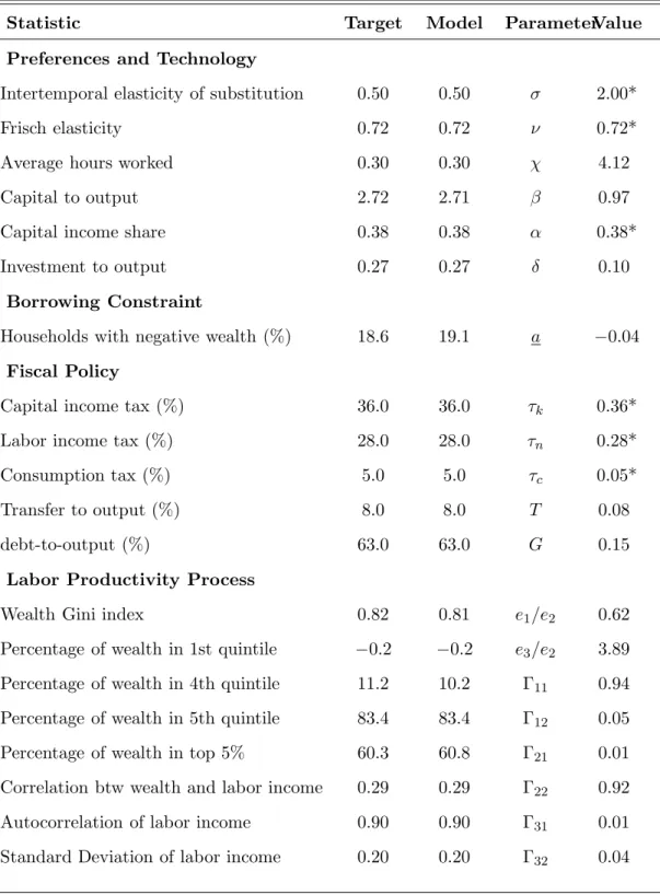
of 15 percent, the data counterpart for the relevant period is approximately 18 percent. Further, we also approximate well the actual income tax schedule as can be seen in Figure 1.2.

Figure 1.2: Income tax schedule

0 2 4 6 8 10 0 2 4 6 8 10

Before Gov. Income

After Gov. Income

45° Data Model

Notes: The data was generously supplied byHeathcote et al.(2014) who used PSID and the TAXSIM program to compute it. The axis units are income relative to the mean.

1.4.4 Labor income process

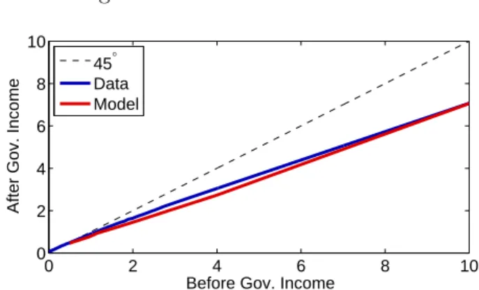
The individual labor productivity levels eand transition probabilities in matrix Γ are chosen to match the US wealth distribution, statistical properties of the estimated labor

(35)

income process and the correlation between wealth and labor income. There are three levels of labor productivity in our model. Since we normalize the average productivity to one we are left with two degrees of freedom. The transition matrix is 3×3. The fact that it is a probability matrix implies its rows add up to one, therefore we are left with an additional six degrees of freedom. Thus, we end up with eight parameters to choose It is common to use the Tauchen method when calibrating the Markov process for productivities. This method imposes symmetry of the Markov matrix which further reduces the number of free parameters. Following Casta˜neda et al. (2003) we do not impose symmetry which allows us to target at the same time statistics from the labor income process and the individual wealth distribution.

To match the wealth distribution we target shares of wealth owned by the first, fourth and fifth quintile, the share of wealth owned by individuals in the top 5 percent and the Gini index. The targets are taken from the 2007 Survey of Consumer Fi-nances22. We also target properties of individual labor income estimated as the AR(1) process, namely its autocorrelation and its standard deviation23. According toDomeij

and Heathcote (2004), existing studies estimate the first order autocorrelation of (log)

labor income to lie between 0.88 and 0.96 and the standard deviation (of the innovation term in the continuous representation) of 0.12 and 0.25. We calibrate the productivity process so that the Markov matrix and vector eimply an autocorrelation of (log) labor income of 0.9 and a standard deviation of 0.224 (in Section 1.7 we provide robustness results with respect to these choices). Finally, we target the correlation between wealth and labor income which is 0.29 in the 2007 SCF data. This way we discipline to some extent the labor income distribution using the wealth distribution that we match accu-rately. The resulting productivity vector, transition matrix and stationary distribution

22_{For a general overview of this data see}_{D´ıaz-Gim´enez et al.}₍₂₀₁₁_).

23_{Including transitory shocks would allow a better match to the labor income process. However, these}

types of shocks can, for the most part, be privately insured against (seeGuvenen and Smith(2013)) so we chose to abstract from them to keep the model parsimonious.

24_{We follow}_Nakajima₍₂₀₁₂_{) in choosing these targets. The targets are associated with labor income,}

wen, which includes the endogenous variableswandn. Therefore, to calibrate the parameters governing the individual productivity process, the model must be solved repeatedly until the targets are satisfied.

(36)

of productivities,λ∗_e, are e=     0.79 1.27 4.94    , Γ =     .956 .043 .001 .071 .929 .000 .012 .051 .937    , and λ ∗ e =     .616 .377 .007    . 1.4.5 Model performance

Table A.1 presents statistics about the wealth and labor income distributions. We tar-get five of the wealth distribution statistics, so it is not surprising that we match that distribution quite well. Table A.2 presents another crucial dimension along which our model is consistent with the data: income sources over the quintiles of wealth. The composition of income, specially of the consumption-poor agents, plays an important role in the determination of the optimal fiscal policy. The fraction of uncertain labor income determines the strength of the insurance motive and the fraction of the unequal asset income affects the redistributive motive. Our calibration delivers, without tar-geting, a good approximation of the income composition. Finally, we also match the consumption Gini which remained fairly constant around 0.27 in the period from 1995 to 2007 (see Krueger and Perri (2006)).

1.5 Main Results

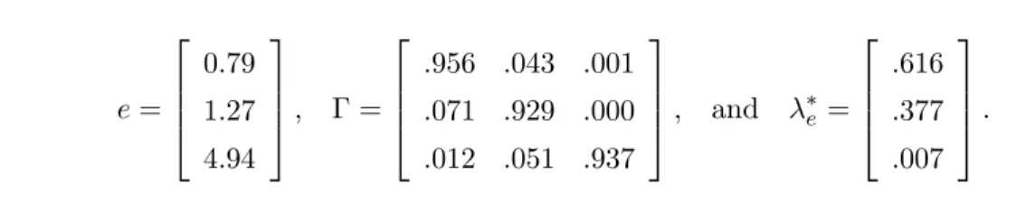
The optimal paths for the fiscal policy instruments are portrayed in Figure1.3. Capital taxes should be front-loaded hitting the upper bound for 33 initial periods then decrease to 45 percent in the long-run. Labor income taxes are substantially reduced to less than half of its initial level, from 28 percent to about 13 percent in the long-run. The ratio of lump-sum transfers to output decreases initially to about 3 percent, then increases back to its initial level of 8 percent before it starts converging to its final level of 3.5 percent. The government accumulates assets in the initial periods of high capital taxes reaching a level of debt-to-output of about −125 percent, which then converges to a final level of −17 percent. Relative to keeping fiscal instruments at their initial levels, this leads to a welfare gain equivalent to a permanent 4.9 percent increase in consumption.

(37)

Figure 1.3: Optimal Fiscal Policy: Benchmark (a) Capital tax

0 20 40 60 80 100 120 0 0.2 0.4 0.6 0.8 1 (b) Labor tax 0 20 40 60 80 100 120 0 0.1 0.2 0.3 (c) Lump-sum-to-output 0 20 40 60 80 100 120 0 0.02 0.04 0.06 0.08 0.1 (d) Debt-to-output 0 20 40 60 80 100 120 −1 −0.5 0 0.5

Notes: Dashed line: initial stationary equilibrium; Solid line: optimal transition; The black dots are the choice variables: the spline nodes andt∗

, the point at which the capital tax leaves the upper bound.

1.5.1 Aggregates

The aggregates associated with the implementation of the optimal policy are shown in Figure A.1. The capital level initially decreases by about 8 percent in the first 13 years, but then increases towards a final level 20 percent higher than the initial steady state. The increase might be surprising at a first glance given the higher capital taxes. First notice that, even if capital income taxes were set to 100 percent forever, there would still be precautionary incentives for the agents with relatively high productivity to save: if they receive a negative shock they can then consume their savings. The decrease in government debt also contributes substantially to this increase - an effect we explain further below in Section 1.5.4. Most importantly though, the level of aggregate labor increases by about 15 percent immediately after the policy change following the reduction in labor taxes, increasing the marginal productivity of capital.

(38)

The higher levels of capital and labor lead to higher levels of output and consump-tion, which increases by 15 and 20 percent respectively over the transition. The concomi-tant increase in average consumption and labor has ambiguous effects on the welfare of the average agent. Hence, we also plot in Figure A.1f what we call the average consumption-labor composite, defined below in equation (1.5.1), which is the more rel-evant measure for welfare. On impact the labor-consumption composite increases by 13 percent as the higher consumption levels (due to the initial reduction in savings) more than compensate for the higher supply of labor. It then decreases for some periods following the reduction in output and the increasing savings. In the long-run it returns to a level about 13 percent higher than the one in the initial steady state.

1.5.2 Distributional Effects

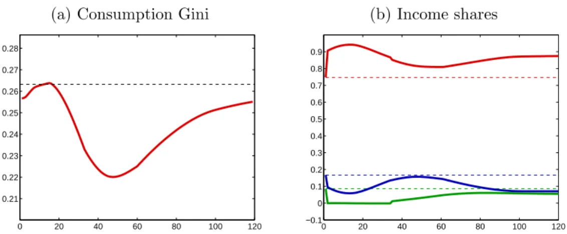
Movements in the levels do not provide a full picture of what results from the imple-mentation of the optimal fiscal policy. It is also important to understand its effects on inequality and on the risk faced by the agents. Figure 1.4a plots the evolution of the Gini index for consumption25_{. Notice that, though it takes some time for the reduction}

to start, the consumption Gini is significantly reduced over the transition reaching a low about 16 percent lower than the initial level. As will become clear below, this reduction in inequality is behind most of the welfare gains associated with the optimal policy. Not surprisingly, such a change would be supported by most agents in the economy with the exception of the highly productive and, therefore, wealthier ones - see Table 1.2.

Figure1.4bdisplays the evolution of the shares of labor, capital and transfer income out of total income. Importantly, notice that the share of labor income is significantly increased under the optimal policy. Since all the risk faced by agents in the SIM model is associated with their labor income, it turns out that they face more risk after the policy is implemented. This has an obvious negative effect on welfare which is, how-ever, outweighed by the gains associated with the higher levels of consumption and the reduction in inequality it provides. The next sections will clarify some of these issues.

25_{Since labor supply is proportional to productivity levels, the inequality of hours is unaffected by}

(39)

Figure 1.4: Inequality measures (a) Consumption Gini

0 20 40 60 80 100 120 0.21 0.22 0.23 0.24 0.25 0.26 0.27 0.28 (b) Income shares 0 20 40 60 80 100 120 −0.1 0 0.1 0.2 0.3 0.4 0.5 0.6 0.7 0.8 0.9

Notes (a) and (b): Dashed lines: initial stationary equilibrium; Solid lines: optimal transition. Notes (b): Red lines: labor income share; Blue lines: transfer income share; Green lines: asset income share

Table 1.2: Proportion in favor of reform

e=L e=M e=H All

99.6 98.3 3.7 99.5

1.5.3 Welfare decomposition

Here we present a result that will be particularly helpful for understanding the properties of the optimal fiscal policy. First, letxtbe the individual consumption-labor composite

(the term inside the utility function 1.4.1), that is

xt≡ct−χ n1+ 1 κ t 1 + 1_κ, (1.5.1)

and Xt denote its aggregate. The utilitarian welfare function can increase for three

reasons. First, it will increase if the utility of the average agent, U({Xt}), increases;

we call this the level effect. Reductions in distortive taxes will achieve this goal by allocating resources more efficiently26. Second, since agents are risk averse, it increases

(40)

if the uncertainty about individual paths {xt}∞_t₌₀ is reduced; we call this the insurance

effect. By redistributing from the (ex-post) lucky to the (ex-post) unlucky, a tax reform can reduce the uncertainty faced by the agents. Finally, it will increase if the inequality across the certainty equivalents of the individual paths{xt}∞t=0, for agents with different

initial (asset/productivity) states, is reduced; we call this the redistribution effect. By redistributing from the rich (ex-ante lucky) to the poor (ex-ante unlucky), the tax reform reduces the inequality between agents. In Appendix A.3we give precise definitions for each of these effects and show how it is possible to measure them. Then, letting ∆ be the average welfare gain, ∆Lthe gains associated with the level effect, ∆I with the insurance

effect, and ∆Rwith the redistribution effect, we prove the following proposition.

Proposition 3 If preferences are GHH as in (1.4.1), then

1 + ∆ = (1 + ∆L) (1 + ∆I) (1 + ∆R).

Hence, it is possible to decompose the average welfare gains into the components described above27_{. The results for this decomposition for our main results are in Table}

1.3. Most of the welfare gains implied by the implementation of the optimal fiscal policy come from the reduction in ex-ante inequality (redistribution effect). The also substantial welfare gains associated with the reduction in distortions (level effect) is almost exactly offset by welfare losses due to the increase in uncertainty (insurance effect).

Table 1.3: Welfare decomposition

Average Level Insurance Redistribution

welfare gain effect effect effect

∆ ∆L ∆I ∆R

4.9 3.7 -3.7 4.9

27_{The welfare gains described above are in terms of consumption-labor composite units. The}

decom-position does not hold exactly in terms of consumption units. To keep our results comparable with others, we report the average welfare gains in terms of consumption units and normalize the numbers for ∆L, ∆I, and ∆Raccordingly.