Joint Validation of Credit Rating PDs under Default Correlation

Full text

(1)

(2) ISSN 1518-3548 CGC 00.038.166/0001-05. Working Paper Series. Brasília. n. 149. Oct. 2007. P. 1-51.

(3) Working Paper Series. Edited by Research Department (Depep) – E-mail: [email protected] Editor: Benjamin Miranda Tabak – E-mail: [email protected] Editorial Assistent: Jane Sofia Moita – E-mail: [email protected] Head of Research Department: Carlos Hamilton Vasconcelos Araújo – E-mail: [email protected] The Banco Central do Brasil Working Papers are all evaluated in double blind referee process. Reproduction is permitted only if source is stated as follows: Working Paper n. 149. Authorized by Mário Mesquita, Deputy Governor for Economic Policy.. General Control of Publications Banco Central do Brasil Secre/Surel/Dimep SBS – Quadra 3 – Bloco B – Edifício-Sede – 1º andar Caixa Postal 8.670 70074-900 Brasília – DF – Brazil Phones: (5561) 3414-3710 and 3414-3567 Fax: (5561) 3414-3626 E-mail: [email protected]. The views expressed in this work are those of the authors and do not necessarily reflect those of the Banco Central or its members. Although these Working Papers often represent preliminary work, citation of source is required when used or reproduced.. As opiniões expressas neste trabalho são exclusivamente do(s) autor(es) e não refletem, necessariamente, a visão do Banco Central do Brasil. Ainda que este artigo represente trabalho preliminar, citação da fonte é requerida mesmo quando reproduzido parcialmente.. Consumer Complaints and Public Enquiries Center Address:. Secre/Surel/Diate Edifício-Sede – 2º subsolo SBS – Quadra 3 – Zona Central 70074-900 Brasília – DF – Brazil. Fax:. (5561) 3414-2553. Internet:. http://www.bcb.gov.br/?english.

(4) Joint Validation of Credit Rating PDs under Default Correlation* Ricardo Schechtman** Abstract. The Working Papers should not be reported as representing the views of the Banco Central do Brasil. The views expressed in the papers are those of the author(s) and do not necessarily reflect those of the Banco Central do Brasil.. The Basel Committee on Banking Supervision recognizes that one of the greatest technical challenges to the implementation of the new Basel II Accord lies on the validation of the banks’ internal credit rating models (CRMs). This study investigates new proposals of statistical tests for validating the PDs (probabilities of default) of CRMs. It distinguishes between proposals aimed at checking calibration and those focused at discriminatory power. The proposed tests recognize the existence of default correlation, deal jointly with the default behaviour of all the ratings and, differently to previous literature, control the error of validating incorrect CRMs. Power sensitivity analysis and strategies for power improvement are discussed, providing insights on the trade-offs and limitations pertained to the calibration tests. An alternative goal is proposed for the tests of discriminatory power and results of power dominance are shown for them with direct practical consequences. Finally, as the proposed tests are asymptotic, Monte-Carlo simulations investigate the small sample bias for varying scenarios of parameters. Keywords: Credit ratings; Probability of default; Validation; Basel II JEL Classification: C12; G21; G28. *. The author would like to thank Axel Munk, Dirk Tasche, Getulio Borges da Silveira and Kostas Tsatsaronis for helpful conversations along the project as well as seminar participants at the Bank for International Settlements (BIS), the 17th FDIC Annual Derivatives Securities and Risk Management Conference, and the C.R.E.D.I.T 2007 Conference. The author also acknowledges the hospitality at the BIS during his fellowship there. Comments and suggestions are welcome. ** Research Department, Banco Central do Brasil. E-mail: [email protected].. 3.

(5) 1. Introduction This paper studies issues of validation for credit rating models (CRMs). In this article, CRMs are defined as a set of risk buckets (ratings) to which borrowers are assigned and which indicate the likelihood of default (usually through a measure of probability of default – PD) over a fixed time horizon (usually one year). Examples include rating models of external credit agencies such as Moody’s and S&P’s and banks’ internal credit rating models. CRMs have had their relevance increased recently as the new Basel II accord (BCBS(2004)) allows the PDs of the internal ratings to function as inputs in the computation of banks’ regulatory levels of capital1. Its goal is not only to make regulatory capital more risk sensitive, and therefore to diminish the problems of regulatory arbitrage, but also to strengthen stability in financial systems through better assessment of borrowers’ credit quality.2 However, the great challenge for Basel II, in terms of implementation, lies on the validation of CRMs, particularly on the validation of bank estimated rating PDs3. In fact, validation of CRMs has been considered a difficult job due to two main factors. Firstly, the typically long credit time horizon of one year or so results in few observations available for backtesting.4 This means, for instance, that the bank/supervisor will, in most practical situations, have to judge the CRM based solely on 5 to 10 (independent) observations available at the database5. Secondly, as borrowers are usually sensitive to a common set of factors in the economy (e.g. industry, geographical region), variation of macro-conditions over the forecasting time horizon induces correlation among defaults. Both these factors contribute to decreasing the power of quantitative methods of validation.. 1. The higher the PD, the higher is the regulatory capital. On top of that, the transparency requirements contained in Basel II can also be seen as an important element aimed at enhancing financial stability. 3 According to BCBS (2005b) validation is above all a bank task, whereas the supervisor’s role should be to certificate this validation. 4 Notice that this problem is not present in the validation of market risk, where the time horizon is typically in the order of days. 5 For statistical standards a small sample. 2. 4.

(6) In light of that picture, BCBS(2005b) perceives validation of CRMs as necessarily comprising a whole set of quantitative and qualitative tools rather than a single instrument. This study focuses solely, however, on a particular set of quantitative tools, namely the statistical tests. Having in mind the aforementioned unavoidable difficulties, this paper scientifically examines the validation of CRMs by means of general statistical tests, not dependent on the particular technique used in their development6. Furthermore, framework to be developed does not aim at a final prescription but at discussing the trade-offs, strategies and limitations involved in the validation task from a statistical perspective. Even restricting to general statistical tests, the judgment of the performance of a CRM is a complex issue. It involves mainly the aspects of calibration and discriminatory power. Calibration is the ability to forecast accurately the ex-post (longrun) default rate of each rating (e.g. through an ex-ante estimated PD). Discriminatory power is the ability to ex-ante discriminate, based on the rating, between defaulting borrowers and non-defaulting borrowers. As BCBS(2004) is explicit about the demand for banks’ internal models to possess good calibration, testing calibration is the starting point of this paper.7 According to BCBS(2005b), quantitative techniques for testing calibration are still on the early stages of development. BCBS(2005b) reviews some simple tests, namely, the Binomial test, the Hosmer-Lemeshow test, a Normal test and the Traffic Lights Approach (Blochwitz et. al. (2003)). These techniques have all the disadvantage of being univariate (i.e. designed to test a single rating PD per time) or to make the unrealistic assumption of cross-sectional default independency8. Further, they do not control for the error of accepting a miscalibrated CRM9. This paper presents an asymptotic framework to jointly test several PDs under the assumption of default correlation and controlling the previous error. The approach is close in spirit to Balthazar (2004), although here the testing problem formulation is remarkably distinct.. 6. This allows the discussions of this paper to assume a general nature. According to BCBS (2004), PDs should resemble long-run average default rates for all ratings. 8 Most of them suffer from both problems. 9 They control for the error of rejecting correct CRMs. 7. 5.

(7) Good discriminatory power is also a desirable property of CRMs as it allows rating based yes/no decisions (e.g. credit granting) to be taken with less error and therefore less cost by the bank (see Blochlinger and Leippold (2006) for instance). BCBS(2005b) comprehensively reviews some well established techniques for examining discriminatory power, including the area under the ROC curve (Engelmann et. al. (2003)), the Accuracy Ratio and the Kolgomorov-Smirnov statistic. Although the use of the above mentioned techniques of discriminatory power is widespread in banking industry, two constraining points should be noted. First, the pursuit of perfect discrimination is inconsistent with the pursuit of perfect calibration in realistic CRMs. The reason is that to increase discrimination one would be interested in having, over the long run, the ex-post rating distributions of the default and non-default groups of borrowers as separate as possible and this involves having default rates as low as possible for good-quality ratings (in particular, lower than the PDs of these ratings) and as high as possible for bad-quality ratings (in particular, higher than the PDs of these ratings). See the appendix A for a graphical example. Second, although not remarked in the literature, usual measures of discriminatory power are function of the cross-sectional dependency between borrowers. This fact potentially represents an undesired property of traditional measures to the extent that the level and structure of default correlation is mainly a portfolio characteristic rather than a property intrinsic to the performance of CRMs10. The framework of this paper leads to theoretical tests of “discrimination power” that 1) can be seen as a necessary requisite to perfect calibration and 2) are not a function of the default dependency structure. This text is organized as follows. Section 2 develops a default rate asymptotic probabilistic model (DRAPM) upon which validation will be discussed. The model leads to a unified theoretical framework for checking calibration and discriminatory power. Section 3 discusses briefly the formulation of the testing problem for CRM validation. The discussion of calibration testing, both one-sided and two-sided, is contained in section 4. Theoretical aspects of discriminatory power testing are. 10. It is not solely a portfolio characteristic because default correlation among the ratings potentially depends on the design of the CRM too.. 6.

(8) investigated in section 5. Section 6 contains a Monte–Carlo analysis of the small sample properties of DRAPM and their consequences for calibration testing. Section 7 concludes.. 2. The default rate asymptotic probabilistic model (DRAPM) The model of this section provides a default rate probability distribution upon which statistical testing is possible. It is based on an extension of the Basel II underlying model of capital requirement. In fact, this paper generalizes the idea of Balthazar(2004), of using the Basel II model for validation, to a multi-rating setting11,12. The applied extension is based on Demey et. al. (2004)13 and refers to including an additional systemic factor for each rating. While in Basel II the reliance on a single factor is crucial to the derivation of portfolio invariant capital requirements (c.f. Gordy (2003)), for validation purposes a richer structure is necessary to allow for non-singular variance matrix among the ratings, as it becomes clearer ahead in the section. The formulation of DRAPM starts with a decomposition of zin, the normalized return on assets of a borrower n with rating i. Close in spirit to Basel II model, zin is expressed as: zin = ρB½ x + (ρW - ρB)½ xi + (1- ρW )½ εin, for each rating i=1…I and each borrower n=1..N, where x, xi, εij (i=1...I, j=1…N) are independent and standard normal distributed. Above, x represents a common systemic factor affecting the asset return of all borrowers, xi a systemic factor affecting solely the asset return of borrowers with rating i and εin an idiosyncratic shock. The parameters ρB and ρW lie in the interval [0 1]. Note. 11. This paper’s approach also differs from Balthazar(2004) in reversing the role of the hypothesis, as section 3 explains. 12 The reader is referred to BCBS(2005a) for a detailed presentation of the Basel II underlying model. 13 The purpose of Demey et. al. (2004) is to estimate correlations while the focus here is on developing a minimal non-degenerate multivariate structure useful for testing.. 7.

(9) that Cov(zin,zjm) is equal to ρW if i=j and to ρB otherwise, so that ρW represents the “within-rating” asset correlation and ρB the “between-rating” asset correlation. The model description continues with the statement that a borrower j with rating i defaults at the end of the forecasting time horizon if zin < Φ-1(PDi) at that time, where Φ denotes the standard normal cumulative distribution function. Note that the probability of this event is therefore, by construction, PDi14. Consequently, the conditional probability of default PDi(x), where x=(x,x1,…,xI)’ denotes the vector of systemic factors, can be expressed by: PDi(x) ≡ Prob(zin < Φ-1(PDi)|x) = Φ( (Φ-1(PDi) - ρB½ x - (ρW - ρB)½ xi )/(1- ρW )½ ). Let’s focus now on the asymptotic behaviour of the observable default rates. Let DRiN denote the default rate computed using a sample of N borrowers with rating i at the start of the forecasting horizon. It is easy to see, as in Gordy (2003), that: DRiN – E(DRiN|x) ≡ DRiN – PDi(x) → 0 a.s. when N → ∞15 Therefore, as Φ-1 is continuous, it is also true that Φ-1(DRiN) – Φ-1(PDi(x)) → 0 a.s. when N → ∞, so that in DRAPM the Φ-1 transformed default rates have asymptotically the same distribution as the Φ-1 transformed conditional probabilities, which are normal distributed16,17. More concretely, the limiting default rate joint distribution is: Φ-1(DR) ≈ N(μ, ∑) where DR = (DR1,DR2,…,DRI)T, μi = Φ-1(PDi)/(1- ρW )½ , ∑ij = ρW /(1- ρW) if i=j and ∑ij =ρB /(1- ρW) otherwise.. 14. Without generalization loss, PDi is assumed to increase in i. a.s. stands for almost sure convergence. 16 See the expression for PD(x). 15. 8.

(10) This is the distribution upon which all the tests of this paper will be derived. A limiting normal distribution is mathematically convenient to the derivation of likelihood ratio multivariate tests. The cost to be paid is that the approach is asymptotic, so that the discussions and results of this paper are not suitable for CRMs with a small number of borrowers per rating, such for example rating models for large corporate exposures. Even for moderate numbers of borrowers, section 6 reveals that the departure from the asymptotic limit can be substantial, significantly altering the theoretical size and power of the tests. Application of the tests of the next sections should then be extremely careful. Some comments on the choice of the form of ∑ are warranted18. To the extent that borrowers of each rating present similar distributions of economic and geographic sectors of activity, that define the default dependency, ρB is likely to be very close to ρW, as this situation resembles the one factor case. By its turn, this paper assumes 0 < ρB < ρW, in opposition to ρB = ρW, in order to leave open the possibility of some degree of association between PDs and borrowers’ sectors of activity and with the technical purpose of obtaining a non-singular matrix ∑19,20. As a result, borrowers in the same rating behave more dependently than borrowers in different ratings, possibly because the profile of borrowers’ sectors of activity is more homogeneous within than between ratings. Indeed, more realistic modelling is likely to require a higher number of asset correlation parameters and a portfolio dependent approach; therefore the choice of just a pair of correlation parameters is regarded here as a practical compromise for general testing purposes. This paper further assumes that the correlation parameters ρW and ρB are known. The typically small number of years that banks have at their disposal suggests that the. 17. Although the choice of the normal distribution for the systemic factors may seem arbitrary in Basel II, for the testing purposes of this paper it is a pragmatic choice. 18 Note that the structure of ∑ defines DRAPM more concretely than the chosen decomposition of the normalized asset return, because the decomposition is not unique given ∑. 19 To the best of the author’s knowledge, the empirical literature lacks studies on that association. 20 Even if the bank or the supervisor is convinced of the appropriateness of ρB = ρW, the approach of this paper is still defendable, provided, for instance, the default rates of different ratings are computed based on distinct sectors of activity.. 9.

(11) inclusion of correlation estimation in the testing procedure is not feasible, as it would diminish considerably the power of the tests. Instead, this paper relies on Basel II accord to extract some information on correlations21. By matching the variances of the nonidiosyncratic parts of the asset returns in Basel II and DRAPM models, ρW can be seen as the asset correlation parameter present in the Basel II formula22. For corporate borrowers, for example, Basel II accord chooses ρW ∈ [0.12 0.24] 23. Sensitivity analysis of the power of the tests on the choices of these parameters is carried out in section 4. It should be noted, however, that the supervisory authority may have a larger set of information to estimate correlations and/or may even desire to set their values publicly for testing purposes. Finally, it is assumed serial independency for the annual default rate time series. Therefore, the (Φ-1 transformed) average annual default rate, used as the test statistic for the tests of the next sections, has the normal distribution above, with ∑/Y in place of ∑, where Y is the number of years available to backtest. According to BCBS(2005b), serial independency is less inadmissible than cross-sectional independency.. 3. The formulation of the testing problem Any configuration of a statistical test should start with the definitions of the null hypothesis Ho and the alternative one H1. In testing a CRM, a crucial decision refers to where the hypothesis “the rating model is correctly specified” should be placed?24 If the bank/supervisor only wishes to abandon this hypothesis if data strongly suggests it is false then the “correctly specified” hypothesis should be placed under H0,. 21. An important distinction to the Basel II model, however, is that this paper does not make correlations dependent on the rating. In fact, the empirical literature on asset correlation estimation contains ambiguous results on this sensitivity. 22 Note that Basel II can also be seen as the particular case of DRAPM when the coefficient of xi is null, i.e. when ρB = ρW. 23 On the other hand, Basel II accord doesn’t provide information on ρB because it is based on a single systemic factor. 24 For this general discussion, one can think of “correctly specified” as meaning either correct calibration or good discriminatory power.. 10.

(12) as in BCBS (2005b) or in Balthazar (2004)25. But if the bank/supervisor wants to know if the data provided enough evidence confirming the CRM is correctly specified, then this hypothesis should be placed in H1 and its opposite in Ho. The reason is that the result of a statistical test is reliable knowledge only when the null hypothesis is rejected, usually at a low significance level. The latter option is pursued throughout this paper. Thus the probability of accepting an incorrect CRM will be the error to be controlled for at the significance level α. To the best of the author’s knowledge this paper is the first to feature the CRM validation problem in this way. Placing the “correctly specified” hypothesis under H1 has immediate consequences. For a statistical test to make sense H0 usually needs to be defined by a closed set and H1, therefore, by an open set26. This implies that the statement that “the CRM is correctly specified” needs to be translated into some statement about the parameters PDis lying in an open set, in particular there shouldn’t be equalities defining H1 and the inequalities need to be strict. It is, for example, statistically inappropriate to try to conclude that the PDis are equal to the bank postulated values. In cases like that the solution is to enlarge the desired conclusion by means of the concept of an indifference region. The configuration of the indifference region should convey the idea that the bank/regulator is satisfied with the eventual conclusion that the true PD vector lies there. In the previous case the indifference region could be formed for example by open intervals around the postulated PDis. The next sections make use of the concept to a great extent. At this point it is desirable only to remark that the feature of an indifference region shouldn’t be seen as a disadvantage of the approach of this paper. Rather, it reflects better the fact that not necessarily all the borrowers in the same rating i have exactly the same theoretical PDi and that it is, therefore, more realistic to see the ratings as defined by PD intervals.27. 25. Although they do not remark the consequences of this choice. H0 and H0 U H1 need to be closed sets in order to guarantee that the maximum of the likelihood function is attained. 27 However, in the context of Basel II, ratings need not be related to PD intervals but merely to single PD values. In light of this study’s approach, this represents a gap of information needed for validation. 26. 11.

(13) 4. Calibration testing This section distinguishes between one-sided and two-sided tests for calibration. One-sided tests (which are only concerned about PDis being sufficiently high) are useful to the supervisory authority by allowing to conclude that Basel II capital requirements derived by the approved PD estimates are sufficiently conservative in light of the banks’ realized default rates. From a broader view, however, not only excess of regulatory capital is undesirable by banks but also BCBS(2004) states that the PD estimates should ideally be consistent with the banks’ managerial activities such as credit granting and credit pricing28. To accomplish these goals, PD estimates must, without adding distortions, reflect the likelihood of default of every rating, something to be verified more effectively by two-sided tests (which are concerned about PDis being within certain ranges). Unfortunately the difficulties present in two-sided calibration testing are greater than in one-sided testing, as indicated ahead in the section. The analysis of onesided calibration testing starts the section. 4.a. One-sided calibration testing Based on the arguments of the previous section about the proper roles of Ho and H1, the formulation of a one-sided calibration test is proposed below. Note that the desired conclusion, configured as an intersection of strict inequalities, is placed in H1. Ho: PDi ≥ ui for some i =1…I H1: PDi < ui for every i=1…I where PDi ≡ Φ-1(PDi) , ui ≡ Φ-1 (ui). (This convention of representing Φ-1 transformed figures in italic is followed throughout the rest of the text)29.. 28. More specifically, if the PDs used as inputs to the regulatory capital differ from the PDs used in managerial activities, at least some consistency must be verified between the two sets of values for validation purposes, c.f. BCBS(2006). 29 As Φ-1 is strictly increasing, statements about italic figures imply equivalent statements about non-italic figures.. 12.

(14) Here ui is a fixed known number that defines an indifference acceptable region for PDi. Its value should ideally be slightly larger than the value postulated for PDi so that the latter is within the indifference region. Besides, ui should preferably be smaller than the value postulated for PDi+1 so that at least the rejection of H0 could conclude that PDi < postulated PDi+1.30,31 According to DRAPM and based on the results of Sasabuchi (1980) and Berger (1989), which investigate the problem of testing homogeneous linear inequalities concerning normal means, a size α critical region can be derived for the test.32 Reject H0 (i.e. validate the CRM) if. DR i ≤ ui /(1- ρW )½ - zα (ρW /(Y(1- ρW))) ½ for every i = 1…I Y. where DR i =. ∑ DR. iy. y =1. Y. is the (transformed) average annual default rate of rating i. and zα = Φ(1-α) is the 1-α percentile of the standard normal distribution.33 This test is a particular case of a min test, a general procedure that calls for the rejection of a union of individual hypotheses if each one of them is rejected at level α. In general the size of a min test will be much smaller than α but the results of Sasabuchi (1980) and Berger (1989) guarantee that the size is exactly α for the previous one-sided calibration test34. This means that the CRM is validated at size α if each PDi is validated as such. A min test has several good properties. First, it is uniformly more powerful (UMP) among monotone tests (Laska and Meisner (1989)), which gives a solid theoretical foundation for the procedure since monotonicity is generally a desired. 30. As banks have the capital incentive to postulate lower PDs one could argue that PDi < postulated PDi+1 also leads to PDi < true PDi+1. 31 Specific configurations of ui are discussed later in the section. 32 Size of a test is the maximum probability of rejecting H0 when it is true. 33 This definition of DR i is used throughout the paper. 34 More formally this is the description of a union-intersection test, of which the min test is a particular case when all the individual critical regions are intervals not limited on the same side.. 13.

(15) property.35 Second, as the transformed default rate variables are asymptotically normal in DRAPM, the min test is also asymptotically the likelihood ratio test (LRT). Finally, the achievement of size α is robust to violation of the assumption of normal copula for the transformed default rates (Wang et. al. (1999)) so that, for size purposes, the requirement of joint normality for the systemic factors can be relaxed. From a practical point of view it should be noted that the decision to validate or not the CRM does not depend on the parameter ρB, which is useful for applications since ρB is not present in Basel II framework and so there is not much knowledge about its reasonable values. However, the power of the test, i.e. the probability of validating the CRM when it is correctly specified, does depend on ρB. The power is given by the expression below. Power = ΦI(- zα + (u1 – PD1)/ (ρW /Y) ½,….,-zα + (ui – PDi)/ (ρW /Y) ½ , ….,-zα + (uI – PDI)/ (ρW /Y) ½, ρB /ρW ),. where ΦI(….,ρB /ρW) is the cumulative distribution function of a Ith-variate normal of mean 0, variances equal to 1 and covariances equal to ρB/ρW. Berger (1989) remarks that if the ratio ρB /ρW is small then the power of this test can be quite low for the PDis only slightly smaller than uis and/or a large number of ratings I. This is intuitive as a low ratio ρB/ρW indicates that ex-post information about one rating does not contain much information about other ratings and so is less helpful to conclude for validation. On the other hand, as previously noted in section 2, DRAPM is more realistic when ρB/ρW is close to 1 so that the referred theoretical problem becomes less relevant in the practical case. More generally, it is easy to see that the power increases when PDis decrease, uis increase, Y increases, I decreases, ρB increases or ρW decreases36. In fact, it is worth examining the trade-off between the configuration of the indifference region in the form. 35. In the context of this paper, a test is monotone if the fact that average annual default rates are in the critical region implies that smaller average default rates are still in the critical region. Monotonicity is further discussed later in the paper. 36 Obviously the power also increases when the level α increases.. 14.

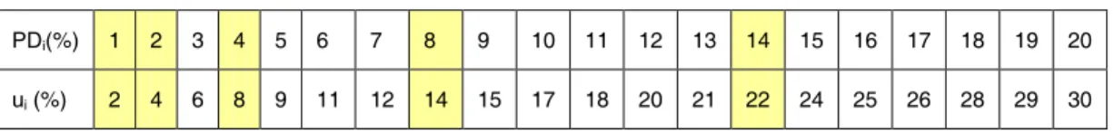
(16) of the uis and the attained power. If high precision is demanded (uis close to postulated PDis) then power must be sacrificed; if high power is demanded then precision must be sacrificed (uis far from postulated PDis). Some numerical examples are analyzed below in order to provide further insights on this trade-off. The case I=1 represents an upper bound to the power expression above. In this case, for a desired power of β when the probability of default is exactly equal to the postulated PD, it is true that:. u – PD = (zα - zβ )× (ρW /Y) ½ In a base case scenario given by Y=5, ρW = 0.15, α = 15 % and β = 80 % the right hand side of the previous equation is approximately equal to 0.32. This scenario is considered here sufficiently conservative with a realistic balance between targets of power and size. In this case, it holds that: ui = Φ(0.32 + Φ-1(PDi)) Table 1 below displays pairs of values of ui and PDi that conform to the equality above. Table 1: ui X PDi. PDi(%). 1. 2. 3. 4. 5. 6. 7. 8. 9. 10. 11. 12. 13. 14. 15. 16. 17. 18. 19. 20. ui (%). 2. 4. 6. 8. 9. 11. 12. 14. 15. 17. 18. 20. 21. 22. 24. 25. 26. 28. 29. 30. As, in a multi-rating context, any reasonable choice of ui must satisfy ui ≤ PDi+1, table 1 illustrates, for the numbers of the base case scenario, an approximate lower bound for PDi+1 in terms of PDi37,38. More generally, table 1 provides examples of whole rating scales that conform to the restriction PDi+1 ≥ ui, e.g. PD1=1%, PD2=2%, PD3=4%, PD4=8%, PD5=14%, PD6=22%, PD7=36%. Note that such conforming rating. 37. Approximate because the computation was based on I=1. In fact the true attained power in a multi rating setup is smaller. 38 The discussion of this paragraph assumes true PD = postulated PD.. 15.

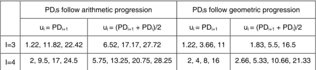
(17) scales must posses increasing PD differences between consecutive ratings (i.e. PDi+1 PDi increasing in i), a characteristic found indeed in the design of many real-world CRMs. Therefore DRAPM suggests a validation argument in favour of that design choice. Notice that this feature of increasing PD differences is directly related to the non-linearity of Φ, which in turn is a consequence of the asymmetry and kurtosis of the distribution of the untransformed default rate. To further investigate the feature of increasing PD differences and choices of u=(u1,u2,…,uI)’ in the one-sided calibration test, the cases I=3 and I=4 are explicitly analyzed in the sequence. For each I, four CRMs are considered with their PDis depicted in table 2. CRMs of table 2 can have PDis following either an arithmetic progression or a geometric progression. Besides, two strategies of configuration of the indifference region are considered: a liberal one with ui = PDi+1 and a more precise one with ui = (PDi+1 + PDi)/2. In order to allow for a fair comparison of power among distinct CRMs, PDis figures of table 2 are chosen with the purpose that the resulting sets of ratings of each CRM cover equal ranges in the PD scale. More specifically, this goal is interpreted here as all CRMs having equal u0 and uI39,40. Table 2: PDs(%) chosen according to ui specification and CRM design PDis follow arithmetic progression. PDis follow geometric progression. ui = PDi+1. ui = (PDi+1 + PDi)/2. ui = PDi+1. ui = (PDi+1 + PDi)/2. I=3. 1.22, 11.82, 22.42. 6.52, 17.17, 27.72. 1.22, 3.66, 11. 1.83, 5.5, 16.5. I=4. 2, 9.5, 17, 24.5. 5.75, 13.25, 20.75, 28.25. 2, 4, 8, 16. 2.66, 5.33, 10.66, 21.33. The power figures of the one-sided calibration test at the postulated PDs are shown in tables 3 and 4, according to values set to parameters ρW and Y. The values of these parameters are chosen considering three feasible scenarios: a favourable one characterized by 10 years of data and a low within-rating correlation of 0.12, a. 39. u0 corresponds to the fictitious PDo. At table 2, PDo can be easily figured out from the constructional logic of the PDi progression. 40 For the construction of the CRMs of table 2, u0=1.22% and u3=33% for I=3 and u0=2% and u4=32% for I=4. Furthermore the ratio of the PDi geometric progression is set equal to 3 for I=3 and to 2 for I=4.. 16.

(18) unfavourable one characterized by the minimum number of 5 years prescribed by Basel II (c.f.Basel (2004)) and a high ρW at 0.18 and an in-between scenario41. Table 3: Power comparison among CRM designs and ui choices, I=3 ρB/ρW = 0.8, α= 0.15 PDis follow arithmetic progression. PDis follow geometric progression. ui = PDi+1. ui = (PDi+1 + PDi)/2. ui = PDi+1. ui = (PDi+1 + PDi)/2. ρW = 0.12, Y=10. 0.97. 0.57. 0.99. 0.95. In-between. 0.85. 0.42. 0.97. 0.81. ρW =0.18, Y=5. 0.72. 0.33. 0.91. 0.67. Table 4: Power comparison among CRM designs and ui choices, I=4 ρB/ρW = 0.8, α= 0.15 PDis follow arithmetic progression. PDis follow geometric progression. ui = PDi+1. ui = (PDi+1 + PDi)/2. ui = PDi+1. ui = (PDi+1 + PDi)/2. ρW = 0.12, Y=10. 0.82. 0.39. 0.95. 0.68. In-between. 0.62. 0.28. 0.81. 0.48. ρW =0.18, Y=5. 0.49. 0.22. 0.65. 0.37. Table 3 and 4 show that CRMs with the feature of increasing (PDi+1 - PDi) usually achieve significantly higher levels of power than CRMs with equally spaced PDis, confirming the intuition derived from table 1. The tables also reveal that, even when solely focusing on the former, more demanding requirements for ui (c.f. ui = (PDi+1 + PDi)/2) may produce overly conservative tests, with for example power on the level of only 37%. Therefore liberal strategies for ui (c.f. ui = PDi+1) seem to be necessary for realistic validation attempts and attention is focused on these strategies to the remainder of this section. Further from the tables, the power is found to be very sensitive to the within-rating correlation ρW and to the number of years Y. It can increase more than 80% from the worst to the best scenario (c.f. last column of table 4).. 41. As ρB/ρW is fixed in tables 3 and 4, what matters for the power calculation is just the ratio (ρW/Y). Therefore, the in-between scenario can be thought as characterized by adjusting both Y and ρW or just one of them. At tables 3 and 4 it is given by (ρW/Y) ½ = 0.15.. 17.

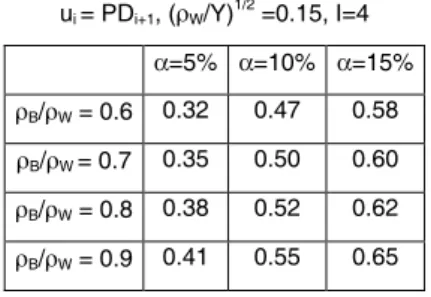
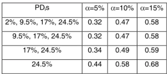
(19) While in previous tables the between-rating correlation parameter ρB is held fixed, tables 5 and 6 examine its effect, along a set of feasible values, on the power of the test. Power is computed at the postulated PDs of CRMs of table 2 with ui = PDi+1, I=4 and for the in-between scenario of parameters of ρW and Y. The tables show just a minor effect of ρB, regardless of the size of the test and the CRM design. Therefore, narrowing down the uncertainty in the value of ρB value is not of great importance if just approximate levels of power are desired at postulated PDs. The elements that indeed drive the power of the test are unveiled in the next analysis. Table 5: Effect of ρB when PDis follow arithmetic progression ui = PDi+1, (ρW/Y)1/2 =0.15, I=4 α=5% α=10% α=15% ρB/ρW = 0.6. 0.32. 0.47. 0.58. ρB/ρW = 0.7. 0.35. 0.50. 0.60. ρB/ρW = 0.8. 0.38. 0.52. 0.62. ρB/ρW = 0.9. 0.41. 0.55. 0.65. Table 6: Effect of ρB when PDis follow geometric progression ui = PDi+1, (ρW/Y)1/2 =0.15, I=4 α=5% α=10% α=15% ρB/ρW = 0.6. 0.54. 0.69. 0.78. ρB/ρW = 0.7. 0.56. 0.71. 0.79. ρB/ρW = 0.8. 0.60. 0.73. 0.81. ρB/ρW = 0.9. 0.62. 0.74. 0.82. Tables 7 and 8 below provide insights on the relative role played by the different ratings on the power. Power is computed at postulated PDs for a sequence of four embedded CRMs, starting with the CRM with equally spaced PDs of the second line of table 7 (the CRM with increasing PD differences of the second line of table 8). Each next CRM in table 7 (table 8) is built from its antecedent by dropping the less risky (riskiest) rating. Power is computed for the in-between scenario and ui = PDi+1. The tables reveal that, as the number of ratings diminishes, the power increases just to a minor extent, provided the riskiest (less risky) ratings are always kept in the CRM. Thus it can be said that in table 7 (table 8) the highest (lowest) PDis drive the power of the test. This is partly intuitive because the highest (lowest) PDis correspond to the smallest differences (ui - PDi) in the CRMs of table 7 (table 8) and because distinct PDis. 18.

(20) contribute to the power differently just to the degree their differences (ui - PDi) vary42. The surprising part of the result refers to the degree of relative low importance of the dropped PDis: the variation of power between I=1 and I=4 can be merely around 10%. This latter observation should be seen as a consequence of the functional form of DRAPM, particularly the choice of the normal copula for the (transformed) default rates and the form of Σ. Table 7: Influence of distinct PDis on power PDis follow arithmetic progression; ρB/ρW = 0.6; (ρW /Y) ½ = 0.15; ui = PDi+1 α=5% α=10% α=15%. PDis 2%, 9.5%, 17%, 24.5%. 0.32. 0.47. 0.58. 9.5%, 17%, 24.5%. 0.32. 0.47. 0.58. 17%, 24.5%. 0.34. 0.49. 0.59. 24.5%. 0.44. 0.58. 0.68. Table 8: Influence of distinct PDis on power PDis follow geometric progression; ρB/ρW PDis. ½. = 0.6; (ρW /Y) = 0.15; ui = PDi+1. α=5% α=10% α=15%. 2%, 4%, 8%, 16%. 0.54. 0.69. 0.78. 2%, 4%, 8%. 0.54. 0l.69. 0.78. 2%, 4%. 0.56. 0.71. 0.79. 2%. 0.65. 0.77. 0.84. A message embedded in the previous tables is that in some quite feasible cases (e.g. Y=5 years available at the database, ρW = 0.18 reflecting the portfolio default volatility, α < 15% desired) the one-sided calibration test can have substantially low power (e.g. lower than 50% at the postulated PD). Another related problem refers to the test not being similar on the boundary between the hypotheses and therefore biased (if I>1)43. To cope with these deficiencies, the statistical literature contains some proposals. 42. It is easy to see that for the CRMs with equally spaced PDis, (ui – PDi) is trivially constant in i but the Φ-1-transformed difference (ui – PDi) decreases in i. For the CRMs with increasing (PDi+1 – PDi,), (ui – PDi) trivially increases in i and the Φ-1-transformed difference (ui – PDi) increases in i too. 43 A test is α similar on a set A if the probability of rejection is equal to α everywhere there. A test is unbiased at level α if the probability of rejection is smaller than α everywhere in H0 and greater than α everywhere in H1. Every unbiased test at level α with a continuous power function is α-similar in the boundary between H0 and H1. (Gourieroux & Monfort (1995)). 19.

(21) of non-monotone uniformly more powerful tests for the same problem, such as in Liu and Berger (1995) and Dermott and Wang (2002). The new tests are constructed by carefully enlarging the rejection region in order to preserve the size α. The enlargement trivially implies power dominance. The new tests have two main disadvantages though. First, from a supervisory standpoint, non-monotone rejection regions are harder to defend on an intuitive basis because they imply that a bank could pass from a state of validated CRM to a state of non-validated CRM if default rates for some of the ratings. decrease. Second, from a theoretical point of view, Perlman and Wu (1999) note that the new tests do not dominate the original test in the decision theoretic sense because the probability of validation under H0 (i.e. when the CRM is incorrect) is also higher for them44. The authors conclude that UMP tests should not be pursued at any cost, particularly at the cost of intuition. This is the view adopted in this study so that the new tests are not explored further in this paper. Yet, one may try to include some prior knowledge in the formulation of the onesided calibration test as a strategy for power improvement. Notice, first, that the size α of the test is attained when all but one of the PDis go to 0 while the remaining one is set fixed at ui45,46. This is probably a very unrealistic scenario against which the bank or the supervisor would like to be protected. The bank/supervisor may alternatively remove by assumption this unrealistic case from the space of PD possibilities and rather consider that part of the information to be tested is true. Notably, it can be assumed that the postulated PDi-1, not 0, represents a lower bound for PDi, for every rating i. A natural modification of the test consists then on replacing zα by a smaller constant c > 0 to adjust to the removed unrealistic PD scenarios47, with resulting enlargement of the critical region and achievement of a more powerful test48. Hence, c is defined by the requirement that the size of the modified test (with c instead of zα) in the reduced PD space is α. Similarly to Sasabuchi (1980), the determination of c needs the examination. 44. More specifically, the power is higher at every PD parameter in H0. This limiting PD vector is in H0 and, therefore, should not be validated. It has a probability of validation equal to α. 46 Note PDi → 0 ⇒ PDi → -∞ 47 As the coordinates of the input to the power function cannot go to infinity as before, -c > -zα for the size to be achieved. 48 See the definition of the critical region in the beginning of the section. 45. 20.

(22) of only the PD vectors with all but one of their coordinates PDis equal to their lower bounds (the postulated PDi-1s), and the remaining one, say PDj, set at uj, for j varying in 1…I. More formally, Max 1≤j≤I (ΦI(-c + (u1 – PD0)/ (ρW /Y) ½ , ….,-c, …,-c + (uI – PDI-1)/ (ρW /Y) ½ ; ρB /ρW ) = α49,50,. from which the value of c can be derived. However, produced results indicate the previous modification approach is of limited efficacy to power improvement. More specifically, computed results indicate that the power increase is relevant only in the region of small (probably unrealistic) ratio ρB/ρW or for ambitious choices of ui (i.e. close to PDi). In the latter case, the increase is not sufficient, however, to the achievement of reasonable levels of power because the original levels are already too low (c.f. table 1 for example). Those results are consistent with the intuition derived from the analysis of tables 7 and 8. On the other hand, one may also try to derive the LRT based on the restricted PD parameter space: Ho: PDi ≥ ui for some i =1…I and PDi ≥ postulated PDi-1 for every I=1…I51 H1: PDi < ui for every i=1…I and PDi ≥ postulated PDi-1 for every I=1…I52 The LRT will differ from the modification approach with respect to the information contained in the observed default rates. The LRT will have very small observed average default rates providing lower relative evidence in favour of H1, because, by assumption, they cannot be explained by very small PDs53. Accordingly, the null distribution of the likelihood ratio (LR) statistic doesn’t need to put mass on those unrealistic PD scenarios. Unfortunately, to the best of the author’s knowledge, the derivation of the LRT critical region for such a problem is lacking in the statistical. 49. PD0 is here just a lower bound to PD1. It could be -∞ or defined subjectively based on accumulated practical experience. 50 Note that the new critical region will now depend on ρB and that the calculation of c needs some computational effort. 51 Same observation about PD0 applies here as well. 52 H1 need not be defined only by strict inequalities here since the union H0 U H1 does not span the full |RI.. 21.

(23) literature. Its complexity arises from the facts that, in contrast to the original one-sided calibration test, H0 and H1 do not share the same boundary in |RI and that the boundary indeed shared is a limited set. Thus, it is reasonable to conjecture that the null distribution of the LR statistic will be fairly complicated. And similarly to the previous strategy, if ui >> postulated PDi-1 for most ratings, the increase in power is likely to negligible again54. 4.b. Two-sided calibration testing The section now comments on two-sided calibration testing, mostly from a theoretical perspective. Similarly to the one-sided version, the hypotheses of a twosided test can be stated as follows. Ho: PDi ≥ ui or PDi ≤ li for some i =1.. I H1: li < PDi < ui for every i=1…I Now the acceptable indifference region is defined by two parameters ui and li for each rating i, with ideally li ≥ postulated PDi-1 and ui ≤ postulated PDi+1. Under that formulation, the test belongs to the class of multivariate equivalence tests, which are tests designed to show similarity rather than difference and are widely employed in the pharmaceutical industry to demonstrate that drugs are equivalent.55 Berger and Hsu (1996) comprehensively review the recent development of equivalence tests in the univariate case (I=1). The standard procedure to test univariate equivalence is the TOST test (two one-sided tests - called this way because the procedure is equivalent to performing two size-α one sided tests and concluding equivalence only if both reject). Wang et.al. (1999) discuss the extension of TOST to the multivariate case, making use. 53. Very small observed average default rates in the sense that Φ-1(DRi)/(1- ρW )½ < Φ-1(postulated PDi-1). It is important to remark that if I is large, strategies of power improvement will generally have more chances of relative success, although they depart from lower original levels of power. 55 More specifically, those tests are referred as bioequivalent tests in the pharmaceutical industry. 54. 22.

(24) of the intersection-union method56. When applied to the DRAPM distribution, that extension results in the following critical region for the two-sided calibration test57. Reject Ho (i.e. validate the CRM) if li /(1- ρW )½ + zα (ρW /(Y(1- ρW))) ½ ≤ DR i ≤ ui /(1- ρW )½ - zα (ρW /(Y(1- ρW))) ½ ,. for every i = 1…I As the maximum power of the test occurs in the middle point of the cube [li ui]I, it is reasonable to make the cube symmetric around the postulated PD (in other words, to make ui - PDi = PDi - li for every i), so that the highest probability of validating the CRM occurs exactly at the postulated PD. Additional configurations of the indifference region may include, as in the one-sided test, choosing ui = PDi+1 or li=PDi-1 (but not both). Similarly to the one-sided test, the two-sided version has similar problems of lack of power and bias58. In this respect, the statistical literature contains some proposals for improving TOST (Berger and Hsu(1996), Brown et. al.(1998)), which are again subject to criticism from an intuitive point of view by Perlman and Wu (1999)59. Furthermore, an additional drawback of the two-sided test, in contrast to the original TOST, is its excess of conservatism because the test is only level α while its size may be much smaller.60,61 That observation indicates the magnified difficulty in performing two-sided calibration testing. Yet, two additional approaches to testing multivariate equivalence deserve comments. The first one is developed by Brown et. al.(1995). Applied to the problem of. 56. Wang et. al. (1999) also show that TOST is basically a LR test. The standard TOST is formulated assuming unknown variance while the proposed two-sided calibration test of this paper assumes known variance. Therefore the reference to the term TOST encompasses here some freedom of notation. 58 If I>1, the test is not similar on the boundary between the hypotheses and therefore biased. 59 However, in the case of calibration testing with known variance, the bias is not as pronounced as in the standard TOST with unknown variance due to the impossibility of making the variance go to 0 as in Berger and Hsu (1996). 60 It can be shown that the degree of conservatism depends on ρB. 61 The reason for the discrepancy with the standard TOST relates again to the impossibility of making the variance go to 0 as in Berger and Hsu (1996). 57. 23.

(25) PD calibration testing, it consists of accepting an alternative hypothesis H1 (i.e. validating the CRM) if the Brown confidence set for the PD vector is entirely contained in H1. The approach would allow the bank or the supervisor to separate the execution of the test from the task of defining an indifference region because H1 configuration could be discussed at a later stage, after the knowledge of the form of the set. In particular, the confidence set can be seen as the smallest indifference region that still permits to validate the calibration. Brown et.al. (1995) propose an optimal confidence set in the sense that, if the true PD vector is equal to the postulated one, then the expected volume of that set is minimal, which means that, in average terms, maximal precision is achieved when calibration is exactly right62. The cost of this optimality is larger set volumes for PDs different from the postulated one. Munk and Pfluger (1999) show in simulation exercises that the power of Brown’s procedure can be substantially lower than those of more standard tests, like the TOST, for a wide range of PDs close to the postulated one. Therefore, in light of the view of this paper that ratings could more realistically be seen as PD intervals, the benefit of the optimality at a single point is doubtful at a minimum. Consequently, Brown’s approach is regarded here as of more theoretical than practical value to calibration testing.63,64 The second different approach to testing multivariate equivalence is developed by Munk and Pfluger (1999). So far, this paper has just considered rectangular sets in the H1 statements of the calibration tests. The goal has been to show that the true PD lies in a rectangle or in quadrant of the space |RI. The referred authors analyze instead the use of ellipsoidal alternatives for the multivariate equivalence problem, which, for purposes of calibration testing, can be exemplified as follows. Ho: etDe ≥ Δ H1: etDe < Δ. 62. The form of the set is not an ellipse, commonly found in multivariate analysis, but rather a figure known as the Limaçon of Pascal. 63 Note also that DRAPM should be seen just an approximation to reality, so that, even if all borrowers in a rating have exactly the same PD, small deviations from the DRAPM assumptions may in practice distort the optimality at the true PD point. 64 Other confidence set approaches to calibration testing are also possible. Some of them are, however, dominated by the multivariate TOST (Munk and Pflunger (1999)).. 24.

(26) where e = PD – postulated PD, D is a positive definite matrix, that conceives a notion of distance in |RI, and Δ denotes a fixed tolerance bound. D and Δ define an indifference region for PD. Munk and Pfluger (1999) advocate this formulation to allow the notion of equivalence to be interpreted as a combined measure of several parameters (e.g. a combination of the PDis, i=1…I). As a consequence, this implies that very good. marginal equivalence (e.g. the true PD1 is very close to the postulated PD1) should allow larger indifference regions for the other parameters (e.g. the other PDis). Conceptually though, this point is hard to justify in the validation of CRMs unless miscalibration were necessarily derived from a systematic erroneous estimation of all the PDis. Nevertheless, the view of this paper is that miscalibration could be rather rating specific. Furthermore, note that the rectangular alternatives already permit a lot of flexibility in allowing different indifference interval lengths for different ratings. Consequently, for purposes of calibration testing, ellipsoidal alternatives are regarded here more as a practical complication.65. 5. Tests of rating discriminatory power One of the most traditional measures of discriminatory power is the area under the ROC curve (AUROC)66. Let n and m be two distinct random borrowers with probabilities of default PDn and PDm, respectively. Following Bamber(1975), AUROC is defined as: AUROC = Prob(PDn > PDm | n defaults and m doesn’t) + ½ Prob(PDn = PDm | n defaults and m doesn’t). 65. However, for purposes of power improvement, it might be still useful to investigate ellipsoidal alternatives inscribed or approximating rectangular alternatives. This investigation is not addressed at this paper. 66 ROC = Receiver Operating Characteristic curve (c.f. Bamber (1975)). 0 ≤ AUROC ≤ 1.. 25.

(27) High values of AUROC (close to 1) are typically interpreted as evidence of good CRM discriminatory performance. However, the definition of AUROC as the probability of an event makes it a function not only of the PD vector but also of the default correlation structure67. To the extent that the CRM should not be held accountable for the effect of default dependency between borrowers, the AUROC measure of discrimination becomes distorted.68 The next proposition shows explicitly the dependency of AUROC on the asset correlation parameters. Proposition: Consider an extension of DRAPM in which (ρij) is the matrix of asset correlations between borrowers of ratings i and j, i,j =1…I. Let P(i,j) denote the probability of two random borrowers having ratings i and j and P(i) the probability of one random borrower having rating i. Then:. ∑ Φ 2 (Φ −1 (PDi ), − Φ −1 (PD j ), − ρ ij ) P(i, j ) + 2 ∑ Φ 2 (Φ −1 (PDi ), − Φ −1 (PDi ), − ρ ii ) P(i) 1. AUROC =. i> j. i. ∑ Φ 2 (Φ −1 (PDi ) ,−Φ −1 (PD j ), − ρ ij ) P(i, j ) i, j. Proof: Appendix B. The remainder of this section describes alternative proposals of tests of rating discriminatory power built upon the DRAPM distribution. The qualifying term rating is added purposefully to the traditional expression “discriminatory power” to emphasize that the property desired to be concluded/measured here is different from that embedded in traditional measures of discriminatory power. Rather than verifying that the ex-post rating distributions of the default and non-default groups of borrowers are as separate as possible, the proposed tests of rating discriminatory power aim at showing that PDi is a strictly increasing function of i. In other words, the discriminatory power should be present at the rating level or, more concretely, low quality ratings should have larger PDis. Note that this is a less stringent requirement than correct two-sided calibration and the alternative hypothesis here will, therefore, strictly contain the H1 of the two-sided. 67 68. It is a function of the distribution of borrowers along the ratings too. Note that, in the contrast, the definition of good calibration is always purely linked to the good quality of the PD vector, although the way to empirically conclude that will typically depend on the default correlation values, as shown in section 4.. 26.

(28) calibration test69. In this sense, the fulfilment of good rating discriminatory power is consistent with the pursuit of correct calibration. Furthermore, as the proposed tests are based on hypotheses involving solely the PD vector, they are not function of default correlations; consequently they address the two pitfalls of traditional measures of discriminatory power that were discussed in the introduction. Finally, showing PD monotonicity along the rating dimension is also useful to corroborate the assumptions of some methods of PD inference on low default portfolios (e.g. Pluto & Tasche (2005)). This section distinguishes between a test of general rating discriminatory power and a test of focal rating discriminatory power. The former addresses a situation where the bank or supervisor is uncertain about the increasing PD behaviour along the whole rating scale whereas the latter focuses on a pair of consecutive ratings. The formulation of the general test is proposed below. Ho: PDi ≥ PDi+1 for some i =1…I-1 H1: PDi < PDi+1 for every i=1…I-1 By viewing PDi+1 - PDi as the unknown parameter to be estimated (up to a constant) by DRi+1 - DRi for every rating i, the previous test involves testing strict homogeneous inequalities about normal means70. So, similarly to the one-sided calibration test, a size-α likelihood-ratio critical region can be derived. Reject H0 (i.e. validate the CRM) if DR i +1 − DR i > zα (2(ρW-ρB)/(Y(1- ρW))) ½ for every i = 1…I-1. It is worth noting above that, differently from the calibration tests, there is no need to the configuration of an indifference region, as the desired H1 conclusion is already defined by strict inequalities. On the other hand, now the critical region and, therefore, the decision itself to validate the CRM depends on the unknown parameter. 69 70. Provided ui < li+1 for i=1…I-1, as expected in practical applications. The key observable variables are now default rate differences between consecutive ratings, rather than the default rates themselves, as in the one-sided calibration test.. 27.

(29) ρB. The Basel II case (ρB =ρW) represents the extreme liberal situation where just an observed increasing behaviour of the average annual default rates along the rating dimension is sufficient to validate the CRM (regardless of the confidence level α) whereas the case ρB =0 places the strongest requirement in the incremental increase of the default rate averages along the rating scale71. In practical situations, the bank or the supervisor may want to determine the highest value of ρB such that the general test still validates the CRM and then check how this value conforms to its beliefs about reality. When theoretically compared to the power of the one-sided calibration test, the power of the general test is notably affected by a trade-off of three factors72. First, the fact that now the underlying normal variables are likely to have smaller variances (Var(DRi+1-DRi)=2(ρW-ρB)/(1- ρW) < Var(DRi)=ρW/(1- ρW), provided ρB/ρW > 1/2) contributes to an increase in power. On the other hand, the now not positive underlying correlations ( Corr(DRi+1-DRi, DRj-DRj-1)= -1/2 if i=j and 0 otherwise, compared to Corr(DRi,DRj)=ρB/ρW > 0 for i≠j ) contributes to a decrease in power73. Finally, the presence of I-1 statements in H1, instead of I, implies a slight increase in power too In general, the resulting dominating force is to be determined by the particular choices of ρB, ρW and I. However, computed results indicate discrimination test power will usually be larger than calibration power for CRM designs including both arithmetic and geometric progressions for the PDis and reasonable specifications for the testing parameters74. Finally, likewise calibration testing, similar comments on possible strategies for power improvement and their limitations apply here as well. It is also worthwhile to discuss the situation where the bank or the supervisor is satisfied by the “general level” of rating discrimination except for a particular pair of consecutive ratings. Suppose the bank/supervisor wants to find evidence that two. 71. This is again intuitive as low values of ρB mean that ex-post information about one rating does not contain much information about other ratings. 72 Similarly to the calibration case, the power expression can be easily derived. 73 Therefore, not necessarily validating rating discriminatory power is easier than validating (one-sided) calibration. 74 Also, computed results in line with previous calibration findings, indicate CRMs whose PDis follow geometric progression will generally achieve higher levels of power than when PDis follow arithmetic progression and their power are basically driven by the first pairs of consecutive ratings, in the high credit quality part of the scale.. 28.

(30) consecutive ratings (say ratings 1 and 2, without loss of generality) indeed distinguish the borrowers in terms of their creditworthiness. From a supervisory standpoint, a suspicion of regulatory arbitrage may for instance motivate the concern.75 To examine this issue, this section formulates a test of focal rating discriminatory power, whose hypotheses are stated as follows.76 Ho: PD1 = PD2 ≤ PD3 ≤….≤ PDI H1: PD1 < PD2 ≤ PD3 ≤….≤ PDI From a mathematical point of view, the development of the likelihood ratio test for such a problem is more complex than the majority of the tests considered so far in this paper, because now the union of the null and the alternative hypotheses do not span the full |RI neither the hypotheses share a common boundary. But, in contrast to the section 4 one-sided calibration LRT under PD restriction, now both H0 and H1 are convex cones. This implies that the null distribution of the LR will depend on the structure of the cone C = Ho U H1, whether obtuse or acute with respect to norm induced by ∑-1. 77,78 In the first case, the LR statistic follows a χ2 bar distribution under H0 (Menendez et. al. (1992a)).79 In the second case, the distribution of the LR statistic is intractable but the test is dominated in power by a reduced test comprised of testing just the different parts of the hypotheses Ho and H1 (Menendez and Salvador (1991), Menendez et. al. (1992b)). It can be shown that the structure of ∑ adopted in this paper makes the cone C acute, so that the second case is the relevant one.80 The reduced dominating test takes the form ahead.. 75. Suspicion of regulatory arbitrage may derive from a situation where large credit risk exposures are apparently rated with slightly better ratings so that the resulting capital charge of Basel II is diminished. 76 The discussion of this section is easily generalized to the situation where more than one pair of consecutive ratings are to have their rating discriminatory power verified. 77 See (reference) for the definitions of those cone types. 78 x Σ = x T Σ −1 x −1. 79. Although χ2 bar distributions are common in the theory of order-restricted inference (Robertson et. al. (1988)), application of the focal test in this circumstance is not very practical as the determination of both the LRT statistic and the p-values are computer intensive. 80 This is true because ai’Σaj ≤ 0, i≠j, where the ai’s (ai = (0,…,-1,1,…,0)’ ) generate the linear restrictions defining the cone C. More specifically, it is true that ai’Σaj = (ρB - ρW)/(1 - ρW) if |i-j| = 1 or 0 if |i-j| ≥ 2. See the mentioned references for further details. May more general but still realistic variance structures Σ lead to a different conclusion is an interesting question not addressed in this paper.. 29.

(31) Ho: PD1 = PD2 H1: PD1 < PD2 The test above is just a particular case of the general rating discriminatory power test with I=2. Accordingly, its rejection rule is given as follows. Reject H0 (i.e. validate the CRM) if DR 2 − DR1 > zα (2(ρW-ρB)/(Y(1- ρW))) ½ The dominance of the focal test by a reduced test is a surprising result and was long considered an anomaly of the LR principle (see e.g. Warrack and Robertson (1984)). In the context of CRMs this means that, in order to judge the discriminatory performance of a particular pair of consecutive ratings, the bank or the supervisor would be in a better position if it simply disregards the prior knowledge of the performance of the other ratings. But how can less information be better? Only most recently Perlman and Wu (1999) showed that indeed the overall picture was not so much in favour of the “dominating” test, arguing that the latter presents controversial properties. For example, it rejects PDs closer to H0 than to H181. Nevertheless, the practitioner does not have another choice besides using the power dominating test, because, as just observed, the null distribution of the LRT statistic for the focal test is unknown. Having that in mind, the analysis of this section provides the theoretical foundation to an easy-to-implement procedure that focuses solely on the supposedly problematic pair of ratings. More interestingly however, a generalization of the results discussed in this section suggests a uniform procedure to check rating discriminatory power: select the ratings whose discriminatory capacity are at stake and apply the general test to them.. 81. Perlman and Wu (1999) conclude once again that UMP size-α tests should not be pursued at any cost.. 30.

(32) 6. Small sample properties All the tests discussed in this paper are based on the asymptotic distribution of DRAPM, which assumes an infinite number of borrowers for each rating. This section analyses the implications to the performance of the one-sided calibration test of a finite but still large number of borrowers (N=100 is chosen as the base case)82. Due to the strong reliance of the test on the asymptotic normality of the marginal distributions of DRAPM, it is important to verify how the real marginals compare to the asymptotic ones83. The focus on a particular marginal allows then, for the sake of clarity, to restrict the attention to the case I=184. Hence this section conducts Monte-Carlo simulations of DRAPM, at the stage in which idiosyncratic risk is not yet diversified away85 and for I=1, N=100 and Y=5, unless stated otherwise. Based on a large set of simulated average annual default rates, the effective significance level is computed as a function of the nominal significance level α, for varying scenarios of the parameters true PD and ρW86. ⎞ ⎛ 1 − ρ W DR − PD Effective confidence level = P̂r ob ⎜ < − zα ⎟ ⎟ ⎜ ρW / Y ⎠ ⎝. where the probability is estimated by the empirical frequency of the event and DR denotes a particular simulation result.. The effective level measures the real size of the asymptotic size-α one-sided test. Alternatively, since it is expressed in the form of a probability of rejection, the effective level can also be seen as the real power at the postulated PD, when the asymptotic power is equal to α, of an asymptotic size δ one-sided test, with δ < α87. From both interpretations, the occurrence of effective levels lower than nominal levels means that. 82. The analysis is restricted to the one-sided calibration test not only because it is the main focus of this paper but also because the small sample properties of discriminatory tests are more complex to analyse as distributions of default rate differences are involved. Also, as perceived later in the section, the issues of most concern related to the small-sample properties of the two-sided calibration test derive from the analysis of the one-sided case. 83 Review the form of the critical region in section 4. 84 The issue of how the normal copula is distorted by the reality of a finite number of borrowers is not addressed in this version of the paper. 85 In other words, before N → ∞. 86 In general 200000 simulations are run for each scenario. 87 More specifically, it is easy to see that δ = Φ(-zα - (u – PD)/(ρW/Y )½). 31.

(33) the test is more conservative, with a smaller probability of validation in general than what is suggested by the analysis of section 4 based on DRAPM. Effective levels higher than nominal levels indicates the opposite: a small sample liberal bias. A general important finding derived from the performed simulations is that the convergence of the lower tails of the (transformed) average default rate distributions to their normal asymptotic limits is slower and less smooth than in the case of the upper tails, for realistic PD values of88. The situation is illustrated by the following pair of graphs calculated based on the scenario PD=3%, ρW=0.20, N=100 and Y=5. The blue line represents the effective confidence level for each nominal level depicted at the xaxes while the green line is the identity function merely denoting the nominal level to facilitate comparison. Note that the effective level is much farther from the nominal value in the lower tail of the distribution (depicted on the right-hand graph) than in the upper tail (depicted on the left-hand graph). In particular, if the one-sided calibration test is employed at the nominal level of 10%, the test will be much more conservative in reality, as the effective size will be approximately only 4%89. Graph 1: Lower and upper tails, PD=3%, ρW=0.20 N=100,Y=5. Indeed, the fact that the lower tail is less well behaved is strongly relevant to this paper’s one-sided calibration test. Under the approach of placing the undesired conclusion in H0 (e.g. PD ≥ u), rejection of the null, or equivalently validation, is obtained if average default rates are small, so that the one-sided test is based in fact on. 88 89. The intuitive reason for this being that Φ-1(PD) → -∞ when PD → 0. There is less mass in the simulated lower tail than in the respective tail of the DRAPM distribution.. 32.

(34) the lower tail of the distribution. On the contrary, the upper tail would be the relevant part of the distribution had the approach of placing the “CRM correctly specified” hypothesis in H0 been adopted, as in BCBS(2005b). Since convergence of the upper tail is better behaved, the small sample departure from the normal limit would be smaller in this case. In the view of this paper this would be, however, a misleading property of the latter approach90. The main numerical findings regarding the small sample power performance of the one-sided calibration test are described in the sequence, based on the analysis of the simulated lower tails. The investigation starts with the effect of the true PD on the effective confidence level. Graphs 2 and 3 reveal that, in the region of 0%<PD<10% and 0.15<ρW<0.20, as PD increases, the test evolves from having a conservative bias (true power smaller than the asymptotic one) to having a liberal bias (true power larger than the asymptotic one). At PD=4% for ρW = 0.20 or at PD=3% for ρW = 0.15 the small sample bias is approximately null as the test matches its theoretical limiting values. On the other hand, in the region of 10%<PD<15% and 0.15<ρW<0.20, as PD increases, the blue line comes back a bit closer to the green one, i.e. the test diminishes its liberal bias (but not sufficiently so as to turn conservative). Graph 2: Effect of PD, ρW=0.20 N=100,Y=5. 90. Because the worse relative behaviour of the lower tail would not be revealed.. 33.

(35) Graph 3: Effect of PD, ρW=0.15, N=100,Y=5. As the asymptotic one-sided test based on DRAPM already suffers from problems of lack of power, this section suggests, as possible general recommendation, to consider real (unmodified) applications of the test solely in the cases where the small sample analysis indicates a non-conservative bias. Indeed, if instead an additional layer of conservatism is added to the already conservative asymptotic test, the resulting procedure test may hardly validate at all. The restriction to the small sample liberal cases rules out, for example, according to graphs 2 and 3, validation of low PDs (e.g. PD ≤ 3%). Consequently, a possible practical advice is to apply the test only to the remainder of the postulated PD vector (e.g. ratings 3 to 7 in the example related to table 1). Alternatively, a higher nominal level α could be applied to the low PDs. The influence of correlation and the number of years under the base case of N=100 are analyzed in graphs 4 and 5. As the within-rating asset correlation ρW increases, the test evolves from a liberal bias to a small conservative one. Note that this represents a second channel, now through the small sample properties, by which ρW diminishes the power of the test. The effect of an increase in the number of years, in the region of 1 to 10 years, is to smooth considerably the distribution lower tail, although the direction of convergence is not clearly established. Results not shown also indicate that as N increases beyond 100, the blue and green lines come closer at every graph, as expected.. 34.

(36) Graph 4: Effect of ρW PD=5%, Y=5, N=100. Graph 5: Effect of Y. PD=5%, ρW=0.20 N=100. Finally it is important to observe that, even if the one-sided test could be totally based on the simulated distributions of this section, there would still be some extreme cases where validation is virtually impossible at traditional low confidence levels. When Y=1 (c.f. graph 6) or true PD=1%, for example, the lower tail of distribution is quite discrete and presents significant probability of zero defaults. As a result, the effective confidence level jumps several times and assumes only a small finite number of values in the lower tail. When Y=1 the first non-zero effective level is already approximately 15%; after that, the next value is approximately 30%. Therefore, validation at 5% or 10% significance level is not possible. Hence, Basel II prescription of a minimum of 5 years of data is important not only to increase the asymptotic power of the test, according to section 4, but also to remove the quite problematic small sample behaviour of the lower tail.. 35.

No results found