Central Washington University Central Washington University
ScholarWorks@CWU
ScholarWorks@CWU
All Master's Theses Master's Theses
Winter 2020
Toward Efficient Automation of Interpretable Machine Learning
Toward Efficient Automation of Interpretable Machine Learning
Boosting
Boosting
Nathan NeuhausFollow this and additional works at: https://digitalcommons.cwu.edu/etd
Part of the Artificial Intelligence and Robotics Commons, Graphics and Human Computer Interfaces Commons, and the Theory and Algorithms Commons
Recommended Citation Recommended Citation
Neuhaus, Nathan, "Toward Efficient Automation of Interpretable Machine Learning Boosting" (2020). All Master's Theses. 1349.
https://digitalcommons.cwu.edu/etd/1349
This Thesis is brought to you for free and open access by the Master's Theses at ScholarWorks@CWU. It has been accepted for inclusion in All Master's Theses by an authorized administrator of ScholarWorks@CWU. For more
TOWARD EFFICIENT AUTOMATION OF INTERPRETABLE MACHINE LEARNING BOOSTING
A Thesis Presented to The Graduate Faculty Central Washington University
In Partial Fulfillment of the Requirements for the Degree
Master of Science Computational Science
by Nathan Neuhaus
CENTRAL WASHINGTON UNIVERSITY Graduate Studies
We hearby approve the thesis of
Nathan Neuhaus
Candidate for the degree of Master of Science
APPROVED FOR THE GRADUATE FACULTY
Dr. Razvan Andonie
Dr. Boris Kovalerchuk
Dr. Szilard Vajda
ABSTRACT
TOWARD EFFICIENT AUTOMATION OF INTERPRETABLE MACHINE LEARNING BOOSTING
by Nathan Neuhaus
March 2020
Developing efficient automated methods for Interpretable Machine Learning (IML) is an important and long-term goal in the field of Artificial Intelligence. Currently the Machine Learning landscape is dominated by Neural Networks (NNs) and Support Vector Machines (SVMs), models which are often highly accurate. Despite high accuracy, such models are essentially “black boxes” and therefore are too risky for situations like healthcare where real lives are at stake. In such situations, so called “glass-box” models, such as Decision Trees (DTs), Bayesian Networks (BNs), and Logic Relational (LR) models are often preferred, however can succumb to accuracy limitations. Unfortunately, having to choose between an algorithm that is accurate or interpretable—but not
both—has become a major obstacle in the wider adoption of Machine Learning. Previous research has proposed increasing interpretability of black-box models by degrading model complexity, often degrading accuracy as a consequence. By taking the opposite approach and improving the accuracy of interpretable models, rather than improving the interpretability of accurate black-box models, it’s possible to construct “competitive glass-boxes” via two novel algorithms propsed in this research: Dominance Classifier Predictor (DCP) and Reverse Prediction Pattern Recognition (RPPR). Experiments DCP
ACKNOWLEDGEMENTS
First and foremost I would like to thank Dr. Kovalerchuk for all of the expertise and assistance provided in making this Thesis come to fruition.
In addition I would also like to thank my thesis defense committee members Dr. Andonie and Dr. Vajda. Without your valuable input, teaching, and skills in navigating the bureaucratic red-tape of enrollment, this would not be possible.
A special thanks also goes out to Dawn Anderson who has helped me overcome serious issues and allowed this defense to happen.
If it were not for people like all of you at CWU, I would likely not have been able to get this far, and for that I am forever grateful.
This Thesis is based on the following two conference papers:
B. Kovalerchuk and N. Neuhaus, “Toward efficient automation of interpretable machine learning,” in 2018 IEEE International Conference on Big Data (Big Data), pp. 4940–4947, IEEE, 2018.
N. Neuhaus and B. Kovalerchuk, “Interpretable Machine Learning with Boosting by Boolean Algorithm,” in 2019 Joint 8th International Conference on Informatics, Electronics Vision (ICIEV) and 2019 3rd International Conference on Imaging, Vision Pattern Recognition (icIVPR), pp. 307–311, IEEE, 2019.
TABLE OF CONTENTS
Chapter Page
I INTRODUCTION . . . 1
Dominance Classifier Predictor . . . 2
Reverse Prediction Pattern Recognition . . . 2
Multiple Disk Format (MDF) . . . 3
Motivation and Contribution . . . 3
II LITERATURE REVIEW . . . 5
Noninterpretable Methods . . . 5
Artificial Neural Networks . . . 5
Support Vector Machine . . . 6
Interpretable Methods . . . 6
Decision Trees . . . 7
Naive Bayes . . . 8
Interpretability . . . 8
III DOMINANCE CLASSIFIER PREDICTOR ALGORITHM . . . 10
Algorithm Preparation . . . 10
The Dominance Classifier and Predictor (DCP) Algorithm . . . 10
Dominance Classifier Structure . . . 11
Pseudo Code for DCP . . . 13
Visualization of the Construction of the DCP Classifier . . . 13
Finding the Dominance Threshold via Grid Search . . . 16
Feature Dependency and Assumption of Independence . . . 17
Interpretation of Discontinuous Intervals . . . 17
The Unbalanced Scenario . . . 18
Classification Rules to Classify Cases . . . 18
Visualization of the DCP Algorithm . . . 21
Textual Explanation of the DCP Algorithm . . . 23
Accuracy of the DCP Algorithm . . . 24
Comparison of DCP with Interpretable Models . . . 25
Non-interpretable Models . . . 28
TABLE OF CONTENTS (CONTINUED)
Chapter Page
IV REVERSE PREDICTION PATTERN RECOGNITION . . . 29
Reverse Prediction Pattern Recognition (RPPR) . . . 29
Reverse Prediction Pattern Recognition (RPPR) Basis Schema . . . 29
Outline of RPPR’s Five Steps . . . 30
RPPR Results . . . 33
Algorithmic Boosting . . . 33
RPPR Boosting . . . 34
RPPR Weighting . . . 34
V MULTIPLE DISK FORMAT . . . 35
Multiple Disk Format (MDF) . . . 35
Visualizing 512 9-D Boolean Vectors - DCP . . . 35
Visualizing 512 9-D Boolean Vectors - RPPR . . . 36
Modified MDF for RPPR . . . 37
Modified MDF After RPPR . . . 38
VI CONCLUSION . . . 40
REFERENCES CITED . . . 42
APPENDIX: GITHUB SOURCE FILES . . . 45
LIST OF TABLES
Table Page
1 Advantages and Disadvantages of Artificial Neural Networks . . . 6
2 Advantages and Disadvantages of Support Vector Machines . . . 6
3 Advantages and Disadvantages of Decision Trees . . . 7
4 Advantages and Disadvantages of Naive Bayes . . . 8
5 Example Intervals of Distribution of Cases of Classes in an Attribute . . . . 11
6 Example Search Space Using Grid Search at a Value of 0.05. . . 17
7 Tabular pro-con Explanation by Dominant Interval Supporting Class 1. . . 23
8 Tabular pro-con Explanation by Dominant Interval Supporting Class 2. . . 23
LIST OF FIGURES
Figure Page
1 Sorting and Removing Duplicate Values . . . 12
2 Quantities of Predictor Attribute Values . . . 12
3 Constructing DCP Classifier from Class Quantities . . . 13
4 Example Features’ & Class Dominance . . . 14
5 Adjusting Values to Enhance Visualization Example . . . 14
6 Example Values Selected by Dominance Threshold . . . 15
7 Classifier for a Single Attribute . . . 15
8 Example Voting Classifier for N Attributes . . . 16
9 Results of Randomly Selected Sample 1 . . . 22
10 Results of Randomly Selected Sample 2 . . . 22
11 Binary n-d Points Produced from DCP Algorithm . . . 30
12 Analysis of DCP Performance to Identify Misclassified Training Cases . . 30
13 Examples of Unique and Non-unique Patterns . . . 31
14 Multiple Disc Format . . . 36
15 Modified Multiple Disc Format . . . 37
CHAPTER I
INTRODUCTION
As the proliferation of Machine Learning (ML) technologies continues to
accelerate, each and every one of our lives are increasingly impacted by decisions made not by men and women, but machines. Operating vehicles autonomously, determining home loan eligibility, and predicting breast cancer successfully are all examples of decision categories for which some of the most highly accurate ML models have been devised. Accuracy, the de facto metric by which algorithms are compared, can quantify the likelihood that an autonomous vehicle traveling 200 km/h on the Autobahn might suddenly decide to slam on the brakes, or a medical patient receiving a false-negative (ML based) breast cancer diagnosis might forgo otherwise life-saving treatment, for instance. With such a high potential for danger, it is important to always emphasize that knowing the odds of failure is not the same as knowing the reasons behind it, thus model accuracy does not necessarily mean model safety. When safety is the primary concern therefore the most important consideration is not model accuracy, but interpretability.
Interpretability, or the degree to which a given algorithm is human-readable, explainable, and understandable in domain terms (a more formal mathematical description can be found in [34]) is in increasingly high demand. In highly regulated domains such as healthcare, banking, and insurance, the biggest challenges limiting wider adoption of ML technologies are quickly moving from technical to legal. For example, legislation such as the General Data Protection Regulation of the European Union now confers the right to explanation for algorithmic decisions, leaving black-box
the metric to which all others are dependent. In such cases it is often necessary to have models that are both accurate and interpretable, such as DCP and RPPR.
Dominance Classifier Predictor
The Dominance Classifier Predictor (DCP) algorithm is a novel interpretable algorithm capable of automating the process of discovering human-understandable machine learning models that are simple and visualizable. DCP works by building a separate classifier for each attribute via the discovery of in-attribute intervals where the number of instances for a single class dominate the number of instances of any other class by a given threshold, T (see grid search in chapter 2 for more explanation). Upon building this classifier, DCP uses these intervals to predict which class is dominant for a given attribute, deriving the final vote by taking all attribute predictions in aggregate.
The success of DCP’s approach has been demonstrated using the benchmark Wisconsin Breast Cancer (WBC) dataset. On these data accuracies higher than any other known interpretable models were achieved, and the accuracy gap between interpretable and non-interpretable models was shortened. Furthermore, DCP also incorporates an explanation interface for both interpretable, mathematical, and visual forms, thus opening up new opportunities for producing more accurate and domain-explainable ML models in the future.
Reverse Prediction Pattern Recognition
DCP is successful in its own right, achieving the highest accuracy of any known interpretable algorithm on the WBC data, yet failed to achieve the accuracy of non-interpretable models like ANN and SVM. Further research conducted into ways of improving DCP have yielded a secondary algorithm called the Reverse Prediction Pattern
Recognition (RPPR) algorithm. RRPR is not a standalone algorithm like DCP, but rather a boosting algorithm used in conjunction to significantly increase overall model accuracy. To achieve this increase in accuracy, RPPR analyzes DCP’s misclassified cases, attempts to discover pair relations between its attributes, then learn from said relations to override inaccurate DCP predictions.
Using RPPR to boost the accuracy of DCP has been shown to increase the accuacy of DCP significantly on multiple datasets including the benchmark WBC data. On these data, accuracies higher than any other known interpretable or non-interpretable models were achieved thereby eliminating said accuracy gap altogether. Furthermore, in addition to the DCP explanation interface, RPPR also offers an additional visualization interface called Multiple Disc Format (MDF). MDF is especially useful because it allows domain experts to gain insights into data, such as visualizing the before-and-after changes made by RPPR.
Multiple Disk Format (MDF)
Multiple Disk Format (MDF) provides a method to more clearly visualize data encoded as a set of binary values0,1, especially where each record belongs to one of two classes that are themselves encoded as 0 or 1. Encoded in this way, MDF can help show relationships between the Boolean vectors created by DCP during classification, as well as those changed by RPPR in prediction reversal.
Motivation and Contribution
model with high prediction accuracy in human-understandable terms. Despite such difficulties, with DCP’s accuracy so near that of non-interpretable models, we have been inspired to conduct further research into boosting DCP via RPPR, to the accuracy of black-box models.
This study contributes the research on competitive glass-boxes models capable of reaching the accuracy of non-interpretable black-boxes like ANN and SVM. Additionally, this research also contributes DCP and RPPR, algorithms with the highest accuracy known of all interpretable methods on the WBC data, and the highest known accuracy altogether on said data, respectively. Moreover, DCP also contributes an explanation interface for interpretable, mathematical, and visual forms.
CHAPTER II
LITERATURE REVIEW
Noninterpretable Methods
Despite being usually categorized as Artificial Neural Networks (ANN), non-interpretable models can differ from one another significantly, and perform better in certain application than others depending on the algorithm. Coming in many flavors such ANNs, Support Vector Machines (SVM), and others, a brief overview of some of their inherent advantages and disadvantages follows.
Artificial Neural Networks
ANNs are the basis of Deep Learning and have almost single-handedly laid the foundation for the modern era of high accuracy image classification and speech recognition, without which Apple Siri, Google Home, and Amazon Alexa would not be possible. The advantages of ANNs include their ability to often significantly outperform other methods, as well as their relatively more universal implementation compared to interpretable methods (unlike some Bayesian models). As far as disadvantages are concerned, unexplained behavior is a major problem that greatly reduces trust in the network. Furthermore, ANNs are black boxes once they have been trained, thus when combined with the problem of unexplained behavior, not being able to determine why or how something went wrong reduces trust further. Thus while ANNs do indeed offer state-of-the-art accuracy, lacking trustworthiness makes said accuracy bittersweet. See Table
TABLE 1: Advantages and Disadvantages of Artificial Neural Networks Advantages Disadvantages
High Accuracy [1] Unexplainable Behavior [2] Simple Implementation [3] Slow Convergence [4]
Support Vector Machine
Support Vector Machines (SVMs) are another type of non-interpretable supervised machine learning algorithm that “perform especially well in handwritten digit recognition, text categorization, information retrieval, and time-series prediction” [5]. SVMs owe their name to their usage of support vectors (kernel functions) which use a technique called implicit embedding to “compute the inner products between each pair of points in some space, instead of writing out the coordinates of each point explicitly” [5]. Doing so allows researchers to often have the “power of nonlinear functions at a low cost which previously was limited to linear functions” [5]. Major problems with SVMs include “finding the correct vector space and overfitting” [5]. See Table 2.
TABLE 2: Advantages and Disadvantages of Support Vector Machines Advantages Disadvantages
High Accuracy [6] Unexplainable Behavior [2] Large Computational Footprint [5] Prone to Overfitting [5]
Interpretable Methods
Non-interpretable Neural Network algorithms have proven to perform with relatively high accuracy on classification problems compared to interpretable models, while underperforming in ever important metrics like trust. Algorithms that are trustworthy, e.g. make decisions which are ultimately interpretable include Decision
Trees, Naive Bayes [18], and others. As with non-interpretable methods, each have their own inherent advantages and disadvantages, which can be summarized as follows.
Decision Trees
Decision Trees (DTs), an “interpretable machine learning algorithm”[7], models decisions and possible consequences by incorporating them into a flowchart like structure consisting of leaves (nodes) representing “tests” followed by a branches representing possible outcomes. This sequential nature of DTs offers significant advantages and disadvantages. DT’s disadvantages have led to the development of forests of DTs attempting to mitigate dependence on the root attribute selected, potentially prohibiting the discovery of better rules. An advantage of DT’s sequential nature are that follow-up splits in the tree (space) depend on previous splits, thus allowing for the discovery of rules. Another significant advantage of DTs is the ability to directly build a classifier from data, large or small, without any extra design work to take place up front. This also is one of its key disadvantages, however, as seemingly small changes in the data can cause large changes in the structure of the optimal tree. Furthermore, DTs, consistent with most predictive models often to suffer from overfitting when the result of training reduces the local error at the expense of generalization. See Table 3.
TABLE 3: Advantages and Disadvantages of Decision Trees Advantages Disadvantages
Interpretable Behavior [7] Less than State-of-the-Art Accuracy [7] Small or Large Datasets [8] Significant Time Pruning Tree [7] Low Initial Time Investment [9] Prone to overfitting [10]
Naive Bayes
Naive Bayes (NB), a machine learning classification algorithm based off of Bayes’ Theorem [23], builds interpretable models by assigning probabilities to attributes, then taking them in aggregate to determine a final classification probability. A key characteristic of NB is that it operates under the assumption that the presence of one attribute in a class is unrelated to the presence of any other attribute, hence the Naive nomenclature, which may or may not be true. Despite its simplicity, NB is known to perform at higher prediction accuracies than highly sophisticated classification methods. NB tends to do well in areas like text classification and is particularly useful for applications with extremely large datasets. See Table 4.
TABLE 4: Advantages and Disadvantages of Naive Bayes Advantages Disadvantages
Interpretable Behavior [11] Less than State-of-the-Art Accuracy [12] High Accuracy [12] Strong Assumption (Independent Features) [12] Simplicity [12]
Interpretability
With highly accurate Neural Networks that do not offer interpretability, the need to develop efficient automated and interpretable ML models has long been recognized. Nevertheless, in spite of this widely recognized need many fundamental challenges still remain unresolved [13, 14]. Non-interpretable “black” box models such as Deep Neural Networks often achieve higher accuracy than human understandable “glass” box models, such as single Decision Trees and Bayesian Networks [15, 14]. Having to choose between accuracy and interpretability, while acceptable in some applications, has served as a major barrier in the wider adoption of machine learning in verticals such as healthcare, where the need to understand, validate, and trust decisions [16] is paramount. The subject of this
thesis, therefore, is showing how it is possible to overcome accuracy limitations of current interpretable machine learning models, construct complementary explanation interfaces, and overcome psychological requirements for effective explanation [13, 16].
Breast cancer, the leading cause of death of women between the ages of 40 -55, is one of the most curable variants if caught early, with 5-year survival rates of stage-1, stage-2, stage-3, and stage-4, being 100%, 93%, 72%, and 22%, respectively [17]. State-of-the-art neural networks, now capable of achieving prediction accuracies greater than 98% [18, 19], seem attractive candidates for developing highly accurate and more interpretable diagnostic techniques, of which millions of lives depend on annually. Despite attractive levels of prediction accuracy [18, 19], NNs still succumb to the limitations suffered by all black-box solutions; unintelligibility. For this reason, despite success, black-boxes have been deemed too risky to deploy in matters of life-and-death [20, 21] where lack of interpretability has already led to difficulties in discovering erroneous and dangerous predictions [22].
Interpretability arguably is not just another dimension of assessing a given machine learning model’s utility, but rather it is often the dimension to which all others are
dependent. In highly regulated domains such as healthcare, banking, insurance, and others where, for example, the General Data Protection Regulation of the European Union confers the right to explanation for algorithmic decisions [23], unintelligible models have little room to operate within such a narrow legal framework at any level of accuracy. Interpretability, defined in this context as ML models that are human-readable, explainable, and understandable in domain terms (a more formal mathematical description can be found in [24]) are increasingly in demand [13, 25].
CHAPTER III
DOMINANCE CLASSIFIER PREDICTOR ALGORITHM
Algorithm Preparation
To ensure a high degree of comparability, DCP’s results were obtained via the benchmark WBC dataset. In prepossessing, 16 out of 699 samples were removed due to missing values, leaving 653 samples to be split between training and testing. This is consistent with most researchers using WBC and aids in comparing to other interpretable ML methods. Furthermore, DCP’s results were obtained using 10-fold cross validation (CV) and thus avoids making comparisons to any results which are not. Note, even in cases where all results use 10-fold cross validation, exact comparisons still cannot be made due to various reasons, such as different authors choosing different 10-fold splits, or omitting folds altogether.
The Dominance Classifier and Predictor (DCP) Algorithm
The Dominance Classifier and Predictor (DCP) algorithm is presented as follows. The basis schema of the algorithm consists of five steps: (1) constructing class dominance intervals, (2) combining intervals in the voting methods, (3) learning parameters of the algorithm, (4) visualizing the dominance structure and (5) explaining the prediction.
There are several different methods of constructing class dominance intervals, or intervals which are dominated by instances of a single class. The most desirable method is finding “clean” intervals, which contain only cases of a single class. The next method would have intervals with the following features: (i) clear dominance of cases of one class, (ii) relatively evenly distributed points of all classes in each interval, (iii) balanced
training data for the number of cases in classes, (iv) relative large number of cases in each interval. In reality, situations are often far less desirable, with data often lacking many of these features. To compensate for this, “penalties” are introduced in the form of parameters and voting methods, the optimal values of which are learned during training.
Dominance Classifier Structure
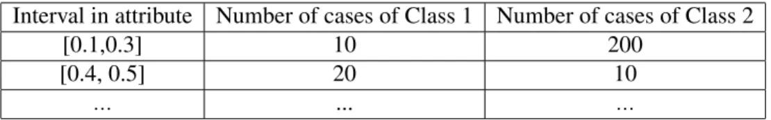
The first step of the algorithm is producing the dominance classifier structure. This structure is essentially a table containing intervals{V}as well as the number of instances of each class in the interval. In the example in Table 5 whereX1, X2, ..., Xi, ..., Xnaren
predictor attributes, which form n-D space, the interval [0.1,0.3] on the predictor attribute
Xicontains 10 cases of class 1 and 200 cases of class 2, while the interval [0.4, 0.5] on
the sameXicontains 20 cases of class 1 and 10 cases of class 2.
TABLE 5: Example Intervals of Distribution of Cases of Classes in an Attribute Interval in attribute Number of cases of Class 1 Number of cases of Class 2
[0.1,0.3] 10 200
[0.4, 0.5] 20 10
... ... ...
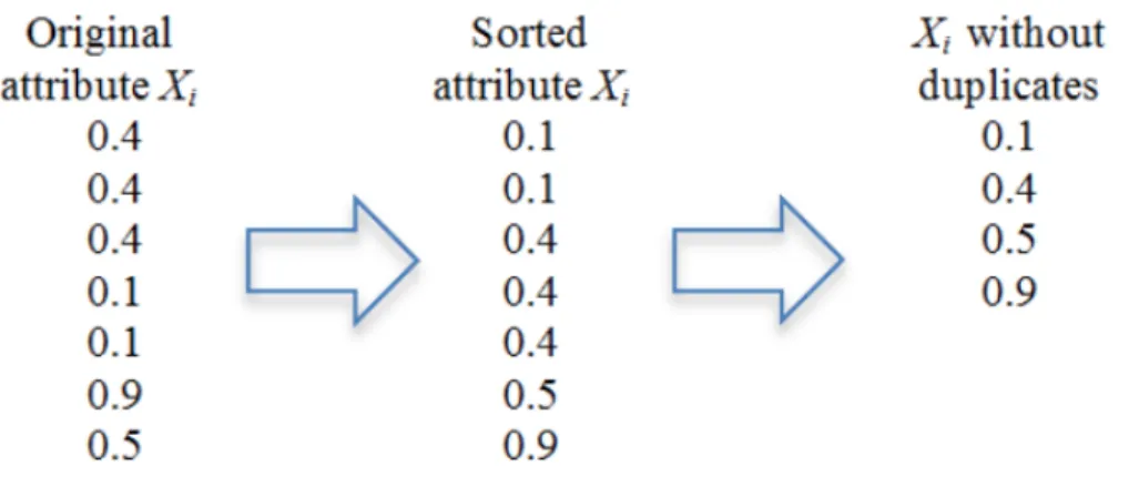
Step 1.1sort values on predictor attributeXiby ascending value, then remove all
FIGURE 1: Sorting and Removing Duplicate Values Described in Step 1.1.
Step 1.2computing the number of times each value appears by class for each predictor attribute. Figure 2 illustrates this step.
FIGURE 2: Class Quantities of Predictor Attribute Values Described in Step 1.2.
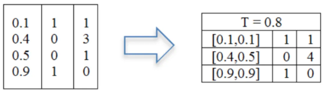
Step 1.3use the data obtained from each predictor attribute in steps 1.1 and 1.2 to calculate the dominant class for each point, i.e. the class with the greatest number of cases relative to all other classes. After obtaining the dominant class of each point, group them all into intervals that are contiguous, dominated by the same class, and have a size greater than or equal to some threshold, T (see Grid Search). Figure 3 illustrates this step.
FIGURE 3: DCP Classifier Constructed from Class Quantities and Predictor Attribute Values Described in Step 1.3.
Pseudo Code for DCP
Algorithm 1 contains the pseudo code for the base DCP algorithm capable of constructing the classifier, as has been described in the previous sections.
Algorithm 1DCP Pseudo code
1: procedureDCP(data, n, t ) .
2: data normalize(data) .Normalize attributes, 0 to 1
3: i 0; 4: whilei < ndo 5: attribute getAttribute(data, i) 6: sorted ascendingSort(attribute) .(1.1) 7: set removeDuplicates(sorted) .(1.1) 8: consolidated ConsolidateByClass(set) .(1.2)
9: consolidated ConsolidateByV alue(consolidated) .(1.3)
10: intervals JoinRatiosGreaterT hanT(consolidated, t) .(1.3)
11: i+ +
12: end while
13: end procedure
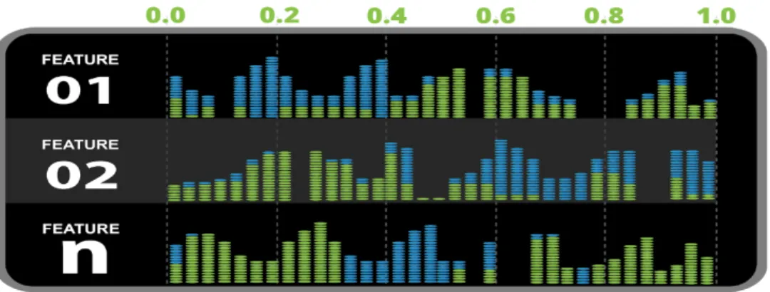
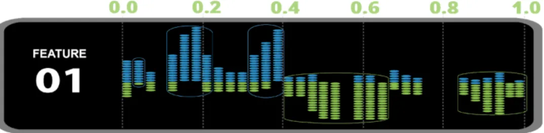
number of points for a given class to the total number of points of all classes. In this case, class 1 is represented by green values, and class 2 by blue values.
FIGURE 4: Example Features’ Class Dominance.
In Figure 5 an additional visualization technique is used on a single attribute to further accentuate the nature of DCP’s dominance intervals. Instead of aligning the values to the bottom as in Figure 4, values are instead aligned to the middle by class, then stacked outward in a descending fashion for class 1 and ascending fashion for class 2. Note, this step is not a required part of building the DCP classifier, however may offer additional insights for those wishing to understand DCP on a more intuitive level.
FIGURE 5: Example Values Centered to Enhance Visualization of Dominance
Next, Figure 6 shows a visual simulation of the selection process for dominance intervals of a given attribute. Intervals are selected with respect to a given threshold, T, which can most simply be described as the minimum dominance ratio required for a
dominance interval to be added into the classifier. Grid search (described later on) is used to obtain the value 0.8 for T, resulting in the retention of several intervals (denoted by the boxes), colored according to the dominate class.
FIGURE 6: Example Values Selected by Dominance Threshold
Looking at Figure 7, we can see all of the values from Figure 6 that did not fall within a dominance interval were removed. This empty space represents the areas for which no usable training data was provided, and for which no prediction is possible. In proximity to these empty spaces, the dominance intervals which were represented by colored outlines in Figure 6, have been replaced by single boxes colored according to dominate class. By constructing the visualization in this way, it is possible to illustrate exactly which values will predict which class.
FIGURE 7: Classifier for a Single Attribute.
FIGURE 8: Example Voting Classifier for N Attributes.
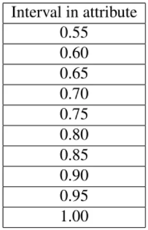
Finding the Dominance Threshold via Grid Search
The dominance threshold, T, is defined as the ratio of total number of points for class j to the total number of points of all classes. To determine the value of T for each attribute, DCP implements a grid search within a given range of values. Next, DCP constructs a classifier for each. After creating the classifier tests will be run via the training data to determine the most accurate value. The classifier associated with the most accurate value will be kept to be used in the final classifier, while the others will be discarded.
As can be seen in Table 6, the number of grid searches for each attribute is defined by the domain expert providing the hyperparameter. The domain expert will determine
TABLE 6: Example Search Space Using Grid Search at a Value of 0.05. Interval in attribute 0.55 0.60 0.65 0.70 0.75 0.80 0.85 0.90 0.95 1.00
the granularity of T between each grid in the search space, which will then be divided into equal parts starting from the minimum to the maximum possible dominance threshold, i.e. 0.5T1.0.
Feature Dependency and Assumption of Independence
Dissimilar to NB, which may or may not treat all features as statistically
independent, DCP does not use dependencies between features, but rather ignores them.
Interpretation of Discontinuous Intervals
Whether discrete or continuous, single or in multiples, dominance intervals work in the same way for each attribute of all classes, due to DCP’s characteristically non-overlapping topology. In other words, whether attributes are continuous or discrete, the actual training data always contains a finite number of n-D points. These points are processes by DCP, as described in the prior DCP steps. As far as discrete attributes
overlapping of actual cases is concerned, the case will go though one of the values. From a visualization perspective, tiny lines can be used to represent stand out intervals such as [6,6] which we can make wider by actually visualizing [1,1] as [1,2), [2,2] as [2,3) and so on with [6,6] as [6,7).
The Unbalanced Scenario
In the case which there exists an unbalanced class size relative to the size of the opposing class, consistent with supervised learning convention, the best option is likely going back to the original training data and oversampling the minority class or under-sampling the majority [26] until a more desirable balance is achieved, i.e a stratified k-fold cross validation.
Classification Rules to Classify Cases
This part of the algorithm starts fromStep 2.1and computes the dominant class in each attribute for a given casex, wherex = (x1, x2, ..., xi, ..., xn)and is an n-D point in
the n-D space ofX1, X2, . . . , Xn. As stated previously, the dominance level is defined as
the ratio of the total number of points for a single class to the total number of points of all classes. For a given point, a search is then conducted to determine if there exists an interval containing the point in the attributeXi.
If such an interval exists, the subsequent attributes are referenced to calculate the dominant class in said interval. If such an interval does not exist then no prediction is associated with the given attribute. For example, in a positive case, having valuexi= 0.2,
the algorithm finds interval [0.1,0.3], and then seeing that class 1 is represented by 10 samples, and class 2 is represented by 100 samples, class 2 being the greater of the two this interval would be used for class prediction for attributeXi.
Step 2.2: After determining which class is dominant for the givenx=
(x1,x2,. . .,xn) for eachxion the respective attributeXi, the algorithm uses a voting
method to combine dominance values, based on individual attributes, to determine the total prediction. For example, for the input n-D point x, withxi = 0.25, the use of Table
3 would activate interval [0.1,0.3], which in turn would predict class 2 over class 1 due to dominance on this interval with a much greater number of instances of class 2. For thisx, class 2 is the most dominant class onXiand interval [0.1, 0.3] is the dominant
interval onXi. Thus from such a table, a simple test of the valuexican determine the
corresponding interval V used in the prediction of the class of n-D points.xis based on
the most dominant classjin this interval for the given attributeXiwith a simple one
attribute prediction ruleR0:
If x= (x1, x2, ..., xi, ..., xn) & xi2V & hj =max(h1(V), h2(V), ..., hk(V))
thenx 2 class j
where(h1(V), h2(V), ..., hk(V))are the numbers of cases of classes 1,2,. . .,k,
respectively, that have values in intervalV on attributeXi.
The ruleR0is based on a single attribute, while we have n attributes. We will use the notationj(x, i)to denote that class j is a dominant class for the n-D casexbased on
the attributeXi. Next, we will formulate rules that take into account all n attributes where
each dominant classd(x, i)gets some vote value. Below we consider four voting methods (1)
that differ in the number of votes assigned to each dominant class.
Each dominant interval gets one vote, Vij = 1, if j is a dominant class on Xi, else Vij = 0
in a simple base method for n attributes, that we denote as VM1. In VM1 the total vote for classjis a sum of votes for this classVij for all attributesXi, it is the number of
times whend(x, i) =jby considering all attributesXi, V(j)=Pn
i=1Vij =|d(x, i) =j, i= 1, n|}
The classification decision is based on the comparison of total votes and finding their max value,
V(t)(x) =max(V(1)(x), V(2)(x), ..., V(k)(x)) with theclassification ruleR1:
IfV(t)(x) =max(V(1)(x), V(2)(x), ..., V(k)(x)), thenxbelongs to classt
Thus, the voting method, VM1, is resulted in formula (4). For each class j it checks that a given dimension’s valuexiwas classified to that classj(belongs to the interval that
is dominated by classj), and if so, adds a single class-vote to classjvotes, then find the
max of these sums in formula (4). This method is problematic for many datasets, because it assumes that all attributes are equally predictive. In VM1 intervals containing a larger number of cases are equally predictive (or equally negligible) as intervals with fewer values, e.g., intervals with 4 points and 100 points when both dominated by the same class. Here we have an underrepresented interval for the class with only 4 points.
Other voting methods. For sake of brevity, the other more complex voting methods denoted VM2-VM4 assign votesVij andV(1)(x), V(2)(x), ..., V(k)(x)will be summarized
as follows:
(2)
(3)
VM2: attempts to correct for the reliance on underrepresented intervals
VM3: attempts to find the middle between high-accuracy intervals being underrepresented and single intervals being overrepresented
VM4: limits the number of votes any single attribute is allowed to cast to a maximum amount, and via another threshold, by placing lower bounds on interval sizes allowed to vote
Visualization of the DCP Algorithm
Figure 9 illustrates the visualization of the structure of the WBC dataset. Here each vertical block represents a single dimensionXiof the this cancer dataset with
the values normalized to be the interval [0,1]. The blue represents dominant intervals where majority attribute values belong to benign cases, the red represents intervals where majority attribute values belong to malignant cases, and the white color indicates absence of values in the training set. This dominance structure is constructed in steps 1.1-1.3 of the DCP algorithm and represents the first 9 partitions of the 10-fold cross validation. Each column contains a noticeably large area absent of any values. Moreover, the DCP algorithm will refuse to classify cases that have value in these intervals [27]. The single red and blue polylines visualize single 9-D point (case) as it is visualized in Parallel Coordinates [28], the height of the nodes of these polylines are valued with respect to attributesX1,X2,. . .,X9. These examples are drawn from validation sets formed by
10-fold cross validation processes using random selection, then are superimposed over the classification blocks to visualize exactly where the patient’s data are malignant-like, and benign-like. It is visible that the case in Figure 9 is mostly in the benign areas and the
FIGURE 9: Result of Randomly Selected Sample 1
FIGURE 10: Results of Randomly Selected Sample 2
The visual explanation is based on Figure 9. Consider the black polyline (case) in Figure 9, where it is visible that all its attributesX1-X9are in the dominant intervals of the blue class. These dominant intervals have direct meaning in the breast cancer domain because they are in the original breast cancer attributes. This alone allows domain experts
to make professional judgments on them. In Figure 10, the red case belongs to 7 red dominant intervals and only 2 blue dominant intervals, which allows direct professional judgments by domain experts.
Textual Explanation of the DCP Algorithm
The textual explanation in the following form accompanies this visual explanation: A [ dimension-name ] of [ value ] falls within the known interval [x,y], which consists of
n instances of class 1, and m instances of class 2. In Table 7 and Table 8 the first attribute is normalized to [0,1]: A normalized value of clump-thickness at 0.6 falls within the known interval [0.5, 0.7], which consists of 95 instances of class 1, and 5 instances of class 2.
TABLE 7: Tabular pro-con Explanation by Dominant Interval Supporting Class 1. 0.33 0.11 0.00 0.00 0.11 0.00 0.11 0.00 0.00 0.22 0.11 0.00 0.00 0.00 0.00 0.11 0.00 0.00 0.55 0.11 0.00 0.00 0.00 0.00 0.66 0.00 0.00 0.11 0.11 0.11 0.00 0.00 0.00 0.66 0.00 0.00 0.44 0.11 0.00 0.00 0.11 0.00 0.22 0.00 0.00 0.22 0.11 0.00 0.00 0.11 0.11 0.22 0.00 0.00 0.33 0.11 0.00 0.00 0.11 0.11 0.22 0.00 0.00 0.00 0.11 0.11 0.00 0.11 0.00 0.11 0.00 0.00
TABLE 8: Tabular pro-con Explanation by Dominant Interval Supporting Class 2. 0.44 0.11 0.22 0.33 0.11 0.66 0.22 0.55 0.00
0.77 0.11 0.33 0.00 0.44 0.00 0.44 0.33 0.33
Table 2 formally shows this explanation with some pro cases on the WBC attributeX2.
Figure 11 visualizes one of the cases that support class 1. In this way, visual and tabular explanations complement each other.
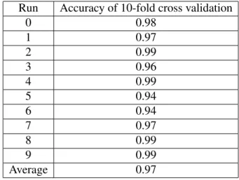
Accuracy of the DCP Algorithm
The WBC dataset was obtained from the University of California at Irvine machine learning repository [29] and used in these experiments. WBC consists of 688 samples, and 9 features, each normalized on a [0,1] interval. The features are: clump thickness (F1), uniformity of cell size (F2), uniformity of cell shape (F3), marginal adhesion (F4), single epithelial cell size (F5), bare nucleoi (F6), bland chromatin (F7), normal nuclei (F8), and mitoses (F9). Table 2 shows, in detail, classification accuracies using 10-fold cross validation with DCP’s voting method. As can be seen from the table, the first run achieved the highest classification accuracy of 98.5% with average accuracy of 97.01%.
TABLE 9: Detailed ten-fold Cross Validation Results with VM4 Run Accuracy of 10-fold cross validation
0 0.98 1 0.97 2 0.99 3 0.96 4 0.99 5 0.94 6 0.94 7 0.97 8 0.99 9 0.99 Average 0.97
Comparison of DCP with Interpretable Models
Understanding the results obtained by DCP can be aided by looking at the most current accuracies obtained by other interpretable non-intepretable machine learning models alike.
First, Looking at the literature concerned with interpretable machine learning models we see that the C4.5 J4 decision tree generating algorithm, and fuzzy decision trees offer a good point of comparison for their state-of-the-art accuracy (for interpretable models) and for their similarity with regard to using the same WBC dataset, and 10-fold cross validation. On the same data, the highest average accuracy obtained by the DT models was reported to be 94.82% [30, 31, 15, 25], whereas accuracy obtained by DCP is 97.01%, the highest of any known interpretable method. Comparing DTs to DCP by their average accuracy, we can see that DCP has some advantages with respect to accuracy, however, it is not to say that these two algorithms are intrinsically similar, as there are notable differences.
Using DCP, for example, we can see that if out of n attributes, just one attribute exists with pure intervals (intervals that contain cases of a single class each) then this attribute alone is sufficient to classify training data with 100% accuracy. This is also a condition for non-overlapping of two hyper-rectangles. All other attributes and respective hyper-rectangles of cases of classes in n-D will play the role of context. An attempt to eliminate all of them from consideration can produce classification errors on new data that have values of these attributes outside of the training data. An example can be found in the Iris data where a single attribute (petal size) allows full separation of class 1 (Setosa) and class 2 (Versicolor) [32, 33]. On the other hand, an adversarial example can be found
using ten times larger or smaller than values in the training data from a very different flower, or a completely artificial and non-existent object.
For the Decision Tree (DT) models, the presence of two pure intervals for two classes leads to a shortest possible decision tree with a single attribute and single split, i.e., a simple interpretable model,if Xi<T then class 1elseclass 2. Here T is any point
between two intervals, e.g., T=1.5 for intervals [0,1] and [2,3].
This simple case allows showing the difference between DCP and DT. DT
generalizes outside of the actual intervals [0.1] and [2.3] to the area between them (1,2), where the first half of its point are classified to class 1 and the other half to class 2, when
T = 1.5.
The justification for T=1.5 as opposed to any other value from (1,2) is nontrivial, if possible. Moreover, any T from (1,2) can produce an overgeneralization with an erroneous classification of cases between intervals, (similar to the Iris example) by classifying non-existent cases. Moreover, The same difference takes place in the
situations without pure intervals, but with multiple dominant intervals. Another important difference is the voting process is not present in DT explicitly, where instead all solutions are propositional statements and potentially overgeneralize, for instance:
Ifx1 >5 &x2<8 &x3 >4thenx= (x1, x2, x3)2class1
For example if we letx= (x1, x2, x3)andx12 [6,8],x22[4,5], andx3 2[5,9], in this situation DCP provides richer and more specific interpretable information than DT on the same data via intervals such asx= (x1, x2, x3)2class1, because:
x1 = 5 2 [3,6]onX1where class 1 dominates class 2 with ratio 10/1 & and this interval covers 75% of all class 1 training cases
x2 = 4.5 2 [4,5]onX2where class 1 dominates class 2 with ratio 6/1 and this interval covers 90% of all class 1 training cases
x3 = 7 2[5,9]onX3where class 1 dominates class 2 with ratio 4/1 & this interval covers 65% of all class 1 training cases.
As we see, the DCP explanation can show the size and representativeness of each dominance interval used. For example, this could allow a given domain expert to judge how marginal a given position of a new case x is in the interval, and how well the training data are represented in the dominant intervals.
The base voting in DCP is conceptually equivalent to constructing a disjunctive normal form (DNF). LetP(xi)be a property ofxithat is behind the vote for x withxifor
class 1. i.e., IfP(xi) =true, then voteV(xi) = 1.
Consider a case of voting that 2 out 3 attributes votes for class 1 forx = (x1, x2, x3). This voting is equivalent to the following DNF,
if[P(x1) & P(x2)or (P(x1) &P(x3) & (P(x2) &P(x3)], then x2class 1 Similarly, a DNF can be constructed for a larger number of attributes, e.g., 7 out 10 attributes vote for class 1. The long DNF is hard to discover and understand, but it is easier to communicate with domain experts as a voting statement.
Another difference between DTs and DCP is that DT rules are sequential, starting from the attribute at the root of the tree, while DCP is invariant to the order of attributes. A consequence of this is that follow-up splits in the DT (space), which depend on previous splits, can allow for new rules to be discovered that might otherwise not have been discovered with DCP. On the other hand, by covering a lesser number of cases in the process, DTs could possibly yield under-representative models. Moreover, DTs tend to suffer from overfitting, particularly when training reduces local error at the expense of generalization.
Non-interpretable Models
Comparing the accuracies achieved by DCP those obtained using non-interpretable machine learning models such as Support Vector Machines (SVMs) and Artificial Neural Networks (ANNs) proves possible the ability to create machine learning algorithms that are both interpretable and at least as accurate non-interpretable methods.
Using the same WBC dataset with 10-fold cross validation, the best accuracy reported for SVM in [34] is 96.995%. Furthermore, others such as the combining of SVM, C4.5, Decision Trees, Naive Bayesian classifiers, and k-Nearest Neighbors algorithms, achieved accuracies as high as 96.84% [35] and 96.99% [29]. Additionally, different versions of less interpretable methods such as SVM and ANN produced more accurate results that range from 97.97% to 99.51% on the same 10–fold cross validation [25].
The average accuracy of 97.01% obtained by the DCP algorithm is higher than accuracies of interpretable methods reported in [30, 31, 15, 25] that are in the interval [94.36, 95.27] which has an average of 94.82, however is still below than accuracies of non-interpretable methods in the interval [97.97, 99.52] averaging 98.74. Our 97.01% differs from the average for interpretable models by 2.19% and by 1.73% from non-interpretable models. Thus, while the DCP algorithm did not reach the accuracy of the non- interpretable methods (SVM and ANN), its classification model does however offer interpretability and the highest level of accuracy obtained for all known interpretable models on the WBC data.
CHAPTER IV
REVERSE PREDICTION PATTERN RECOGNITION
Reverse Prediction Pattern Recognition (RPPR)
Reverse Prediction Pattern Recognition (RPPR) is a boosting algorithm which augments DCP by discovering pair relations between attributes, learning from said relations, and then overriding inaccurate DCP predictions to increase overall accuracy. To simplify, DCP finds patterns in the form of dominant intervals in individual attributes, and then RPPR finds patterns in pairs-of-attributes that are specific to DCP false-positive or DCP false-negative cases. After learning these pairs —though hypothetically n-tuples could be used —in training, our experiments show that interpretable models can be as accurate as many state-of-the-art ”black-box” neural networks like ANN and SVM.
Reverse Prediction Pattern Recognition (RPPR) Basis Schema
The basis schema of the RPPR algorithm consists of the following steps:
(1)Present elements of DCP algorithm as Boolean vectors
(2)Find training cases misclassified by the DCP algorithms,
(3)Discover all unique pairs for DCP False-Negative (FN) and DCP False-Positive (FP) n-D points on training data
(4)Finding FN and FP n-D points in the validation dataset with these unique pairs
Outline of RPPR’s Five Steps
Step 1
The first step of presenting elements of DCP algorithm as Boolean vectors is as follows. Consider if we let n-D training dataset with attributesX1,X2,. . .,Xn. Let V1,V2,. . .,Vnbe the dominance intervals for class 1 found by the DCP algorithm on these
training data. Then, we produce n Boolean attributesB1,B2,. . .,Bnand n-D Boolean
point b=(b1,b2,. . .,bn) in these attributes from n-D point x=(x1,x2,. . .,xn) as follows: bi = 1xiVi, i.e.,xibelonging to the dominance interval of class 1 on attributeUi. See
Figure 11 for an example of this with several 5-D Boolean points.
FIGURE 11: Binary n-d Points Produced from DCP Algorithm
Step 2
Figure 14 illustrates the second step of finding training cases misclassified by the DCP algorithm.
Step 3
The third step of finding unique pairs for DCP negative and DCP false-positive n-D points is to:
(3.1)Make a second pass on the training data, and compare the DCP predicted value to the Target value;
(3.2)Collect all pair-combinations (bi,bj) for false-positive n-D points in the array
A, denoted as bin-A, all pair-combinations (bi,bj) for false-negative n-D points in the
array B, denoted as bin-B, all pair-combinations (bi,bj) for true-positive n-D points in
array C, denoted as bin-C, and all pair-combinations (bi,bj) of true-negative n-D points in
the array D, denoted as bin-D;
(3.3)Remove all pair-combinations from bin-A which also exist in bin-C;
(3.4)Remove all pair-combinations from bin-B, which also exist in bin-D.
Step 4
all pairs fromb5, starting from the pair (b1,b2)=(1,0) on the top and ending with the pair
(b4,b5)=(0,1) on the bottom. We call pairs in this set candidate-pairs. Notice n-D pointb5 is a DCP false-negative n-D point, therefore we are looking for the pairs (xi,xj) that can
be used to alter the DCP prediction (0) forb5.
Green lines connect (bi,bj) pairs on the left, which are solely present in DCP
false-negative n-D pointsb1-b5, to uniquely false-negative n-D points. These pairs are also shown on the right in Figure 14. The remaining pairs that present in both false-positive and true-positive n-D points are marked by the grey lines connecting them to respective non false-positive n-D points.
Step 5
The process of discovering unique pairs is repeated for allbi. After pair discovery,
a set of all unique pairs is assembled to be used in step (5) where these unique pairs are used to recognize and reverse false predictions made by DCP.
In this way, the RPPR algorithm produces unique pairs for DCP false-negative n-D points, found on training data, and in a similar process, the unique pairs for false-positive n-D points. Followed by step (4), these unique pairs used to find FN and FP n-D points in the validation set, and then reverse them on the step (5). It is however worth noting the possibility that the training data is too small —not enough n-D points to reverse DCP false prediction —which would result in undefined behavior the RPPR algorithm. The good news is that remedying this situation requires nothing more than an increase in the amount of training data, if possible.
RPPR Results
Using DCP boosted with RPPR, accuracies ranging from 97 to 100% have been achieved, averaging 99.3% using 10-fold cross validation, exceeding other known
published results. Unlike SVM and other non-interpretable methods, DCP & RPPR offers clear, visualizable, and fully explainable results which domain experts require in verticals characteristic of high cost errors (necessitating model explanation).
Algorithmic Boosting
Boosting methods demonstrated their efficiency in many tasks [32, 29]. In adaptive boosting (AdaBoost) meta- algorithm and related methods, the boosted classifier is a linear combination of the weak classifiers [32] of the form:
C(xi) =↵1h1(xi) +↵2h2(xi) +...+↵mhm(xi).
Boosting, thus, is a form of linear regression. The booster learner’s job in the two-class two-classification task [20] is to find weak hypotheses ht:X ! { 1,1}and boosted
classifierC(xi)the output final hypothesis:
H(xi) =sign(C(xi)).
Boosting commonly assumes that weak classifiers are classifiers of the same type such as decision trees. While decision trees are interpretable, the interpretation of the boostedC(xi)andH(xi)is more difficult, especially if the number of voting trees is
large.
To avoid this difficulty, RPPR does not create a weighed-sum of weak classifiers of a given type, but instead builds a classifier of another type on top of the DCP classifier,
RPPR Boosting
Similarities to other boosting approaches can be found in RPPR’s shared focus on improving the performance of its existing classifiers, of which centers on the cases poorly classified by DCP. Typically, other boosting approaches first assign equal weight values (1/n) to each case for computing the total prediction error, then attribute lesser weights to cases with inaccurate predictions. Afterward, these cases are then carried over for retraining the classifier on subsequent boosting iterations forcing it to learn the cases that in which it failed on in previous iterations.
RPPR Weighting
As far weighting is concerned, RPPR sets up only two weights: 0 for cases
correctly classified by the DCP algorithm, and 1 to cases that were incorrectly classified. Furthermore, RPPR is trained to improve accuracy on the later cases of false predictions ensuring that the accuracy on former cases will not deteriorate later by RPPR, overcoming a major drawback boosting methods have long held.
An Additional point worth noting is how RPPR operates at a more fine-grained resolution by considering the interactions between attributes within each case, instead of prioritizing each misclassified case entirely. Doing so has resulted in RPPR being Computationally more efficient, as only a single pass on the training set is needed instead of successive rounds.
In conclusion, RPPR does indeed boost DCP classification accuracy up to the level of many state-of-the-art black-box models, it does so in a very different way to that of AdaBoost and other similar boosting methods, maintaining strict interpretability. In our experiments on the benchmark WDBC data, interpretable algorithms have reached the level of accuracy of non-interpretable algorithms.
CHAPTER V
MULTIPLE DISK FORMAT
Multiple Disk Format (MDF)
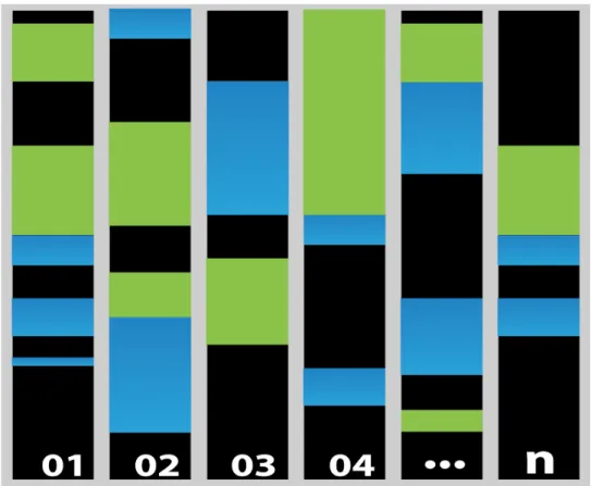
Multiple Disk Format (MDF) can provide a method to more clearly visualize data encoded as a set of binary values{0,1}, especially where each record belongs to one of two classes that are themselves encoded as 0 or 1 [36], such as DCP. In Figure 16 we use MDF to help visualize the relationships between Boolean vectors created by DCP during classification as follows. MDF containsn+ 1layers called disks, wherenis the number of attributes in a given dataset. Together these disks represent all n-D Boolean vectors, i.e.2ntotal vectors. The first disk (disk 0) contains a single zero-vector, i.e. each
value in the vector is zero, diskncontains a single vector with all1, and diskkcontains all n-D points that havek“1” (Hamming norm is equal tok). In each disk, the Boolean
vectors are positioned according to the location of non-zero values in descending order, i.e. decreasing in value from left to right. For example in a 3 attribute dataset, the bottom disk would contain the value 000; the second row from the bottom would contain the values 100,010,001; the third row from the bottom would contain the values 110,101,011; and the fourth (top) row would contain the value 111.
Visualizing 512 9-D Boolean Vectors - DCP
Figure 16 shows MDF representing all 512 9-D Boolean vectors. Here each cell in the top 5 disks have more 1’s than 0’s and each cell in the bottom 5 disks has more 0’s
cells blue. Similarly, actual DCP Boolean vectors with more 0’s than 1’s are located in the bottom 5 discs, where DCP classifs them to class 1. Correct DCP classifications are represented by the cells colored blue, and incorrect are colored red. In this way, MDF shows all misclassified cases as 10 blue cells (bars) in the five top discs and 3 red cells in the five bottom disks.
FIGURE 14: Multiple Disc Format
Visualizing 512 9-D Boolean Vectors - RPPR
Keep in mind that while MDF excels at showing where values are misclassified, it does not show how common a given misclassified binary vector may be. For this reason, such as is the case with DCP, rarely occurring misclassified cases may have a disproportionate presence in the visualization compared to the data. For example, looking at the top half of Figure 16 we see there are 10 misclassified (blue) binary vectors, and in the bottom half there are 3 misclassified (red) vectors, amounting to 13 out of 98 classified binary vectors, or 87%, whereas the actual classification accuracy obtained by DCP on the data was over 97% as previously noted. In addition, the original MDF does
not account for the possibility of the occurrence of a given binary vector in both cases. To rectify the latter of these issues a modified MDF was created, shown in Figure 17.
Modified MDF for RPPR
FIGURE 15: Modified Multiple Disc Format
The modified MDF (M2DF) is particularly illustrative in the case of DCP due to the binarization of DCP class attributes used in conjunction with voting. In MDF all classes that would produce a DCP vote for class 1 are at the bottom and all that would produce a vote for class 2 are at the top. In doing so, the problem of occlusion and overlapping-data that are characteristic of most other visualization methods is mostly avoided. An exception is the special case occurs when the same Boolean vector occurs in both classes. In such cases, a modified MDF may be used to prevent any loss of information, and maybe constructed by splitting the cell which maps to both classes by the ratio of the number of instances of one class to the other. For example, if the Boolean vector a has 90
Modified MDF After RPPR
FIGURE 16: Modified Multiple Disc Format After RPPR
Looking at data presented in MDF format, we can easily distinguish between four scenarios. In the first scenario, each case is represented by a single Boolean vector, belongs to a single class, and is indeed classified accurately by DCP. In the second scenario, each case is represented by a single Boolean vector, belongs to a single class, and is misclassified by DCP. The third scenario consists of each case being represented by a single Boolean vector, occurring in both classes, and will be classified with an accuracy proportional to the ratio in which the presence of one class is dominant over the other (favoring the more dominant of the two). In the fourth scenario, a given binary was not found to belong to class 1 or class 2.
The first scenario represents where DCP classifies and predicts successfully, obtaining accuracies of around 95% of all cases on the WDBC dataset. The second scenario, where a binary vector votes one class yet belongs to only the opposing class, represents the cases where RPPR can learn the pairs associated with said misclassifications and then flip them to the correct class, boosting DCP’s accuracy by
between 3 to 5 percent. The third scenario represents a potential for future work where a given vector that was binarized by DCP and appears in both classes, could then be reexamined via deeper analysis to find subtle differences between the two which could boost classification in much the same way RPPR does.
CHAPTER VI
CONCLUSION
Over the course of this thesis, significant time and energy have been applied to researching the development of interpretable models capable of competing with black-box models such as ANNs and SVMs, often highly accurate. A list of accomplishments during this time includes: the development of two new accurate and fully interpretable algorithms, a human-friendly visual explanation for these new interpretable models, and traditional textual explanations that can be provided via natural language or mathematical forms. In addition, the multidimensional visualization technique MDF, although not original to this thesis, was applied to DCP and RPPR in a novel ways, resulting in the newer MDF2 algorithm capable of visualizing class changes occurring on behalf of RPPR.
The two algorithms developed over the course of this research, DCP and RPPR, have each achieved significant milestones. DCP has achieved, on several benchmark datasets, the highest known accuracy of any interpretable ML models on these data. RPPR took the success of DCP further, via a novel boosting method, creating the only known process by which competitive glass-box models can be constructed to successfully match, or exceed, the accuracy of black-box models such as ANNs and SVM, without sacrificing interpretability. Furthermore, we also have strengthened our results via reported more successful experiments in [37].
In addition to my contributions to this work, Dr. Kovalerchuk has also played an invaluable role, making significant contributions. I developed ideas of both DCP and RPPR algorithms, implemented them and conducted computational experiments and comparisons. I also implemented MDF algorithm developed by Dr. Kovalerchuk for the
use with DCP and RPPR algorithms on the benchmark WBC data. I was guided in the development of this work by Dr. Kovalerchuk on all these stages. During this process he formulated the problems to solve, suggested how to formalize and formulate these algorithms and their improvements, suggested datasets for the experiments, and advised me on ways to conduct experiments and compare results.
The door has been opened to the development of ML models which are both fully interpretable and as accurate as black box models. Although our research saw many milestones achieved, there is still much more work to be done before such algorithms are battle ready. Ideas for future work include further testing on more diverse datasets, increasing the number of DCP classes from 2 to n, and increasing RPPR pairs to n-tuples.
REFERENCES CITED
[1] A. Sachan, “Convolutional neural networks comparison based on accuracy,” 2019. [2] W. Knight, “The dark secret at the heart of ai,” 2019.
[3] A. Arnx, “Neural network explained for beginners,” 2019. [4] Y. Bulatov, “The root cause of slow neural net training,” 2019.
[5] N. Cristianini and B. Scholkopf, “Support vector machines and kernel methods the new generation of learning machines,” inAi Magazine 23.3, pp. 31–31, 2002.
[6] H. Drucker, D. Wu, and V. N. Vapnik, “Support vector machines for spam categorization,”IEEE Transactions on Neural networks, vol. 10, no. 5, pp. 1048–1054, 1999.
[7] K. Dhiraj, “Advantages and disadvantages of decision trees,” 2019.
[8] J. Su and H. Zhang, “A fast decision tree learning algorithm,” inAAAI, vol. 6, pp. 500–505, 2006.
[9] J. Valente, “Decision tree from scratch in python,” 2019.
[10] G. Seif, “Guide to decision trees for machine learning and data science,” 2019. [11] V. Krakovna, “Building interpretable models: From bayesian networks to neural
networks,” 2019.
[12] G. Chauhan, “All about naive bayes,” 2019.
[13] DARPA, “Explainable artificial intelligence,” inDARPA-BAA-16-53, 2016.
[14] Z. Lipton, “The mythos of model interpretability,” inCommunications of the ACM, pp. 1–28, 2018.
[15] D. Chaki and A. Das, “A comparison of three discrete methods for classification of heart disease data,” inBangladesh Journal of Scientific and Industrial Research 50.4, pp. 293–296, 2015.
[16] H. Lakkaraju, S. Bach, and J. Leskovec, “Interpretable decision sets: A joint framework for description and prediction,” inProceedings of the 22nd ACM SIGKDD International Conference on Knowledge Discovery and Data Mining, pp. 1675–1684, 2016.
[18] A. Abdel-Zaher and A. Eldeib, “Breast cancer classification using deep belief networks,” inExpert Systems with Applications Volume 42, Issue 10, pp. 139–144, MAICS, 2016.
[19] A. Bhardwaj and A. Tiwari, “Breast cancer diagnosis using genetically optimized neural networks,” inExpert Systems with Applications 42.100, pp. 4611–4620, MAICS, 2015.
[20] G. Cooper, V. Abraham, C. Aliferis, and J. Aronis, “Predicting dire outcomes of patients with community acquired pneumonia,” inJournal of Biomedical Informatics, pp. 347–366, 2005.
[21] G. Cooper, B. Buchanan, C. Aliferis, and J. Aronis, “An evaluation of machine learning methods for predicting pneumonia mortality,” inArtificial intelligence in medicine 9.2, pp. 107–138, 1997.
[22] R. Caruana, Y. Lou, J. Gehrke, P. Koch, and M. Sturm, “Intelligible models for healthcare: Predicting pneumonia risk and hospital 30-day readmission,” inIn Proceedings of the 21th ACM SIGKDD international conference on knowledge discovery and data mining, pp. 1721–1730, 2015.
[23] Parliament and C. of the European Union, “General data protection regulation, article 22,” inGeneral Data Protection Regulation, 2016.
[24] B. Kovalerchuk and E. Vityaev,Data mining in finance: advances in relational and hybrid methods, vol. 547. Springer Science & Business Media, 2006.
[25] Y. Freund, R. Schapire, and N. Abe, “A short introduction to boosting,”
Journal-Japanese Society For Artificial Intelligence, vol. 14, no. 771-780, p. 1612, 1999.
[26] Educba, “What is the naive bayes algorithm,” 2019.
[27] B. Kovalerchuk and N. Neuhaus, “Toward efficient automation of interpretable machine learning,” in2018 IEEE International Conference on Big Data (Big Data), pp. 4940–4947, IEEE, 2018.
[28] B. Kovalerchuk and V. Grishin, “Adjustable general line coordinates for visual knowledge discovery in nd data,”Information Visualization, vol. 18, no. 1, pp. 3–32, 2019.
[30] F. P. Pach and J. Abonyi, “Association rule and decision tree based methods for fuzzy rule base generation,”World Academy of Science, Engineering and Technology, vol. 13, pp. 45–50, 2006.
[31] J. R. Quinlan, “Improved use of continuous attributes in c4. 5,”Journal of artificial intelligence research, vol. 4, pp. 77–90, 1996.
[32] B. Kovalerchuk and E. Vityaev, “Visual knowledge discovery and machine learning,” inData mining in finance: advances in relational and hybrid methods. Vol. 547. Springer Science Business Media, 2006.
[33] B. Kovalerchuk and V. Grishin, “Reversible data visualization to support machine learning,” inInternational Conference on Human Interface and the Management of Information, pp. 45–59, Springer, 2018.
[34] G. Salama and M. Abd-elghany, “Breast cancer diagnosis on three different datasets using multi-classifiers,”Breast Cancer (WDBC), vol. 32, no. 569, p. 2, 2012. [35] S. Aruna, S. Rajagopalan, and L. Nandakishore, “Knowledge based analysis of
various statistical tools in detecting breast cancer,”Computer Science & Information Technology, vol. 2, no. 2011, pp. 37–45, 2011.
[36] B. Kovalerchuk, F. Delizy, L. Riggs, and E. Vityaev, “Visual data mining and discovery with binarized vectors,” inData Mining: Foundations and Intelligent Paradigms, pp. 135–156, Springer, 2012.
[37] N. Neuhaus and B. Kovalerchuk, “Interpretable machine learning with boosting by boolean algorithm,” in2019 Joint 8th International Conference on Informatics, Electronics & Vision (ICIEV) and 2019 3rd International Conference on Imaging, Vision & Pattern Recognition (icIVPR), pp. 307–311, IEEE, 2019.
APPENDIX
GITHUB SOURCE FILES