Improving local corrections for the radar vertical reflectivity profile using the linear depolarisation ratio

(1)

UNIVERSITY OF READING

Department of Meteorology

Improving local corrections for

the radar vertical reflectivity

profile using the linear

depolarisation ratio

Caroline Georgina Sandford

A thesis submitted for the degree of Doctor of Philosophy

July 2018

(2)

Declaration

I confirm that this is my own work and the use of all material from other sources has been properly and fully acknowledged.

Caroline Georgina Sandford

Acknowledgements

I would like to thank my supervisors Anthony Illingworth, Robert Thompson and Dawn Harrison for their creativity, patience and support throughout this PhD. I am very grate-ful to Malcolm Kitchen for his expertise and engagement with this project, which were a great source of encouragement to me. I would also like to thank Donal Adams from the Met Office radar hardware team, for his input on the radar network upgrades and reflectivity calibration scheme; and Nawal Husnoo, for his unfailingly prompt responses and invaluable insights during the writing of this thesis.

(3)

Abstract

A major source of errors in radar-derived quantitative precipitation estimates (QPEs) is the vertical reflectivity profile (VPR). A feature of particular importance is the radar “bright band”: a reflectivity enhancement due to the melting of large snowflakes that occurs in the majority of high latitude rainfall, and which if misrepresented can cause order of magnitude errors in surface QPEs. Recent upgrades of several national weather radar networks to dual polarisation provide opportunities to refine the identification of bright band in operational radar measurements, and to improve subsequent determination and corrections for VPR.

This thesis applies information from the linear depolarisation ratio (LDR) to improve classification of VPRs at the pixel scale. Using a unique dataset of high resolution vertical profiles, values of LDR in the melting layer are shown to provide a seven-fold increase in probability of detection of non-bright band reflectivity profiles over the current UK operational criterion. In the context of the Met Office local VPR correction scheme, an LDR-based classification step alone is shown to produce improvements in bias and RMSE of more than 1 mm h−1 for high rain rates in non-bright band conditions. The high resolution vertical profile dataset is then further used to improve the param-eterisation of VPR shapes for correction at the local scale. Using a simulation method adapted from previous literature, three possible non-bright band VPR shapes are de-fined and their performance objectively compared to a control (no correction) profile. The most skilful profile is applied to a high intensity non-bright band case study in com-bination with LDR-based VPR classification, yielding further improvements to QPE bias and RMSE. Improvements to the stratiform profile are also investigated. The conclusions of this thesis indirectly support the use of local over global VPR corrections to maximise the accuracy of radar QPEs at the sub-kilometre scale.

(4)

Introduction

1.1 Background

The use of radar for monitoring and quantification of meteorological phenomena has become globally established over the past several decades. The term “radar”, originally an acronym RADAR, stands for “radio detection and ranging”, and dates from the use of radio frequency installations for military surveillance in the 1940s. Since then the details of radar hardware and frequency have diversified, and have come to fulfil a range of operational and research functions within the meteorological community.

The Met Office weather radar network began its development in 1976 with the installation of a 5.4 GHz (5.6 cm wavelength) Plessey radar at Hameldon Hill, in Lancashire (Kitchen and Illingworth, 2011). The initial aim of the installation was to monitor real time rainfall to inform preparations to mitigate flood impacts, such as occurred in 1952-1953 in the South and West of England. By 1985 the network had expanded to four radars, to 12 within the next decade, and currently stands at 15. UK radar products now also incorporate data from two non-Met Office radars in Ireland and one in the Channel Islands.

In the 33 years since the official launch of the network in 1985, substantial developments have been made both to the science of rainfall estimation, and to the uses of radar anal-yses. Algorithms to identify and remove non-meteorological echoes, and processing of meteorological artefacts such as the radar bright band (section 1.5.3), have led to steadily increasing reliability and corresponding demands on the accuracy of radar precipitation estimates. Met Office radar products are currently used by operational meteorologists to inform and advise, and by the Met Office / Environment Agency collaborative Flood Forecasting Centre in high impact situations. Rain rate composites are also assimilated into the Met Office numerical weather prediction (NWP) model via a latent heat nudging

(9)

scheme (described in Jones and Macpherson, 1997), as well as providing a strong com-ponent of the Short Term Ensemble Prediction System (STEPS) rainfall extrapolation nowcast (Bowler et al., 2006). As well as their scientific applications, real time radar products are highly visible to the general public, through publication on the external website and availability as part of the Met Office mobile app.

Radar quantitative precipitation estimates (QPEs) suffer from substantial uncertainties from a range of different sources (Villarini and Krajewski, 2010). Common problems in rainfall estimation include remote sensing issues, such as attenuation and contamina-tion from non-meteorological echoes, as well as more complex inaccuracies arising from the microphysical relationships between the radar measurement and liquid water con-tent. For hydrological users, these errors can have significant detrimental impacts to downstream products, such as runoff, pluvial and fluvial flood forecasting (Berne and Krajewski, 2013). The impacts are severe enough that some modellers prefer to ingest point rain gauge accumulations instead of a gridded radar product, despite the benefits in spatial coverage and grid representativity that radar provides. There is therefore strong motivation for continuing research and development towards improving the accuracy of radar QPEs.

With the proliferation of radar networks around the world over recent decades, radar sys-tems have also undergone significant developments. One of the most important of these breakthroughs has been the introduction of dual polarisation: the ability to transmit and receive independently in the horizontal and vertical polarisations. This technology pro-vides the capability to measure the shape of hydrometeors rather than their size, which allows more complex inferences to be made as to the type and quantity of precipitation falling at any given time.

While research into the uses of dual polarisation data has been active since the mid-1970s, over the past 10-15 years dual polarisation hardware has developed to a high enough quality and reliability to be used operationally. This has prompted many national meteorological services to upgrade their radar networks to dual polarisation capability (eg Kumjian, 2013; Figueras I Ventura and Tabary, 2013; Helmert et al., 2014; Gabella et al., 2016). The recent culmination of several upgrade projects has shifted the focus of dual polarisation research into the operational sphere, prompting the development of a range of algorithms for real time radar quality control, corrections and QPE.

The UK national radar network, including the Channel Islands radar, has recently under-gone a complete upgrade to dual polarisation. The Met Office Weather Radar Network Renewal project (WRNR), which began in 2011 and was completed in December 2017, replaced and rennovated existing hardware at these 16 UK radars (but not the two in Ireland). The new radars were designed and built in-house using commercial off-the-shelf components (Darlington et al., 2004, 2016), and are capable of high quality dual

(10)

polarisation measurements comparable to those of leading research facilities (appendix A). This upgrade, combined with the quality of the new data available, provides unique opportunities for research and development in the context of the UK climate and existing radar processing algorithms.

This thesis investigates improvements to radar rainfall estimation in the UK through the use of a specific dual polarisation parameter, the linear depolarisation ratio (LDR), to inform corrections for the vertical profile of radar reflectivity (VPR). Understanding the variability in radar-measured reflectivity with height, and how this compares to intrinsic reflectivity at the surface, is a crucial step in obtaining accurate QPEs (section 1.5). In this introductory chapter the principles of meteorological radar are described, from the initial measurement to the estimation of surface rain rates. The nature of the radar measurement and its meteorological interpretation are covered in section 1.2, followed by an overview of operational networks and scan strategies in section 1.3. Section 1.4 introduces the concept of dual polarisation, which in recent years has become the new standard for operational radar networks. The sequence of processes by which UK radar reflectivities are converted into rainfall estimates, including determination and correction for the VPR, is described in section 1.5. Having established this context, the full aims and an outline of this thesis are presented in section 1.6.

1.2 Principles of meteorological radar

Weather radar works on the principle of echo location. A transmitter first sends out a pulse of electromagnetic energy, followed by a passive phase in which the receiver “lis-tens” for echoes. These microwave pulses are transmitted via a parabolic antenna whose properties determine the radar beam pattern and gain. In “receive” mode the antenna assembly acts in reverse: power returning is focused into the antenna and measured by the receiver. Radar receivers must be robust in detecting power returns across the 8-9 orders of magnitude spanned by meteorological echoes, and must also be extremely sen-sitive, given the significantly decreased power of reflected echoes in comparison to the transmitted pulse. A physical “T/R” switch operates to transition the radar between “transmit” and “receive” modes, which protects the receiver assembly from the higher energy transmission.

1.2.1 Rayleigh scattering, reflectivity and the radar equation

The basic meteorological measurement derived by weather radar is known as “reflectiv-ity”. This is calculated directly from the received power, and is a function of properties of meteorological targets within the radar pulse volume.

(11)

The power received at the radar from a population of hydrometeors is given by: pr= AP σi r2 (1.1) A= ptg 2_λ2_Θ2_l 1024π2_ln(2) (1.2)

Hereptis transmitted power,g is the antenna gain,lthe pulse length,λthe wavelength,

and Θ the angular beam width; which makesAa constant for a given radar (Bringi and Chandrasekar, 2001). These fixed beam properties are discussed in section 1.3.2. Variable factors in this equation are range from the radar, r, and the scattering cross-section of each hydrometeor,σi.

The scattering cross-section of a radar target depends on both the size of the target and the radar wavelength, which determines the scattering regime. The wavelength of meterological radars is chosen so that the hydrometeors of interest are around an order of magnitude smaller than the incident wavelength, and are therefore sampled within the Rayleigh regime. In this regime, the electromagnetic pulse E~i transmitted by the radar

induces an oscillating dipole in the target hydrometeors, and the associated movement of electrons generates its own fieldE~s, which is scattered both forward and backward along

the transmission path. The amplitude of the backscattered field from a dielectric sphere relates to properties of the incident radiation and the target as:

~ Es = k2₀ 4πr m2−1 m2_{+ 2}×4πD 3 ~ Ei (1.3)

wherek0 is the wavenumber of the incident radiation (which is inversely proportional to

its wavelengthλ),mis the complex refractive index andDis the diameter of the spherical target (Bringi and Chandrasekar, 2001, equations 1.32a and b). The backscattered power (∝ ~ Es 2

) from a point target in the Rayleigh regime is therefore proportional toλ−4and the sixth power of the target diameterD6.

Following from equation 1.3, the scattering cross-section of a Rayleigh point target is defined as:

σi=

π5|κ|2_D6

i

λ4 (1.4)

where dielectric factorκ relates to the complex refractive indexm as:

|κ|= m2−1 m2_{+ 2} (1.5) Radar reflectivity, which is the sum of diameters to the sixth power, can then be defined in terms of the sum of scattering cross-sections from hydrometeorsiof different diameters

(12)

per unit volume: Z=XD6_i = λ 4 π5_|_κ_|2 X σi (1.6)

The definition of reflectivity as a sum of diameters is valid only for liquid rain drops with sphere-equivalent diametersDi; however the definition in terms of scattering cross

section is general. Combining equations 1.1 and 1.6 leads trivially to the radar equation:

Z=Cprr2. The conversion from power to reflectivity is typically performed at the radar

site, using the precalculated radar constantC and the range r calculated from the echo arrival time.

The relationship between reflectivity and the volume of water sampled by a radar pulse (through theD6 term) depends on the dielectric factorκ, which varies with precipitation phase. Reflectivity (equation 1.6) is defined with respect to the value for liquid water:

|κw|2 = 0.93. However dielectric factor values for frozen hydrometeor species are

signif-icantly lower, varying in proportion to snow density up to a maximum of |κi|2 = 0.176

for solid ice (Sauvageot, 1992, chapter 2, pg 97-98). This means that the reflectivity of snow is at least 5 times lower than the reflectivity of the equivalent volume of liquid rain drops, which impacts the drop diameters and water volume that can be inferred from a reflectivity measurement. The behaviour of κ and its impact on radar reflectivities is discussed in more detail in section 2.2.2.

For meteorological purposes reflectivity is usually expressed as an integral rather than a sum. Defining the drop size distribution N(D)dD as the number of hydrometeors per unit volume with diameters betweenDand D+ dDyields the most widely used form of the definition:

Z =|κw|−2

Z ∞

0

N(D)|κ|2D6dD (1.7) This linearZ is in units of mm6m−3, with Din mm and N(D) in mm−1m−3.

Given that meteorological reflectivities span several orders of magnitude, reflectivity val-ues are often given in logarithmic dBZ units:

ZdBZ = 10log(Z) (1.8)

Reflectivities in rain typically fall within the range 18-55 dBZ, with reflectivities greater than 55 dBZ often indicating the presence of hail in convective situations (Bringi and Chandrasekar, 2001).

1.2.2 Reflectivity and rain rate

The main function of meteorological radar in an operational environment is to provide real time estimates of rain rate at the ground surface. Rain rate R is the volume of

(13)

liquid water reaching the ground per unit time, and like reflectivity (equation 1.7) can be defined in terms of an integral over rain drops of different diameter:

R= π 6

Z ∞

0

N(D)vt(D)D3dD (1.9)

where vt is the terminal fall velocity of each drop. The fall velocity is generally

ap-proximated by a power law vt(D) = αDβ, where β lies in the range 0.6-0.67 for liquid

rain drops (Bringi and Chandrasekar, 2001). Radar rain rates are usually expressed in millimetres per hour (mm h−1).

The relationship between reflectivity and rain rate (ZR relation) depends on the form of the drop size distribution. Marshall and Palmer (1948) use a rain rate dependent expo-nential to describe a measured drop size distribution. The slope of this expoexpo-nential can be expressed as a function of the median drop diameter,D0 (Bringi and Chandrasekar,

2001), so that: N(D) =N0exp −3.67D D0 ≡N0e−x (1.10)

Assuming a rain drop fall velocity proportional toD0.67, it follows that:

Z ∝ Z ∞ 0 N0D6exp −3.67D D0 dD∝N0D70 Z ∞ 0 x6e−xdx (1.11) R ∝ Z ∞ 0 N0D3.67exp −3.67 D D0 dD∝N0D04.67 Z ∞ 0 x3.67e−xdx (1.12) Z ∝N₀(1−7/4.67)R7/4.67≈N₀−0.5R1.5 (1.13) This specific example illustrates the more general form of the ZR relation, which is expressed as a power law:

Z =aRb (1.14)

whereais inversely proportional to the square root of the intercept parameter N0. Such

fixed ZR relationships are used throughout the operational community to estimate rain rates from radar networks.

In realityN(D) is not always exponential, nor isN0 a constant, but varies with rain type

and climatology. Optimal coefficients for equation 1.14 can be determined empirically, using disdrometer or other independent measurements in conjunction with radar. These methods typically find the exponentbin the range 1.4-1.6, but estimates ofavary much more widely due to its dependence on drop concentration (Battan, 1973). The form suggested by Marshall and Palmer (1948) for stratiform precipitation is Z = 220R1.6, which is frequently approximated asZ = 200R1.6 (the “Marshall-Palmer relation”).

(14)

1.3 Operational radar configurations

1.3.1 Scanning meteorological radar

Figure 1.1: Example of a reflectivity PPI at 0.5o elevation from the Channel Islands radar, 14:59 UTC on 28th May 2018. Maximum range of 255 km.

Operational radars collect the majority of their data in scanning mode. For scan-ning meteorological radar the antenna ro-tates in azimuth while transmitting and receiving, building up a circular “plan po-sition indicator” (PPI) image of targets surrounding the radar (eg figure 1.1). A PPI scan is typically taken at a fixed non-zero elevation angle above the horizon-tal, and has a maximum range of between 60 and 300 km. Due to Earth curvature and the refractive properties of the atmo-sphere, the height of the radar beam above the ground increases with range according to the four-thirds Earth approximation:

H =Hrad+

p

r2₊_R02_{+ 2}_rR0_sin_θ _(1.15)

whereR0 = 4

3RE and RE = 6374 km (Earth radius) (1.16) where Hrad is the antenna height, r the range (in km) from the radar, and θ the scan

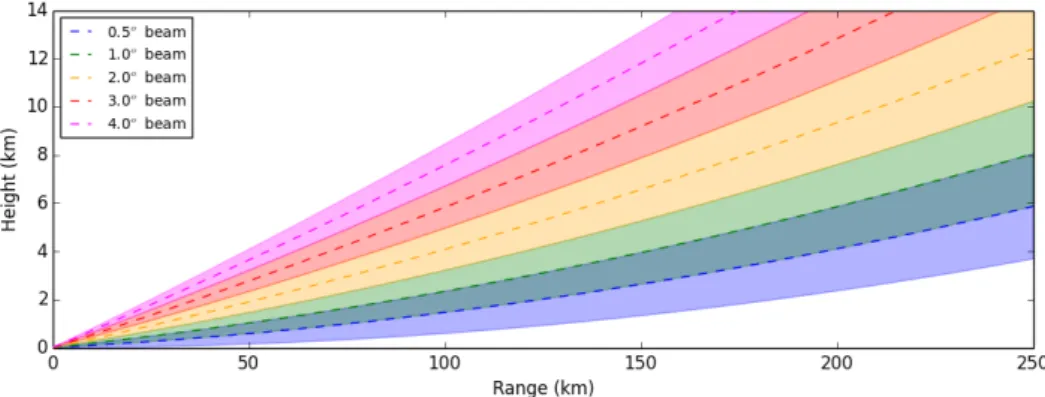
elevation angle (Doviak and Zrni´c, 1993). This means for example that at a range of 250 km, a radar PPI measurement at 0.5oelevation would be centred around 6 km above the ground (figure 1.2). The radar beam also broadens with range, with a typical operational beam width of 1o (eg Harrison et al., 2012; Figueras I Ventura and Tabary, 2013; Helmert et al., 2014; Koistinen and Pohjola, 2014) spanning an azimuthal and vertical distance of 1 km at 50 km range, 2 km at 100 km, and more than 5 km at the maximum 255 km range of the Met Office radars (as illustrated in figure 1.2).

Operational weather radars typically operate a scan strategy including several PPIs at different elevations above the horizontal. Radar “volumes”, consisting of a series of PPIs taken within a fixed time period, are repeated at frequencies of 5 to 15 minutes depending on the update frequency required of radar precipitation estimates. The use of volumes provides additional vertical coverage in PPI scan mode, and allows higher elevation scans to be used to replace lower elevation data contaminated by non-meteorological echoes (section 1.5.1). Radar volumes can also be used to generate 3D products such as hy-drometeor type, for vertical reflectivity profile estimation, and for the construction of 2D

(15)

Figure 1.2: Schematic showing beam heights and broadening of the five PPI elevations used in the Met Office QPE scan strategy.

gridded products at fixed altitudes (constant altitude PPIs, or CAPPIs).

The five beam QPE scan strategy used by Met Office radars is shown in figure 1.2. This is a compromise well suited to the precipitation systems most frequently observed in the UK. In lower latitude climates where convective systems can reach greater depths, and at centres where volume reflectivities may be used in numerical weather prediction (NWP), higher elevation scans may also be included. There is a trade-off between including more scans to observe the whole precipitation column and completing the radar volume scan within the time available.

1.3.2 Properties of the radar beam

The spatial resolution of a radar and the limits of its sensitivity to precipitation depend on properties of the hardware and the radar beam. The radar constantC, which relates the radar reflectivity to the received power, is influenced by several factors including the wavelengthλ, pulse length l, and the angular width of the beam Θ.

Wavelength and dish diameter

To maximise both sensitivity and spatial resolution (in azimuth), it is desirable for the power transmitted by a radar to be focused into a narrow beam. Assuming a Gaussian beam power profile, the half power beam width Θhpachieved by a given radar is a function

of the ratio between the radar wavelengthλand the diameter of the parabolic reflector dishdA:

Θhp=

1.27λ dA

(1.17) where Θhp in radians is twice the off-axis angle at which the radar beam power reduces

(16)

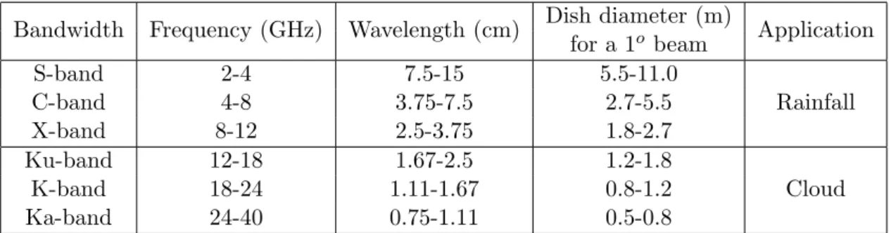
Bandwidth Frequency (GHz) Wavelength (cm) Dish diameter (m) Application for a 1o beam S-band 2-4 7.5-15 5.5-11.0 Rainfall C-band 4-8 3.75-7.5 2.7-5.5 X-band 8-12 2.5-3.75 1.8-2.7 Ku-band 12-18 1.67-2.5 1.2-1.8 Cloud K-band 18-24 1.11-1.67 0.8-1.2 Ka-band 24-40 0.75-1.11 0.5-0.8

Table 1.1: The main frequency bandwidths used by rainfall (S-X) and cloud (Ku-Ka) radars, for operational and research applications.

Operational weather radars within the UK and Europe typically operate with an angular beam width of around 1o (eg Kitchen et al., 1994; Tabary, 2007), which provides the kilometre-scale spatial resolution with which rainfall estimates have historically been required by the modelling and verification communities. The main radar wavelength bands used for this purpose are listed in table 1.1. A 1o beam width at a C-band wavelength of 5.3 cm (as used by the UK radar network) requires a parabolic reflector dish 3.86 m in diameter. At S-band, due to the longer wavelength, a 7-8 m dish is required. Conversely at X-band, this spatial resolution can be achieved with a dish 2 m in diameter. For these reasons, X-band radars are a popular choice for field studies, as higher spatial resolution can be achieved with a smaller and more portable instrument. Longer wavelengths tend to be chosen for ground based operational radars, due to the wider spatial coverage and lower sensitivity to meteorological attenuation (section 1.5.2).

Pulse length, averaging and pulse repetition frequency

Each pulse transmitted by a weather radar has a durationT, which relates to the spatial pulse length l by the speed of light (l =cT). The shorter the pulse duration, the finer the radial resolution of the radar image. For two targets along the same azimuth to be resolved, the end of the transmitted pulse must reach the first target before the start of the echo from the second target arrives back at the first. The minimum target separation at which this is possible defines the spatial resolution, which is equal to half of the spatial pulse length.

Shorter pulse length also allows for a higher pulse repetition frequency (PRF), defined as the number of pulses transmitted per second (in Hz). A higher sampling rate can reduce the error on derived reflectivities. However, since an echo can only be attributed with certainty to a given pulse if it is received before the next pulse is transmitted, a higher PRF reduces the maximum unambiguous range of the radar. Given a time between successive pulse initiations (in seconds) ofτ = 1/PRF, the maximum unambiguous range iscτ /2.

(17)

The reflectivities returned from a radar site are not calculated from a single pulse, but from the average received power pr from several transmitted pulses. The phase of the

echo from a meteorological target is random, meaning that the standard deviation of the pulse-to-pulse power received from a target is equal to the mean power, assuming that the pulses are independent. Averaging overM independent pulses reduces the standard deviation on the derived measurement by a factor of√M, which improves the accuracy of the measurement.

The number of independent pulses is not the same as the total number of pulses aver-aged to calculate reflectivity, due to the temporal correlation between successive mea-surements. The correlation between pulses separated by lagm varies with wavelengthλ

and PRF: ρ(m, τ) = exp − 4πmσvτ λ (1.18)

whereσv is the velocity spectrum width (Doviak and Zrni´c, 1993). This can be used to

calculate the number of independent pulses M contributing to the average of a larger, correlated sampleMt.

For Met Office radars, standard QPE reflectivity measurements are collected at a PRF of 300 Hz with a spatial pulse length of 300 m. Two radial bins are averaged for each measurement, meaning that the data are returned at a radial resolution of 600 m. Given an azimuthal resolution of 1o and a scan rotation rate of 8.4os−1, this means that each reflectivity measurement is calculated using the average power fromMt= 37 pulses. With

a Doppler spectrum width of 1 m s−1 this is equivalent to roughly M = 16 independent pulses, or a four-fold reduction in noise on the averaged reflectivity measurement. The PRF of 300 Hz corresponds to a maximum unambiguous range of 500 km; but due to the height of the beam (equation 1.15) only reflectivities within 255 km of the radar are used operationally.

1.3.3 Radar networks

For monitoring rainfall on a national level, most meteorological services operate a net-work of radars to maximise spatial coverage and service reliability. Data from these networks are typically combined to synthesise a “composite” product, which is composed of maximum, highest quality, or weighted average rain rate estimates from all contribut-ing radars. The number of radars in a network is related to land area: the smallest European networks consist of only two or three radars, with networks of 15 to 20 radars being typical of the larger European nations.

(18)

Figure 1.3: Status of the UK national radar network after completion of the Weather Radar Network Renewal project (WRNR). Different shading (dark to light) indicates coverage within 50 and 100 km respectively of the nearest radar.

from two more in Ireland and one in the Channel Islands (figure 1.3). This network provides multiple coverage of most land areas, increasing the resilience of the network to outages and maintenance schedules. The Met Office QPE composite is generated using the highest quality rain rate estimate at each point, taking account of both geometrical factors (range and height of the measurement) and meteorological conditions. The 1 km gridded rain rate composite underpins the majority of downstream applications in the UK.

1.4 Dual polarisation radar

Section 1.2 introduced the general relationships between rainfall rate, reflectivity, and raw received power for meteorological radar. A simple reflectivity measurement for rain rate estimation can be made using a microwave pulse transmitted in any polarisation. However, developments in radar hardware over the past several decades have made it possible to transmit and receive power independently in two orthogonal polarisation

(19)

channels. Dual polarisation parameters, derived by comparing both the power and rela-tive phase of the polarised returns, can provide significant additional information on the properties of meteorological echoes.

1.4.1 Dual polarisation transmission modes

Most modern dual polarisation systems operate using a linear polarisation basis with horizontal (H) and vertical (V) channels. The preferred method for operational radars is to transmit equal power simultaneously in both the H and V channels: a 45o polarised or slant elliptical transmission. This is referred to in the literature as “SHV mode” or “hybrid transmission”. In addition to reflectivity (usuallyZh), the following SHV mode

dual polarisation parameters can be calculated:

• Differential reflectivity (ZDR)

• Copolar correlation coefficient (ρhv)

• Differential phase shift (Φdp)

The information provided by dual polarisation parameters, in general, relates to the shape of hydrometeors or other reflectors in the radar pulse volume. Section 1.4.2 gives an overview of the dual polarisation parameters listed above, with definitions and a brief description of the information they contain. This information is included for context, and is not used further in this thesis. The main focus for this thesis is section 1.4.3, which describes in detail the measurement and interpretation of the linear depolarisation ratio.

1.4.2 Interpretation and applications of SHV mode parameters

Differential reflectivity

Differential reflectivity is defined as:

ZDR = 10log Zh Zv (1.19) whereZh and Zv are the reflectivities calculated respectively from the H and V received

power. For meteorological echoes, ZDR provides a measure of the average axis ratio.

For liquid drops axis ratio is linked to diameter, with larger diameters producing more oblate spheroids. This means that ZDR can be used in combination with reflectivity Zh

to estimate parameters of the drop size distributionN(D) (Brandes et al., 2004), which in turn determine the optimal ZR coefficients for rainfall estimation (section 1.2.2). This is discussed further in section 1.5.4.

(20)

Since the axis ratio of rain drops is known to increase with increasing size,ZDR

measure-ments in rain should increase monotonically with reflectivity Zh. Meteorological values

ofZDR range from close to zero for light rainfall (low Zh), to up to 2 dB for very heavy

rain (highZh), and can be in excess of 4 dB for wet hail and melting ice, where liquid

water forms a torus around the melting particle that increases its axis ratio (Rasmussen and Heymsfield, 1987). ZDR responds to axis ratio differently for rain and snow, due to

the difference in dielectric factor. A rain drop with an axis ratio of 2 would have a very highZDR of 6 dB; but a dry ice pellet or graupel with the same axis ratio has ZDR of

2-3 dB, and a dry snowflake hasZDR of less than 1 dB (Doviak and Zrni´c, 1993). High

reflectivities colocated with regions of near-zeroZDRcorrespond to tumbling hail or

grau-pel, where hydrometeors are irregular but the average axis ratio due to non-preferential orientation is equal to 1.

It is possible for measured ZDR to be lower than expected behind strong reflectivity

echoes. This is due to “differential attenuation”, usually through heavy rain, where the horizontal component of the radar pulse is more strongly attenuated than the vertical. In extreme cases this can result in negative ZDR measurements, despite the positive or

neutral aspect ratio of hydrometeors in the radar pulse volume (eg figure 1.4b).

Copolar correlation coefficient

Radar parameters for a single range bin are not derived from a single pulse, but typically are averaged from up to 30 to 40 pulses (section 1.3.2). The relationship between power returns from individual pulses can be used to derive measures of signal variability in a sin-gle polarisation (eg the clutter indicator, section 1.5.1), as well as providing information as to the range of dual polarisation properties within the radar pulse volume.

The copolar correlation coefficient ρhv is the correlation between the Zh and Zv

time-series for separate pulses within the same range bin. The back-scattering matrix for a hydrometeor in the radar pulse volume is defined:

" Shh Shv Svh Svv # =ejδhh " |Shh| |Shv|ej(δhv−δhh) |Svh|ej(δvh−δhh) |Svv|ej(δvv−δhh) # (1.20)

whereδx elements describe the phase of the backscattered signal (relative to the incident

phase δhh) and the magnitude elements |Sx| are proportional to the square root of the

back-scattered power (and thus the square root of reflectivity) (Bringi and Chandrasekar, 2001). Using this notation,ρhv is defined:

ρhv=

|hShhSvv∗ i|

p

h|Shh|2ih|Svv|2i

(21)

The behaviour ofρhv is dependent on both the quality of polarisation separation and the

target hydrometeors. If the sampling volume contains a population of hydrometeors of similar size and shape, then the backscattered phase will tend to be consistent from pulse to pulse, so the correlation between timeseries will be high. These conditions are typical of rain. Where the quality of polarisation separation in the radar hardware is good,ρhv

measurements in rain are typically greater than 0.99.

Volumes containing a mixture of hydrometeor shapes and types give much less correlated returns. ρhv values of around 0.8 at low levels can indicate the presence of hail in heavy

convective rainfall. Melting snowflakes are also associated with a reduction in ρhv due

to their variety of axis ratios and canting angles. This property is often used to locate the melting layer in radar PPIs (eg Tabary et al., 2006; Boodoo et al., 2010; Giangrande et al., 2008; Kalogiros et al., 2013), the significance of which is introduced in section 1.5.3 and discussed in detail in chapter 2. ρhv can also be used to identify non-meteorological

echoes, which have correlation values typically below 0.5 with a distribution that is well-separated from that of precipitation.

Differential phase shift and specific differential phase

Differential phase shift (Φdp) measures the phase difference in degrees between echoes

returned in the H and V channels. The value of Φdp quantifies the difference in the

extent to which radar pulses are slowed by the change in refractive index (from air to precipitation) in the two polarisation channels.

The amount of phase shift is related to the amount of precipitation encountered, in terms of scattering cross-section. When a radar pulse passes through a region of oblate rain drops, the horizontal component is phase shifted more than the vertical component, which is defined as positive Φdp(eg figure 1.4d). Similar toZDR, drops with more oblate

shapes produce a higher positive Φdp. However unlike ZDR, Φdp is a difference not a

ratio, and is therefore also sensitive to the total drop concentration in the radar pulse volume.

Since Φdp is cumulative an additional useful parameter, “specific differential phase”

(KDP), can be defined as the gradient of Φdp along a radial. KDP in rain provides

an indirect measure of drop shape, but is also sensitive to the quantity of water in the radar pulse volume. This means that under certain conditions KDP can be used as an alternative to reflectivity in rainfall estimation (eg Brandes et al., 2003, see also section 1.5.4).

Φdp is a noisy measurement, with estimated random errors of at least ±3o even after

(22)

(a) (b)

(c) (d)

Figure 1.4: Example of different dual polarisation measurements from a rainfall event observed by the Channel Islands radar at 14:59 UTC on 28th May 2018. Top left: reflectivityZ (copied from figure 1.1); top right: differential reflectivityZDR; bottom left: ρhv; bottom right: Φdp.

these effects, Φdp values do not always increase monotonically with range. The noisiness

of the Φdp range profile means that it is not always possible to extract the underlying

monotonically increasing function, which means that accurate KDP values cannot be derived for every range gate or in all conditions. At the Met Office, KDP is calculated only in regions of rapidly increasing phase shift where the resulting value would be greater than 16o km−1 (corresponding to rain rates in excess of 10 mm h−1).

Combining parameters

In addition to their independent interpretation, the information provided by SHV mode parameters can be used in tandem to improve and extend beyond radar precipitation analyses. The main combined applications of dual polarisation are in the identification

(23)

of non-meteorological echoes and the classification of different hydrometeor types (eg Rico-Ramirez and Cluckie, 2008; Park et al., 2009; Wen et al., 2016). Classification of rain is based on the relationship betweenZh andZDR in regions of highρhv; while lower

correlations (0.8-0.9), high reflectivities, and zero or negativeZDR at low levels can

indi-cate the presence of hail. The melting layer in stratiform precipitation is identifiable by reducedρhv, high reflectivity and highZDR (eg Tabary et al., 2006). Non-meteorological

echoes can be identified by their rough “texture” (high spatial variability) in ZDR and

Φdp, and by very low correlation coefficients (Rico-Ramirez and Cluckie, 2008).

The dual polarisation characteristics of meteorological and non-meteorological echoes can be seen in the example in figure 1.4, which shows a rainfall event observed from the Channel Islands radar in May 2018. The rain in the radar image is characterised by high

ρhvand by smoothZDRandφdp, whereas regions of high reflectivity andρhvto the

North-West of the radar are identifiable as non-meteorological by their noisy signatures inZDR

andφdp. Areas of negativeZDR and highφdp to the South and East of the radar indicate

strong attenuation, which is consistent with the high reflectivities observed (panel (a)). The lower (≈0.9) values ofρhvin the region to the East of the radar suggest the presence

of strong convection and hail.

Although quality control can be applied throughout the radar domain, more quantitative applications of dual polarisation data, such as corrections for attenuation and rainfall estimation, are as yet limited to radar measurements in rain, where the preferential orientation of liquid drops leads to quantifiable relationships between drop shape and volume that provide useful additional information on liquid water content (Herzegh and Jameson, 1992).

1.4.3 Single polarisation transmission: the linear depolarisation ratio

In addition to simultaneous transmission, further information on drop properties can be derived from transmission in a single polarisation. The linear depolarisation ratio (LDR) is measured by transmitting plane polarised horizontal pulses and receiving in both polarisations. LDR is defined as the fraction of the plane polarised signal that is returned in the opposite polarisation:

LDR = 10log Zvh Zhh (1.22)

The mechanism by which a hydrometeorological target may depolarise the incident radar pulse is illustrated in figure 1.5. Figure 1.5a shows scattering from a horizontally oriented drop which does not depolarise. Figure 1.5b illustrates how when a drop is canted, the dipole induced along the major and minor axes generates a scattered electric field which

(24)

Figure 1.5: Depolarisation of a horizontally polarised incident radar pulse by a hydrometeorolog-ical target. Solid lines indicate the incident and scattered returns in the horizontal and verthydrometeorolog-ical polarisations, while dashed lines show how these resolve along the axes of the target hydrometeor. a) An oblate, horizontally oriented drop which does not depolarise. b) An oblate, canted drop which generates a small vertical component from the horizontally polarised transmission.

is not aligned with the incident polarisation. It is clear from this schematic that both aspect ratio and orientation contribute to LDR, with higher axis ratios causing more depolarisation for a given canting angle.

The unique advantage of LDR as a parameter is this responsiveness to the orientation of hydrometeors within the radar pulse volume (Illingworth, 2004). Rain and snow consist of populations of largely horizontally oriented particles, and are therefore not depolarising

Figure 1.6: LDR PPI at 0.5o _{elevation from the} Channel Islands radar at 14:58 UTC on 28th May 2018. The high, localised values to the East of the radar are consistent with hail.

(figure 1.5a). The depolarised component in this case is not identically zero, but is limited by the cross-polar isolation of the dual polarisation system, so that the min-imum LDR measured in light rain (where drops are near-spherical) is typically be-tween -30 and -40 dB. However in the melt-ing layer, the oscillations of large, partially melted snowflakes cause significant larisation (figure 1.5b). The sum of depo-larised reflectivity components across the range of canting angles generates a char-acteristic melting layer peak of around -18 dB in LDR PPIs (Smyth and Illingworth, 1998; Illingworth and Thompson, 2011).

Depolarisation is not unique to melting snowflakes. In convective conditions, tumbling wet hail and graupel also generate high values of LDR, due to their essentially random canting angle. Figure 1.6 shows the LDR scan through the event shown in figure 1.4. Low

(25)

LDR of around -35 dB to the South-East of the radar corresponds to areas of rain. High values to the East are consistent with the signatures of attenuation inZDR andφdp, and

support the interpretation of reducedρhv in this region as hail. The high and noisy LDR

field surrounding the radar at short range is attributable to non-meteorological echoes. LDR cannot be calculated from SHV mode measurements, nor other dual polarisation parameters from LDR mode data. Due to competition for time in an real time scan strategy, operational measurements of LDR are therefore uncommon. Unlike many com-mercial radar installations, Met Office radars are designed to allow the collection and interpretation of LDR mode data, in addition to the more typically collected SHV mode scans.

1.5 Quantitative precipitation estimation

The process of obtaining quantitative precipitation estimates (QPEs) from radar data varies between National Meteorological Services (NMSs), but broadly speaking can be described in four main stages. Initially, the raw reflectivity volumes are filtered to remove echoes from non-meteorological targets such as buildings, trees, and complex terrain. Measurements are then corrected for power loss effects, such as partial beam blockages and attenuation through heavy precipitation (section 1.5.2). This may be followed by an adjustment to account for the height of the beam above ground level. The final stage is the conversion of corrected reflectivities, and occasionally dual polarisation parameters, into estimates of precipitation rate at the ground.

This section gives an overview of the main QPE steps applied by the Met Office’s opera-tional radar data processing system (Radarnet). This provides a context for the work of this thesis, and a reference for the additional processing performed as part of the analyses of chapters 5-7. While a full review of different NMS’s processing steps is not provided, reference is made where relevant to the main types of dual polarisation algorithms used within the operational community.

1.5.1 Identifying and removing non-meteorological echoes

Although weather radar is designed to observe and quantify precipitation, in reality echoes can be received from any number of sources. Close to the radar, a beam transmit-ted at low elevation may intercept targets such as buildings, trees, or complex terrain. Such stationary non-meteorological targets are known as “ground clutter”. Ground clut-ter echoes are often associated with very high reflectivities (at least 40-50 dBZ), which if misidentified can cause extreme overestimation or misleading detections where no

(26)

precip-itation is present (“false alarms”). Strong echoes may also arise from airbourne targets, such as aircraft, which often cause contamination close to airports. Aircraft echoes are strong but extremely localised, tending to be restricted to one range bin across one or two radar azimuths. Weak distributed echoes may be caused by “biological clutter”: flocks of birds or swarming insects. These echoes tend to be detected only at the high sensitivities and relatively low sampling heights of measurements very close to the radar. As well as aircraft, ground and biological clutter, radars near the coast may receive ad-ditional returns from the sea surface. This “sea clutter” has very different characteristics from ground clutter, since the beam is scattered from liquid water, so the reflectivity values and “texture” can be very similar to that of a precipitation field. Coastal radars may also detect large container ships, which have similar properties to aircraft echoes. Finally, non-meteorological echoes can arise from the ground itself. Anomalous prop-agation, or “anaprop”, occurs in situations where the atmospheric refractivity profile differs from that expected from climatology. Equation 1.15 for beam height assumes a “standard atmosphere”: a climatological profile of temperature and relative humidity that defines refractivity and dictates the expected propagation of the radar beam. In reality, variations in these physical profiles can cause the beam to deviate from its ex-pected path. This is primarily an issue in “super-refraction” conditions, where the beam is deflected more towards the ground than would be expected from the four-thirds Earth model. In anaprop cases, radar echoes from the ground and sea surface can be incorrectly interpreted as meteorological echoes at some height in the atmosphere.

The identification of non-meteorological reflectivities in Radarnet is performed on a scan-by-scan basis using one of two different methods, depending on whether or not dual po-larisation parameters are available for that particular scan. Reasons for dual popo-larisation data being unavailable may be temporary, for example as a result of scheduled mainte-nance, or can be due to standing issues such as limited bandwidth or non-upgraded radar hardware. For these reasons Radarnet remains flexible to inputs from both single and dual polarisation scans.

For single polarisation data, a number of successive filters are applied to identify and remove non-meteorological signals. Echoes are classified hierarchically, starting with ground and biological clutter, “speckle” (strong echoes over a handful of radar pixels due to ships and aircraft), radio frequency interference, and anaprop. The single polarisation filters in Radarnet rely heavily on a “clutter indicator” (CI) measure of signal variability (Sugier et al., 2002). Since ground clutter is stationary, echoes from clutter fluctuate very little from pulse to pulse, whereas precipitation echoes are constantly fluctuating. The initial CI-based clutter filter is followed by filters based on satellite cloud masks and precipitation climatologies built up from individual radars (Harrison et al., 2000). Sea clutter, which is difficult to distinguish from precipitation, is masked using a fixed

(27)

“clutter map” for affected regions of the lowest elevation scans.

For dual polarisation data, a na¨ıve Bayesian classifier based on Rico-Ramirez and Cluckie (2008) is used to identify non-meteorological echoes. This includes parameters based on the copolar correlation coefficient (ρhv), textures of differential reflectivity (ZDR) and

differential phase shift (Φdp) (section 1.4.2), and clutter phase alignment (CPA) (Hubbert

et al., 2009), which replaces the clutter indicator. CPA is used throughout this thesis for quality control, and is described in more detail in chapter 3. The main benefits of the dual polarisation algorithm are in its ability to distinguish sea clutter from precipitation, retaining valid data which would have been removed by a fixed clutter map, and in retaining some low reflectivities associated with drizzle rather than misclassifying them as “noise”. This allows the upgraded radars’ high sensitivities to be fully exploited at short range.

1.5.2 Power loss corrections for blockage and attenuation

Once non-meteorological echoes have been identified and removed from the raw radar data, the remaining reflectivities must be corrected for power loss effects. Physical ob-structions such as complex terrain can block all or part of the radar beam, causing a reduction in transmitted power which must be accounted for in order to derive accurate meteorological properties from measurements at longer range.

In the Radarnet system, beam occlusions are mapped to the radar sampling volume using a high resolution digital terrain map and the standard beam propagation model (equation 1.15). Where partial beam blockages affect less than half of the radar beam the data are flagged “usable”, but a power correction is applied to the measured reflectivity as part of correction for the vertical reflectivity profile (section 1.5.3). If a blockage affects more than 50% of the beam the data are flagged as unusable. Single ray occlusions are interpolated from reflectivities in adjacent rays, but for larger occluded sectors, QPE data is taken from higher elevation scans.

“Attenuation” refers to the weakening of the transmitted signal propagating behind any target in proportion to the amount of backscattered power. This reduction in transmitted power means that the beam is less sensitive to precipitation at ranges beyond strong echoes. Attenuation at C-band can reduce the intensity of long range precipitation, but complete extinction of the radar beam is rare, and corrections are usually effective in improving the quality of the attenuated data.

Correction for attenuation is performed for both single and dual polarisation data from the Met Office network. The single polarisation method is iterative, based on the re-lationships between rain rate and attenuation derived by Hitschfeld and Bordan (1954)

(28)

and Gunn and East (1954), with:

AdB = 0.0044R1.17 (1.23)

for the two way attenuation AdB at each range gate. An estimate of attenuation from

the first non-clutter range gate is used to adjust the reflectivity at the next gate, before calculating the attenuation from that next gate, adjusting the next, and so on. Such iterative correction methods are known to be unstable, so the Met Office correction is capped operationally at a factor of 3 in linear reflectivity (approximately 5 dB).

The dual polarisation attenuation correction method follows a two step procedure us-ing reflectivity, Φdp and long range radiometric noise emissions (Thompson et al., 2011).

Although Φdp can be used directly in dual polarisation attenuation correction schemes

(Bringi et al., 1990), the coefficient of the A(Φdp) relationship has been found to vary

significantly with both weather and climatology (Carey et al., 2000; Park et al., 2005; Vulpiani et al., 2008). The Met Office method uses a combination of the iterative cal-culation, A(Φdp) with ana priori coefficient, and emissions to constrain the total path

integrated attenuation at each radar azimuth. The median of these three estimates dic-tates the most suitable coefficient of Φdp, which is then used to calculate and correct for

attenuation at each range gate. This method has been shown to reduce over-correction resulting from the instability of the iterative reflectivity-based correction, and to improve the performance over a fixed coefficientA(Φdp) relation (Husnoo et al., 2018, additional

details Husnoo 2017, personal communication).

1.5.3 Estimating reflectivities at ground level

Radar reflectivities corrected for attenuation and beam blockage can be assumed to give a reliable representation of the meteorological properties of the radar pulse volume at the measurement height. However, for QPE, the desired measurement is of rainfall at the ground. Chapter 2 presents a more detailed review of the microphysics underlying the vertical profile of reflectivity (VPR), and the literature pertaining to its classification and correction in radar PPIs. An introductory overview is provided in this section. The radar reflectivity measurement is influenced by both the diameterD and dielectric constant κ of hydrometeors within the radar pulse volume (equation 1.7). Changes in both of these parameters with phase, which is determined by temperature gradient in the lower atmosphere, mean that the atmospheric reflectivity varies significantly with height. This has particular impacts in areas sampled around or above the height of the 0o_{C isotherm (or “freezing level”).}

(29)

comprised of a mixture of ice and air inclusions. These aggregates are much larger than their liquid counterparts, and their|κ|2_{is at least a factor of 5 smaller than that of liquid}

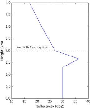
water (section 1.2.1). When these large, aerated snowflakes begin to melt, the accumula-tion of liquid water in and around the melting flakes causes a sudden increase inκ, and a correspondingly sharp increase in reflectivity of order 5-7 dB. As melting continues, the decreasing diameter and increasing terminal velocity of the target hydrometeors causes the reflectivity to fall again, reaching its final “rain” value typically a few hundred metres below the onset of melting (eg Kitchen, 1997; Kirstetter et al., 2013). This characteristic peak in reflectivity in the melting layer is known as the “radar bright band” (figure 1.7).

Figure 1.7: Example of the variation in reflec-tivity with height in a typical bright band case. The quantitative axes are for illustration only. Identifying the bright band in radar PPIs

is not straightforward. Figure 1.8 shows how the height and vertical extent of the radar beam increase with range. With in-creasing range the beam passes through rain, melting snow, snow and ice aggre-gates, and finally overshoots the precipi-tation top. The geometry of the measure-ment means that it is not possible to ob-serve variations in reflectivity with height directly with any degree of precision. Ad-ditional information is therefore needed in order to quantify and correct for the effects of bright band.

The bright band can pose significant prob-lems for radar QPE. If uncorrected, the en-hancement can cause severe (even order of magnitude) overestimation in surface

pre-cipitation estimates. Despite the conceptual simplicity of the bright band, however, in reality the details are extremely difficult to model, due to its strong dependence on the specifics of how each snowflake melts (see section 2.2 for a detailed review). Correcting for this vertical profile of reflectivity (VPR) is therefore extremely complex; and yet it is essential to obtaining accurate estimates of surface rain rate.

A large number of studies, both practical and theoretical, focus on situations such as those described above, where there is little vertical motion and the layers of frozen, melting and liquid precipitation are well separated. These conditions are described as “stratiform”. The Met Office corrects for stratiform VPR using a climatological profile shape, which is constrained using gridded NWP forecasts of 0oC isotherm height and satellite cloud top measurements. The idealised shape is fitted iteratively to the radar

(30)

Figure 1.8: Illustration of how and where the 0.5o_{elevation radar scan can sample liquid, melting} and frozen precipitation at different levels of the atmosphere. The height of the freezing level and precipitation top are for illustration only - in reality these have a range of values that vary spatially across the radar domain.

reflectivity measurement at each pixel using a known off-axis beam power profile (Kitchen et al., 1994; Kitchen, 1997). Bright band intensity is empirically related to rain-level reflectivity (Kitchen et al., 1994), and the integration over beam power is truncated to account for partial beam blockages in the vertical. A detailed discussion of this method and the associated profile shape is included in section 2.5.3.

An additional challenge to be overcome in correcting operationally for VPR is that differ-ent types of precipitation generate differdiffer-ently shaped profiles. In particular, “convective” situations characterised by strong vertical motion (Steiner et al., 1995) produce distinctly different profile shapes, which usually do not display a bright band (section 2.2.3). The shape of convective profiles is much more variable and difficult to constrain than the standard “stratiform bright band” (figure 1.7), and significantly fewer attempts have been made to develop convective corrections. As part of the Met Office VPR correction scheme, convection is diagnosed using a minimum reflectivity threshold 1 km above the 0oC isotherm. In these cases the reflectivity is assumed to be constant with height, and no VPR correction is applied.

1.5.4 Calculating surface rain rates

Having achieved a reflectivity estimate representative of surface conditions, the final conversion from reflectivity to rain rate can be applied. As discussed in section 1.2.2, the relationship between Z and R is not generally analytical, but can be approximated by a power law of the formZ =aRb. The coefficients of this power law are dependent on details of the drop size distribution.

(31)

It is not possible to measureN(D) in real time for operational rainfall estimation. Oper-ational ZR relations are usually climatological, using fixed coefficient values determined from previous studies. The Met Office uses the Marshall-Palmer relation Z = 200R1.6

(Marshall and Palmer, 1948), which performs well in the light to moderate stratiform rainfall responsible for the majority of precipitation in the UK.

For radar measurements in the rain layer, dual polarisation parameters can sometimes be used to improve QPEs. The ability to constrain the rain drop size distribution using

ZDR(section 1.4.2) is the principle underlying alternativeR(Z, ZDR) rain rate estimators.

Although such estimators arise frequently in the literature (eg Ryzhkov and Zrni´c, 1995; Zhang et al., 2001; Brandes et al., 2002, 2003; Ryzhkov et al., 2005), the requirements on ZDR calibration accuracy for QPE are stringent (±0.1 dB, Thompson (2007)), and

require a high quality system isolation not often achieved by operational radar networks (Hubbert et al., 2010).

In intense rainfall KDP can also provide an independent measurement of rain intensity (Brandes et al., 2003). The differential phase shift Φdp relates both to the average axis

ratio and the total water content along the radar beam propagation path (section 1.4.2), and its gradient provides an estimate of water content per km range. As the difference in phase shift between two channels, KDP has the significant advantage in heavy pre-cipitation of being less sensitive than reflectivity to attenuation. However, the inherent noisiness of the Φdpmeasurement means that KDP values are highly suspect at low

inten-sities. In the UK, KDP measurements greater than 16okm−1 (approximately 10 mm h−1 in rain rate) are used for rainfall estimation where the beam is below the melting layer, and have been shown to reduce QPE underestimation significantly at high intensities.

Dual polarisation rain rate estimators have been shown to deliver significant improve-ments the accuracy of QPEs calculated from rain level measureimprove-ments (eg Brandes et al., 2003). However in high latitude climates, and particularly in winter months, the ma-jority of the radar composite is derived from measurements at altitudes within or above the melting layer. For 0o_{C isotherm at 2 km, which represents an average for the UK}

climate (Kitchen et al., 1994), the domain in which the radar beam is fully within the rain extends only 60 km from the radar (figure 1.8). In conditions such as these, reflectivities in and above the bright band remain a vital source of QPE information, ensuring the continued relevance of research into improving corrections for the VPR.

(32)

1.6 Impacts of dual polarisation for radar QPE and

moti-vation for this study

The advent of dual polarisation radar has radically changed the nature of operational radar QPE. Use of multi-parameter classifiers for quality control and dual polarisation rain rate estimators (Brandes et al., 2002, 2003; Giangrande and Ryzhkov, 2008) are feeding improvements in the quality and reliability of radar products worldwide (Ryzhkov et al., 2005; Figueras I Ventura and Tabary, 2013; Helmert et al., 2014). However, the applicability of dual polarisation measurements directly to QPEs is still limited to the rain level. The assumptions underpinning the relationships betweenZDR, KDP and rain

rate are based on the strongly preferrential orientation behaviour of liquid rain drops, but equivalent constraints for more randomly oriented ice crystals, aggregates and melting particle mixtures have not yet been possible to derive. At high latitudes, this severely limits the applicability of dual polarisation rain rate estimators to what is often a only a small proportion of the radar sampling domain (eg figure 1.8). The use of single polarisation reflectivity measurements in and above the bright band for surface QPE, and the methods required to adjust these for VPR, remains an important area for future research.

There has already been significant investigation into the use of dual polarisation infor-mation for improving determination of stratiform VPRs (reviewed in chapter 2). Many papers have established skill inρhv,ZDR and LDR for identifying and locating the radar

bright band (eg Tabary et al., 2006; Boodoo et al., 2010; Hall et al., 2015). For sys-tems without access to freezing level information, using dual polarisation parameters to determine a domain-averaged melting layer height is a significant refinement of the cli-matological bright band corrections proposed in much of the literature, and provides for the first time the prospect of a VPR correction accurate enough for real time application (eg Tabary, 2007). However, little attention has been given to the use of microphysical information contained in dual polarisation measurements to determine profile character-istics on the more local scale. The demonstrable skill of dual polarisation parameters in hydrometeor classification raises the question as to whether this information could be combined with knowledge of microphysics underlying the VPR to improve the accuracy of local surface reflectivity estimates.

The pixel-by-pixel Kitchen et al. (1994) scheme applied in the UK provides a unique testbed for investigating the potential of dual polarisation to improve VPR classifica-tion and correcclassifica-tion at the local scale. While stratiform VPRs are well-treated by this scheme, the identification and correction of non-bright band VPRs could benefit signifi-cantly from further research. Use of a reflectivity-based criterion for convective diagnosis is known to underdiagnose non-bright band conditions, meaning that potentially a

(33)

sig-nificant proportion of non-bright band cases are being corrected inappropriately. This implies widespread underestimation of rain rates in the very high impact situations for which accurate QPEs are most urgently required. Dual polarisation measurements have the potential to provide more reliable methods of identifying bright band (Smyth and Illingworth, 1998; Illingworth and Thompson, 2011), which could reduce the occurrence of inappropriate bright band corrections and the associated rain rate underestimation. Beyond identifying non-bright band conditions, recent observational literature (eg Delrieu et al., 2009; Kirstetter et al., 2013; Matrosov et al., 2016) suggests that the assumption that reflectivity is constant with height in all cases without bright band may be inaccu-rate. Once the issue of classification has been addressed, there is scope for improving the characterisation of non-bright band profiles within the Kitchen et al. (1994) framework, by developing new idealised local profiles for different types of VPR.

This thesis aims to apply new information from dual polarisation parameters to improving correction for VPR in the Met Office operational radar processing chain. High quality measurements from the upgraded radar network will be used to distinguish intelligently between different types of vertical profile, which are characterised using a large new dataset from the C-band research radar at Wardon Hill. The investigation focuses on the linear depolarisation ratio (LDR), which has been shown to respond particularly to the large melting snowflakes responsible for stratiform reflectivity bright bands (Smyth and Illingworth, 1998; Illingworth and Thompson, 2011).

This thesis is organised as follows. Chapter 2 reviews the current literature on VPR classification and correction schemes, and includes a detailed description of the Kitchen et al. (1994) approach on which this thesis builds. Chapter 3 provides details of the Wardon Hill radar, and describes the high resolution dual polarisation dataset collected to support this investigation. In chapter 4, the quantitative skill of LDR in distinguishing between different VPR types is investigated, and is compared to the skill of the current UK operational convective diagnosis criterion. Chapter 5 develops this result into an op-erationally feasible algorithm, and demonstrates the impact of LDR-based classification on QPE accuracy in a real time environment.

Having improved the real time classification of VPRs using dual polarisation measure-ments, the remainder of this thesis investigates refinements to the different profile shapes available for correction in different meteorological conditions. Chapters 6 and 7 exploit the reflectivity information from the high resolution profile dataset to suggest improve-ments to the idealised shapes used for VPR correction in the UK. In chapter 6 a new non-bright band VPR shape is proposed, with support from previous literature, and evaluated through both simulations and a real time implementation. Chapter 7 uses observations from stratiform VPRs in the Wardon Hill dataset to improve residual long range QPE bias through small changes to the Kitchen et al. (1994) idealised profile.

(34)

Fi-nally, chapter 8 summarises the outcomes of these investigations and suggests areas for future research and development.