Deposited in DRO:
30 August 2018Version of attached le:
Published VersionPeer-review status of attached le:
Peer-reviewedCitation for published item:
Muhammad, N. and Coolen-Maturi, T. and Coolen, F.P.A. (2018) 'Nonparametric predictive inference with parametric copulas for combining bivariate diagnostic tests.', Statistics, optimization and information computing., 6 (3). pp. 398-408.
Further information on publisher's website:
https://doi.org/10.19139/soic.v6i3.579Publisher's copyright statement:
This is an open access article under the CC BY license. Additional information:
Use policy
The full-text may be used and/or reproduced, and given to third parties in any format or medium, without prior permission or charge, for personal research or study, educational, or not-for-prot purposes provided that:
• a full bibliographic reference is made to the original source
• alinkis made to the metadata record in DRO
• the full-text is not changed in any way
The full-text must not be sold in any format or medium without the formal permission of the copyright holders. Please consult thefull DRO policyfor further details.
Durham University Library, Stockton Road, Durham DH1 3LY, United Kingdom Tel : +44 (0)191 334 3042 | Fax : +44 (0)191 334 2971
Published online in International Academic Press (www.IAPress.org)
Nonparametric predictive inference with parametric copulas for combining
bivariate diagnostic tests
Noryanti Muhammad
1, Tahani Coolen-Maturi
2, Frank P.A. Coolen
3,∗1Faculty of Industrial Sciences and Technology, Universiti Malaysia Pahang, Malaysia 2Durham University Business School, Durham University, UK
3Department of Mathematical Sciences, Durham University, UK
Abstract Measuring the accuracy of diagnostic tests is crucial in many application areas including medicine, machine learning and credit scoring. The receiver operating characteristic (ROC) curve is a useful tool to assess the ability of a diagnostic test to discriminate among two classes or groups. In practice, multiple diagnostic tests or biomarkers may be combined to improve diagnostic accuracy, e.g. by maximizing the area under the ROC curve. In this paper we present Nonparametric Predictive Inference (NPI) for best linear combination of two biomarkers, where the dependence of the two biomarkers is modelled using parametric copulas. NPI is a frequentist statistical method that is explicitly aimed at using few modelling assumptions, enabled through the use of lower and upper probabilities to quantify uncertainty. The combination of NPI for the individual biomarkers, combined with a basic parametric copula to take dependence into account, has good robustness properties and leads to quite straightforward computation. We briefly comment on the results of a simulation study to investigate the performance of the proposed method in comparison to the empirical method. An example with data from the literature is provided to illustrate the proposed method, and related research problems are briefly discussed.
Keywords Bivariate diagnostic tests, copulas, diagnostic accuracy, lower and upper probabilities, nonparametric predictive inference, ROC curve.
AMS 2010 subject classifications62G99, 62P10, 62H20
DOI:10.19139/soic.v6i3.579
1. Introduction
Measuring the accuracy of diagnostics tests is crucial in many application areas including medicine and health care. The Receiver Operating Characteristic (ROC) curve is a popular statistical tool for describing the performance of diagnostic tests. The area under the ROC curve (AUC) is often used as a measure of the overall performance of the diagnostics test [18]. However, one diagnostic test may not be enough to draw a useful conclusion, thus in practice multiple diagnostic tests or biomarkers may be combined to improve diagnostic accuracy [19]. There are several approaches in the literature which aim to find the best linear combination of biomarkers in order to maximize the area under the ROC curve, and thus to improve the diagnostic accuracy, see e.g. [13,15,17,19]. These approaches either assume an underlying distribution or focus on estimation. In this paper, we instead use nonparametric predictive inference (NPI) for this setting with two biomarkers. NPI [1,4] is a frequentist statistics method which explicitly considers prediction, which is an attractive alternative to the classical estimation perspectives in this context as one is mainly interested in the performance of a diagnostic test for a future patient or healthy person to whom the test is applied.
∗Correspondence to: Frank P.A. Coolen (Email: [email protected]). Department of Mathematical Sciences, Durham University,
Durham, DH1 3LE, UK.
ISSN 2310-5070 (online) ISSN 2311-004X (print)
We first present the basic concepts and notation used in this paper. LetD be a binary variable describing the disease status, i.e.D= 1for disease andD= 0for non-disease. Suppose that the result of a diagnostic test,X, is a continuous random quantity, such that large values ofX are considered more indicative of disease. We assume that we have diagnostic test results for two groups, the first consisting of people known to have the disease, often referred to as ‘patients’ or ‘cases’, and the second consisting of people known not to have the disease, referred to as ‘non-patients’ or ‘controls’. Test results for members of these groups are denoted with superscripts corresponding to the value of the disease statusD, soX1for the disease group andX0for the non-disease group. The Receiver Operating Characteristic (ROC) curve is defined through the combination of False Positive Fraction (FPF) and True Positive Fraction (TPF) over all values of the thresholdc, i.e. ROC={(FPF(c),TPF(c)), c∈(−∞,∞)}, where FPF(c) =P(X0> c|D= 0)and TPF(c) =P(X1> c|D= 1). An ideal test completely separates the patients with and without the disease for a thresholdc, i.e. FPF(c) = 0and TPF(c) = 1. A useless or uninformative test fails to distinguish between patients and non-patients for all thresholdsc, which would be reflected by FPF(c) =TPF(c)
for all thresholdsc[18].
In many cases, a single numerical value or summary may be useful to represent the accuracy of a diagnostic test or to compare two or more ROC curves [18]. A useful summary is the area under the ROC curve, AUC. The AUC measures the overall performance of the diagnostic test. Higher AUC values indicate more accurate tests, with AUC= 1for ideal tests and AUC= 0.5for uninformative tests. The AUC is equal to the probability that the test results from a randomly selected pair of diseased and non-diseased subjects are correctly ordered [18], i.e. AUC=P[X1> X0].
To estimate the ROC curve for diagnostic tests with continuous results, the nonparametric empirical method is popular due to its flexibility to adapt fully to the available data. This method yields the empirical ROC curve, which will be considered in this paper for comparison to the NPI method which we introduce. Suppose that we have test data onn1 individuals from a disease group andn0 individuals from a non-disease group, denoted by {x1
i, i= 1, . . . , n1}and{x0j, j= 1, . . . , n0}, respectively. Throughout this paper we assume that the two groups are fully independent, meaning that no information about any aspect related to one group contains information about any aspect of the other group. For the empirical method, these observations per group are assumed to be realisations of random quantities that are identically distributed as X1 and X0, for the disease and non-disease groups, respectively. The empirical estimator of the ROC isROC[=
{( d FPF(c),TPFd(c) ) , c∈(−∞,∞) } withTPFd(c) = 1 n1 ∑n1 i=11 { x1i > c}andFPFd(c) =n1 0 ∑n0 j=11 {
x0j > c}, where1{A}is the indicator function which is equal to 1 ifAis true and 0 else. The empirical estimator of the AUC is given byAUC[= n1
1n0 ∑n0 j=1 ∑n1 i=11 { x1 i > x0j } [18].
In this paper we consider the linear combination of results of two diagnostic tests applied to the individuals from the disease and non-disease groups. Let XD and YD be continuous random quantities representing the results of the two diagnostic tests for disease group D= 0,1. Consider a weighted average of the two test results, TD(XD, YD) =αXD+ (1−α)YD, where α∈[0,1]and the coefficient αis chosen to maximize the AUC associated with the composite scoreTD, where the ROC curve is used with the combined test scoreT1for all patients andT0for all non-patients [19].
Suppose that we have two test results for each of then1 individuals from a disease group andn0 individuals from a non-disease group, we denote these observations by{(x1
i, y1i), i= 1, ..., n1 } and{(x0 j, yj0), j= 1, ..., n0 } , respectively. Consider a weighted average of the test results, t1i =αx1i + (1−α)yi1 for the disease group and t0j =αx0j+ (1−α)yj0 for the non-disease group, where α∈[0,1]. The empirical estimator of the ROC curve corresponding to the combined test score is
[ ROC= {( d FPF(c),TPFd(c) ) , c∈(−∞,∞) } (1) with d TPF(c) = 1 n1 n1 ∑ i=1 1{t1i > c} , FPFd(c) = 1 n0 n0 ∑ j=1 1{t0j> c}
The AUC associated withTD(XD, YD)is [19] [ AUC= 1 n1n0 n0 ∑ j=1 n1 ∑ i=1 1{αx1i + (1−α)yi1> αx0j+ (1−α)y0j} (2)
It is best to use that value ofαwhich maximizes the AUC in Equation (2), we denote this byα.ˆ
This paper is organized as follows. Section 2 provides a brief introduction to NPI for ROC analysis with a single biomarker. Section 3 reviews the combination of NPI for marginals with a parametric copula [6] and applies this method to the bivariate diagnostic test setting introduced above. Section 4 briefly discusses initial insights from a simulation study investigating the performance of our method, followed by an example of the application of our method to data from the literature. Some concluding remarks are provided in Section 5.
2. NPI for ROC analysis
In this paper we present Nonparametric Predictive Inference (NPI) for best linear combination of two biomarkers, where the dependence of the two biomarkers is modelled using parametric copulas. NPI is a frequentist statistical method that is explicitly aimed at using few modelling assumptions, enabled through the use of lower and upper probabilities to quantify uncertainty. NPI is based on the assumptionA(n), proposed by Hill [12], which gives a direct conditional probability for a future real-valued random quantity, conditional on observed values ofnrelated random quantities. Effectively,A(n)implies that the rank of the future observation among the observed values is equally likely to have each possible value1, . . . , n+ 1. Hence, this assumption is that the next observation has probability1/(n+ 1)to be in each interval of the partition of the real line as created by thenobservations. We assume here, for ease of presentation, that there are no tied observations (these can be dealt with by assuming that such observations differ by a very small amount, a common method to break ties in statistics).
Inferences based onA(n)are predictive and nonparametric, and can be considered suitable if there is hardly any knowledge about the random quantity of interest, other than thenobservations, or if one does not want to use any such further information in order to derive at inferences that are strongly based on the data. The assumptionA(n)is not sufficient to derive precise probabilities for many events of interest, but it provides bounds for probabilities via the ‘fundamental theorem of probability’ [10], which are lower and upper probabilities [1,2]. Augustin and Coolen [1] proved that NPI has attractive inferential properties, it is also exactly calibrated from frequentist statistics perspective [14], which allows interpretation of the NPI lower and upper probabilities as bounds on the long-term ratio with which the event of interest occurs upon repeated application of this statistical procedure.
NPI has been presented for assessing the accuracy of a classifier’s ability to discriminate between two groups for binary data [7], for diagnostic tests with ordinal observations [11] and with real-valued observations [8]. NPI has also been presented for three-group ROC surfaces, with real-valued observations [9] and with ordinal observations [5], to assess the ability of a diagnostic test to discriminate among three ordered classes or groups.
We briefly introduce NPI for diagnostic accuracy, following Coolen-Maturi et al. [8]. The NPI method is different from the nonparametric empirical method as it is explicitly predictive, considering a single next future observation given the past observations, instead of aiming at estimation for an entire assumed underlying population. In NPI uncertainty is quantified by lower and upper probabilities for events of interest. The NPI lower and upper ROC curves, and the corresponding lower and upper AUC, have been derived by Coolen-Maturi et al. [8], corresponding to the assumptionsA(n1)for the disease group andA(n0)for the non-disease group, where the inferences consider
one future patient from each group. Suppose thatX1
i, i= 1, . . . , n1, n1+ 1, are continuous and exchangeable random quantities from the disease group andX0
j, j= 1, . . . , n0, n0+ 1 are continuous and exchangeable random quantities from the non-disease group, where X1
n1+1 and X
0
n0+1 are the next observations from the disease and non-disease groups following
n1 and n0 observations, respectively. As mentioned before, we assume that both groups are fully independent. Let x1
1< . . . < x1n1 be the ordered observed values for the first n1 individuals from the disease group and
x0
1< . . . < x0n0 the ordered observed values for the firstn0 individuals from the non-disease group. For ease of
notation, letx1
0=x00=−∞andx1n1+1=x
0
and upper ROC curves are [8] ROC={(FPF(c),TPF(c)), c∈(−∞,∞)} (3) ROC={(FPF(c),TPF(c)), c∈(−∞,∞)} (4) where T P F(c) =P(Xn11+1> c) = ∑n1 i=11 { x1i > c} n1+ 1 (5) T P F(c) =P(Xn11+1> c) = ∑n1 i=11 { x1 i > c } + 1 n1+ 1 (6) F P F(c) =P(Xn00+1> c) = ∑n0 j=11 { x0 j > c } n0+ 1 (7) F P F(c) =P(Xn00+1> c) = ∑n0 j=11 { x0 j > c } + 1 n0+ 1 (8) whereP andP are NPI lower and upper probabilities [1]. It is easily seen that FPF(c)≤FPFd(c)≤FPF(c)and TPF(c)≤TPFd(c)≤TPF(c)for all c, which implies that the empirical ROC curve is bounded by the NPI lower and upper ROC curves [8].
The NPI lower and upper AUC, which are the areas under the NPI lower and upper ROC curves given in (3) and (4), respectively, are also equal to the NPI lower and upper probabilities for the event that the test result for the next individual from the disease group is greater than the test result for the next individual from the non-disease group, and given by [8] AUC=P(Xn1 1+1 > X 0 n0+1 ) = 1 (n1+ 1)(n0+ 1) n0 ∑ j=1 n1 ∑ i=1 1{x1i > x0j} (9) AUC=P(Xn11+1 > Xn00+1)= 1 (n1+ 1)(n0+ 1) [n 0 ∑ j=1 n1 ∑ i=1 1{x1i > x0j}+n1+n0+ 1 ] (10)
It is interesting to notice that the imprecision in these lower and upper AUCs, AUC−AUC= n1+n0+1
(n1+1)(n0+1),
depends only on the sample sizesn0andn1.
3. NPI with parametric copula for bivariate diagnostic tests
In this section we present NPI for the weighted average of the two diagnostic tests to optimize the diagnostic accuracy with consideration of the dependence structure through the use of a parametric copula. Taking into account the dependence between two diagnostic test results for the same person is important when considering the combination of the bivariate test results, as it can influence the accuracy of detection of diseases [3]. We use the recently introduced predictive inference method for bivariate data which consists of NPI for each of the marginals in combination with a parametric copula, where the parameter is estimated using the available data [6]. This is a relatively straightforward method for prediction of a bivariate random quantity, where imprecision resulting from the use of NPI for the marginals provides robustness with regard to the assumed copula for small sample sizes. We introduce this method here immediately with application to the linear combination of two diagnostic test results. For more details on this predictive method we refer to Coolen-Maturi et al. [6].
Consider a bivariate random quantity of diagnostic test results,(X, Y), let(XD nD+1, Y
D
nD+1)be the next future
bivariate random quantity of diagnostic test results and let TD
nD+1=αX
D
nD+1+ (1−α)Y
D
nD+1, withα∈[0,1],
be the weighted average of the two test results for a future person from the group with disease statusD. For the disease group, the lower probability for the event that the sum of the next future observations will exceed a
particular thresholdξis S1c(t) =P(Tn1 1+1> ξ) = ∑ (i,l)∈L1 t h1il(θb1) (11) withL1
t ={(i, l) :αx1i−1+ (1−α)y1l−1> ξ}, and the corresponding upper probability is S1c(t) =P(Tn1 1+1> ξ) = ∑ (i,l)∈U1 t h1il(θb1) (12)
with Ut1={(i, l) :αxi1+ (1−α)y1l > ξ}, where ξ∈(−∞,∞) and S1c(t) and S1c(t) are the lower and upper survival functions for the sum of the next future observations, T1
n1+1, where dependence is taken into account
as explained next, and a subscriptcis added to key notations throughout this chapter to emphasize the use of an assumed copula.
The quantitiesh1
il(θb1)are crucial to this method, as they take the dependence between the two diagnostic test meausurements for the future person from the disease group into account, as estimated based on the available data for this group with an assumed parametric copula. They are defined as
h1il(θb1) =Pc(Xen11+1∈ ( i−1 n1+ 1 , i n1+ 1 ) ,Yen11+1∈ ( l−1 n1+ 1 , l n1+ 1 ) |θb1) (13) fori, l= 1,2, . . . , n1+ 1, wherePc(·|θˆ1)represents the copula-based probability using a parametric copula, where
ˆ
θ1is the estimated parameter value for this copula for the disease group. This parameter can be multi-dimensional, but we will restrict attention later to widely used symmetric parametric copulas with a single parameter. If one uses a multi-dimensional parameter, the computational aspects of this method remain quite straightforward with only the estimation of the parameter possibly becoming more complicated. The random quantitiesXe1
n1+1andYe
1
n1+1are
both uniformly distributed on[0,1]and they are dependent, with the dependence modelled through the assumed copula. Note thatXe1
n1+1is related to the random quantityX
1
n1+1through a transformation based on the assumption
A(n1)forX
1
n1+1, as explained in detail by Coolen-Maturi et al. [6].
Similarly, for the non-disease group, the lower probability for the event that the sum of the next future observations will exceed a particular thresholdξis
S0c(t) =P(Tn00+1> ξ) = ∑
(j,k)∈L0 t
h0jk(θb0) (14)
withL0
t ={(j, k) :αx0j−1+ (1−α)y0k−1> ξ}, and the corresponding upper probability is S0c(t) =P(Tn00+1> ξ) = ∑ (j,k)∈U0 t h0jk(θb0) (15) with U0 t ={(j, k) :αx0j+ (1−α)yk0> ξ}, where ξ∈(−∞,∞) and S 0 c(t) and S 0
c(t) are the lower and upper survival functions for the sum of the next future observation,Tn00+1. The probabilitiesh0jk(θb0)are defined as
h0jk(θb0) =Pc(Xen00+1∈ ( j−1 n0+ 1 , j n0+ 1 ) ,Yen0 0+1∈ ( k−1 n0+ 1 , k n0+ 1 ) |θb0) (16) forj, k= 1,2, . . . , n0+ 1wherePc(·|θˆ0)represents the copula-based probability with estimated parameterθˆ0for the non-disease group.
The method used above combines NPI for the marginals with an assumed parametric copula, with its parameter estimated on the basis of available data [6, 16]. Effectively it requires computation of the (n1+ 1)2 joint probabilitiesh1ilfor the disease group, and the(n0+ 1)2joint probabilitiesh0jkfor the non-disease group, for the assumed parametric copula with estimated parameter valueθb1 andθb0, respectively. These are straightforward to
compute for commonly used parametric copulas. The parameters can be estimated straightforwardly as well, using any suitable estimation method, e.g. maximum likelihood estimation [6]. Note that this method is computationally far easier than the standard method with copula-based models, as through the use of NPI for the marginals there is no need to simultaneously estimate the marginals and the copula. In the approach outlined above, the transformation of the marginals is included through the setsL1
t, Ut1, L0t andUt0in Equations (11), (12), (14) and (15), respectively. The use of these sets also leads to additional imprecision in the inferences, which provides additional robustness for the choice of the specific copula.
The NPI lower and upper survival functions from Equations (11), (12), (14) and (15) are used to derive lower and upper FPF and TPF for the weighted average of the next future observations per group, for different threshold valuesξ, and these are combined to derive the corresponding NPI lower and upper ROC curves. This leads to the following optimal bounds for the TPF and FPF when considering the dependence structure with the assumed parametric copula, TPFc(ξ) =S 1 c(ξ) =P(T 1 n1+1> ξ) = ∑ (i,l)∈L1 t h1il(θb1) (17) TPFc(ξ) =S 1 c(ξ) =P(T 1 n1+1> ξ) = ∑ (i,l)∈U1 t h1il(θb1) (18) FPFc(ξ) =S 0 c(ξ) =P(T 0 n0+1 > ξ) = ∑ (j,k)∈L0 t h0jk(θb0) (19) FPFc(ξ) =S 0 c(ξ) =P(T 0 n0+1> ξ) = ∑ (j,k)∈U0 t h0jk(θb0) (20)
The lower and upper ROC curves are again defined to be the optimal bounds for all such curves corresponding to any pair of survival functionsS1
c(t)andSc0(t)forTn11+1 andT
0
n0+1 in between their respective lower and upper
survival functions, as given by Equations (17) - (20). The ROC curve with copula clearly depends monotonically on the survival functions. It is easily seen that the optimal bounds based on our method, which are lower and upper ROC curves, are
ROCc={(F P Fc(ξ), T P Fc(ξ) ) , ξ∈(−∞,∞)} (21) ROCc= {( F P Fc(ξ), T P Fc(ξ) ) , ξ∈(−∞,∞)} (22)
In order to optimize the diagnostic accuracy of the weighted average of the two future diagnostic test results, we maximize the area under either the lower or the upper ROC curve, by finding the value of α such that TD
nD+1=αX
D
nD+1+ (1−α)Y
D
nD+1 maximizes the respective AUC. These lower and upper AUCs are derived
as follows. For each block B1
il={(x, y)|x∈(x
1
i−1, x1i), y∈(y1l−1, y 1
l)}, generated by the observed data, let t1
i−1,l−1=αx 1
i−1+ (1−α)yl1−1 be the combined weighted value corresponding to the left-bottom corner of the block, and t1
i,l=αx
1
i + (1−α)yl1 the combined weighted value corresponding to the right-top corner of the block. The same can be defined for each block B0
jk={(x, y)|x∈(x 0 j−1, x0j), y∈(y0k−1, y 0 k)}, leading to t0 j−1,k−1=αx 0 j−1+ (1−α)yk0−1andt 0 j,k=αx 0
j+ (1−α)y0k. In line with Equations (11) - (16), the lower AUC and upper AUC associated with the weighted average for the bivariate diagnostic test results with parametric copula can directly be defined as
AU Cc=P(Tn1 1+1> T 0 n0+1) = n∑1+1 i=1 n∑1+1 l=1 h1il( ˆθ1) [n 0+1 ∑ j=1 n∑0+1 k=1 1{t0j,k< t1i−1,l−1}h0jk( ˆθ0) ] (23) AU Cc=P(Tn11+1> T 0 n0+1) = n∑1+1 i=1 n∑1+1 l=1 h1il( ˆθ1) [n 0+1 ∑ j=1 n∑0+1 k=1 1{t0j−1,k−1< t1i,l}h0jk( ˆθ0) ] (24) The derivations of these lower and upper probabilities, that is the second equality in each of Equations (23) and (24), are given in the Appendix. The arguments that these lower and upper probabilities are indeed equal to the
areas under the lower and upper ROCs, as given in Equations (21) and (22), are identical to the arguments for the corresponding equalities in Equations (9) and (10) as explained by Coolen-Maturi et al. [8]) and in the PhD thesis of Muhammed [16]. These lower and upper AUCs are quite easy to maximize by searching overα∈[0,1], we denote the value ofαwhich maximizesAU CbyαˆcL, and the value ofαwhich maximizesAU CbyαˆUc.
4. Simulation and example
We performed a simulation study to investigate the performance of the proposed method against the empirical method, the details of the simulation study are presented in the PhD thesis by Muhammed [16]. It should be noted that these simulations took very substantial computation time, because of the need to find maximum values for the linear combination coefficientαin every run. Compared to this, the computation time required for the use of the bivariate inference method described in Section 3 was negligible.
We considered several cases, always sampling 10,000 runs in each case and using bivariate Normal distributions for all(X, Y), with variances 1 for bothX andY and correlation 0.5. We particularly wished to investigate if the new method with NPI for the marginals and an assumed parametric copula, with the parameter estimated using the data, would provide different weightsαcompared to the empirical method. We applied four commonly used parametric copulas, namely the Clayton, Frank, Gumbel and Normal copulas [16], the results were very similar for all of these. The results of the simulations showed that our new method tends to give slightly larger weight to the variableX orY for which difference in the means of the Normal distributions for the disease and non-disease groups is larger. This is a promising feature for the method, although the actual difference in the optimal weights was relatively small and tended to disappear with increasing sample sizes. Overall, one could say that the simulation study showed slightly better performance of our method for small sample sizes (up to about 30 for each group) but that there was no noticeable difference between this method and the empirical method for larger sample sizes.
One reason for the perhaps somewhat surprising fact that our method, taking into account dependence between theX and Y variables, did not perform substantially better than the empirical method is likely to be the fact that we only considered data from bivariate Normal distributions, hence with a linear dependence between the X and Y variables. Since the weighted linear combination of the X and Y measurements therefore can take this model dependence into account, there would be less benefit expected from the method taking dependence into account, in particular also because we only used symmetric parametric copulas. For a clearer perspective of our general method, it would be necessary to study its performance with different, that is non-linear, underlying dependence structures. However, this would only be really successful if there is good topic knowledge available which would guide the choice of parametric copula. We are hopeful of developing our method further by the use of nonparametric copulas instead of a parametric copula. This will give far more flexibility in dependence structure that can be taken into account, which will be particularly useful in practical scenarios with possibly complicated, yet mostly unknown, non-linear dependence between theXandY variables. This provides a challenging direction for future research. The PhD thesis by Muhammed [16] contains a first attempt towards combining NPI for the marginals with a nonparametric, kernel-based, copula, but this work requires further development before it can be applied to combination of multiple diagnostic tests.
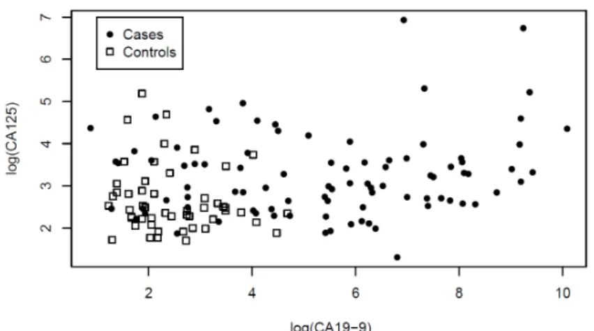
As an example of the application of our method, we use a data set from the literature resulting from a study of 90 pancreatic cancer patients and 51 control patients with pancreatitis [20]. Two serum markers were measured on these patients, the carbohydrate antigen CA19-9 (biomarkerX in our method) and the cancer antigen CA125 (biomarkerY). The marker values were transformed to a natural logarithmic scale and are displayed in Figure1. To make sure that our biomarkers tests results are comparable we used standardized values (i.e. with mean 0 and variance 1) after the natural logarithmic transformation as inputs to our method. Objectives of this example were to see if a weighted average of these two biomarkers could provide a better diagnostic quantity than the individual biomarkers, and to see if the choice of parametric copula in our method would make a substantial difference.
Figure 1. Pancreatic cancer data set
Using the individual biomarkers only, and the empirical ROC method, biomarker CA19-9 leads to empirical AUC equal to 0.8614 and biomarker CA125 to empirical AUC equal to 0.7056. Using Equations (9) and (10), the NPI lower and upper AUC values using only biomarker CA19-9 are 0.8347 and 0.8648, respectively, and when using only biomarker CA125 these values are 0.6883 and 0.7130, respectively. We applied our method with the Clayton, Frank, Gumbel and Normal copulas. The optimal lower and upper AUC values for our method, with corresponding values forα, are shown in Table1.
Copula αˆcL AU Cc αˆcU AU Cc
Normal 0.7160 0.8306 0.7151 0.8896 Frank 0.7077 0.8324 0.7077 0.8920 Clayton 0.7066 0.8364 0.7061 0.8947 Gumbel 0.7215 0.8301 0.7226 0.8880
Table 1. Lower and upper AUC values and corresponding values ofα
These results show that there is very little difference in our method for the four different parametric copulas considered. In terms of the AUC value, the Clayton copula performs best but differences are mainly only in the third decimal. These lower and upper AUC values also all bound the AUC value 0.8614 achieved by using only the best single biomarker CA19-9. For all copulas the performance is, of course, substantially better than for the worst single biomarker CA125, but we aim at using a weighted combination in order to improve on the best individual biomarker. We also applied the empirical method for the linear combination of these two biomarkers, this led to maximum AUC equal to0.8939forαˆ= 0.7188, which is very close to the upper AUC values achieved by our method, with only the Clayton copula providing a slightly better upper AUC value. More important for practical purposes is that the optimal values forαfor all these methods are nearly identical. This example only indicates a hardly noticeable improvement in diagnostic accuracy by combining the two biomarkers over the use of only the single biomarker CA19-9. One possible reason for this is that taking the weighted average is too restrictive if the individual biomarkers for the disease group and for the non-disease group have correlations with different signs, but more importantly our current method with the use of these basic symmetric parametric copulas only considers linear dependence, which is also taken into account in the empirical combination method. The real benefit of our method is likely to show for more complex dependence structures, which will require more flexible copulas to be used, where nonparametric copulas are most likely to be most successful as long as the data sets are suitably large.
5. Concluding remarks
This paper reported on intermediate results from an ongoing study into generalizing the NPI approach to multivariate data, in particular considering the use of such methods for bivariate diagnostic tests. The study has shown that the computational aspects of the method for this application are not a substantial problem, the computation time was mostly determined by the need to find optimal linear combination coefficients, so not for the underlying novel statistical methodology which combines NPI for the marginals with an estimated parametric copula. Simulation studies [16], which we briefly reported, showed a small improvement of our method on the far simpler empirical method in the case of small data sets, but this advantage disappeared for larger data sets. However, thus far only scenarios with linear dependences in the underlying data models have been studied, for which the dependence can be taken into account by the weighted average, also for the empirical method. Real benefit from our novel statistical method is expected when there are more complex dependence structures, but this would require either parametric copulas which reflect the dependence structure, and therefore may require detailed topic knowledge, or the use of flexible nonparametric copulas. We are continuing our research project mainly focussing on the second of these approaches, that is developing predictive inference methods for bivariate data by combining NPI for the marginals with nonparametric copulas, which can also be extended to multivariate data of higher dimension.
In this paper we compared our NPI method with an assumed parametric copula to the basic empirical method described in Section 1. Muhammad [16] also considers a more direct NPI method where, for given value ofα, only the weighted averages of the test results,t1
i and t0j, are used, and NPI is applied per group to provide predictive inference on the weighted average for a future individual from each group. This approach does not attempt to learn dependence between the two diagnostic tests applied to the same person, and it is as simple to apply as the empirical method. Simulation studies [16] showed that the results of that direct NPI method are very close the results of the empirical method, which will also be the case if scenarios with non-linear dependences would be investigated, in which case our new method with the use of a copula is expected to perform substantially better.
In principle our approach can be similarly applied to combination of biomarkers for diagnostic tests if nonparametric copulas are used, so for this specific application a further research topic is in the use of other combination functions of the biomarkers than weighted averages. For practical applications, however, one may wish to stay with functions that lead to a reasonable interpretation of the combination of the biomarkers. It will be interesting to explore combinations of relatively straightforward combination functions with the use of nonparametric copulas in our method and investigate the performance of the resulting methods.
Appendix Proof
The lower probability for the eventTn11+1 > T
0
n0+1, given in Equation (23), is derived as follows
P =P(Tn11+1> T 0 n0+1) = n∑1+1 i=1 n∑1+1 l=1 P(Tn00+1< αX 1 n1+1+ (1−α)Y 1 n1+1, X 1 n1+1∈(x 1 i−1, x 1 i), Y 1 n1+1∈(y 1 l−1, y 1 l)) = n∑1+1 i=1 n∑1+1 l=1 P(Tn00+1< αXn11+1+ (1−α)Yn11+1,(Xn11+1, Yn11+1)∈Bil1) ≥ n∑1+1 i=1 n∑1+1 l=1 h1il( ˆθ1)P(Tn00+1< t 1 i−1,l−1) = n∑1+1 i=1 n∑1+1 l=1 h1il( ˆθ1) n∑0+1 j=1 n∑0+1 k=1 P(αXn00+1+ (1−α)Yn00+1< t1i−1,l−1,(Xn00+1, Yn00+1)∈B0jk) ≥ n∑1+1 i=1 n∑1+1 l=1 h1il( ˆθ1) n∑0+1 j=1 n∑0+1 k=1 1{t0j,k< t1i−1,l−1}h0jk( ˆθ0)
For the lower probability, we want to make the probability for the eventTn11+1> Tn00+1 as small as possible. To this end, the first inequality follows by putting the probability h1il( ˆθ1) corresponding to the block Bil1 to the left-bottom of the block, for all i, l= 1, . . . , n1+ 1. Thus the corresponding combined weighted value is t1
i−1,l−1=αx1i−1+ (1−α)yl1−1. The second inequality follows by putting the probabilityh0jk( ˆθ0)corresponding to the blockB0
jkto the right-top of the block, for allj, k= 1, . . . , n0+ 1, and the corresponding combined weighted value is t0
j,k=αx0j+ (1−α)yk0. Because these configurations of the respective probability masses can actually be achieved, this is the maximum possible lower bound for the probability of interest and hence it is a lower probability.
The upper probability for the eventT1
n1+1> T
0
n0+1, given in Equation (24), is derived as follows
P =P(Tn1 1+1> T 0 n0+1) = n∑1+1 i=1 n∑1+1 l=1 P(Tn0 0+1< αX 1 n1+1+ (1−α)Y 1 n1+1, X 1 n1+1∈(x 1 i−1, x 1 i), Y 1 n1+1∈(y 1 l−1, y 1 l)) = n∑1+1 i=1 n∑1+1 l=1 P(Tn00+1< αXn11+1+ (1−α)Yn11+1,(Xn11+1, Yn11+1)∈Bil1) ≤ n∑1+1 i=1 n∑1+1 l=1 h1il( ˆθ1)P(Tn00+1< t 1 i,l) = n∑1+1 i=1 n∑1+1 l=1 h1il( ˆθ1) n∑0+1 j=1 n∑0+1 k=1 P(αXn00+1+ (1−α)Y 0 n0+1< t 1 i,l,(Xn00+1, Y 0 n0+1)∈B 0 jk ) ≤ n∑1+1 i=1 n∑1+1 l=1 h1il( ˆθ1) n∑0+1 j=1 n∑0+1 k=1 1{t0j−1,k−1< t1i,l}h0jk( ˆθ0)
For the upper probability, we want to make the probability for the event T1
n1+1> T
0
n0+1 as large as possible.
To this end, the first inequality follows by putting the probability h1
the right-top of the block, for all i, l= 1, . . . , n1+ 1. Thus the corresponding combined weighted value is t1i,l=αx1i + (1−α)y1l. The second inequality follows by putting the probability h0jk( ˆθ0) corresponding to the blockBjk0 to the left-bottom of the block, for allj, k= 1, . . . , n0+ 1, and the corresponding combined weighted value ist0j−1,k−1=αxj0−1+ (1−α)yk0−1. This is indeed an upper probability as it is the minimum possible upper bound for the probability of interest.
Acknowledgements
We thank two reviewers for their positive comments about our paper and their useful suggestions for improvement of the presentation.
REFERENCES
1. T. Augustin and F.P.A. Coolen. Nonparametric predictive inference and interval probability. Journal of Statistical Planning and Inference, vol. 124, pp. 251–272, 2004.
2. T. Augustin, F.P.A. Coolen, G. de Cooman and M.C.M. Troffaes (Eds). Introduction to Imprecise Probabilities. Chichester: Wiley, 2014.
3. A. Bansal and M. Sullivan Pepe. When does combining markers improve classification performance and what are implications for practice? Statistics in Medicine, vol. 32, pp. 1877–1892, 2013.
4. F.P.A. Coolen. On nonparametric predictive inference and objective Bayesianism. Journal of Logic, Language and Information, vol. 15, pp. 21–47, 2006.
5. T. Coolen-Maturi. Three-group ROC predictive analysis for ordinal outcomes. Communications in Statistics - Theory and Methods, vol. 46, pp. 9476-9493, 2017.
6. T. Coolen-Maturi, F.P.A. Coolen and N. Muhammad. Predictive inference for bivariate data: combining nonparametric predictive inference for marginals with an estimated copula. Journal of Statistical Theory and Practice, vol. 10, pp. 515–538, 2016.
7. T. Coolen-Maturi, P. Coolen-Schrijner and F.P.A. Coolen. Nonparametric predictive inference for binary diagnostic tests. Journal of Statistical Theory and Practice, vol. 6, pp. 665–680, 2012.
8. T. Coolen-Maturi, P. Coolen-Schrijner and F.P.A. Coolen. Nonparametric predictive inference for diagnostic accuracy. Journal of Statistical Planning and Inference, vol. 142, pp. 1141–1150, 2012.
9. T. Coolen-Maturi, F.F. Elkhafifi and F.P.A. Coolen. Three-group ROC analysis: A nonparametric predictive approach.Computational Statistics & Data Analysis, vol. 78, pp. 69–81, 2014.
10. B. De Finetti. Theory of Probability. London: Wiley, 1974.
11. F.F. Elkhafifi and F.P.A. Coolen. Nonparametric predictive inference for accuracy of ordinal diagnostic tests. Journal of Statistical Theory and Practice, vol. 6, pp. 681–697, 2012.
12. B.M. Hill. Posterior distribution of percentiles: Bayes’ theorem for sampling from a population. Journal of the American Statistical Association, vol. 63, pp. 677–691, 1968.
13. L. Kang, A. Liu and L. Tian. Linear combination methods to improve diagnostic/prognostic accuracy on future observations.
Statistical Methods in Medical Research, vol. 25, pp. 1359–1380, 2016.
14. J.F. Lawless and M. Fredette. Frequentist prediction intervals and predictive distributions. Biometrika, vol. 92, pp. 529–542, 2005. 15. C. Liu, A. Liu and S. Halabi. A min–max combination of biomarkers to improve diagnostic accuracy. Statistics in Medicine, vol. 30,
pp. 2005–2014, 2011.
16. N. Muhammad.Predictive Inference with Copulas for Bivariate Data. PhD thesis, Durham University, UK (available from www.npi-statistics.com), 2016.
17. J.Q. Su and J.S. Liu. Linear combinations of multiple diagnostic markers. Journal of the American Statistical Association, vol. 88, pp. 1350–1355, 1993.
18. M. Sullivan Pepe. The Statistical Evaluation of Medical Tests for Classification and Prediction. Oxford: Oxford University Press, 2003.
19. M. Sullivan Pepe and M.L. Thompson. Combining diagnostic test results to increase accuracy. Biostatistics, vol. 1, pp. 123–140, 2000.
20. S. Wieand, M.H. Gail, B.R. James and K.L. James. A family of nonparametric statistics for comparing diagnostic markers with paired or unpaired data. Biometrika, vol. 76, pp. 585–592, 1989.