Development of Recurrent Neural Networks and Its Applications to Activity Recognition

(1)

Research Online

University of Wollongong Thesis Collection

2017+ University of Wollongong Thesis Collections

2018

Development of Recurrent Neural Networks and Its Applications to Activity

Recognition

Shuai Li

University of Wollongong

Follow this and additional works at: https://ro.uow.edu.au/theses1

University of Wollongong University of Wollongong

Copyright Warning Copyright Warning

You may print or download ONE copy of this document for the purpose of your own research or study. The University does not authorise you to copy, communicate or otherwise make available electronically to any other person any

copyright material contained on this site.

You are reminded of the following: This work is copyright. Apart from any use permitted under the Copyright Act 1968, no part of this work may be reproduced by any process, nor may any other exclusive right be exercised, without the permission of the author. Copyright owners are entitled to take legal action against persons who infringe

their copyright. A reproduction of material that is protected by copyright may be a copyright infringement. A court may impose penalties and award damages in relation to offences and infringements relating to copyright material.

Higher penalties may apply, and higher damages may be awarded, for offences and infringements involving the conversion of material into digital or electronic form.

Unless otherwise indicated, the views expressed in this thesis are those of the author and do not necessarily Unless otherwise indicated, the views expressed in this thesis are those of the author and do not necessarily represent the views of the University of Wollongong.

represent the views of the University of Wollongong.

Recommended Citation Recommended Citation

Li, Shuai, Development of Recurrent Neural Networks and Its Applications to Activity Recognition, Doctor of Philosophy thesis, School of Computing and Information Technology, University of Wollongong, 2018. https://ro.uow.edu.au/theses1/393

Research Online is the open access institutional repository for the University of Wollongong. For further information contact the UOW Library: [email protected]

(2)

Applications to Activity Recognition

Shuai Li

This thesis is presented as part of the requirements for the conferral of the degree:

Doctor of Philosophy

Supervisor: A/PR Wanqing Li Co-supervisor: Prof. Chris Cook

The University of Wollongong

School of Computing and Information Technology

(3)

No part of this work may be reproduced, stored in a retrieval system, transmitted, in any form or by any means, electronic, mechanical, photocopying, recording, or otherwise, without the prior permission of the author or the University of Wollongong.

This research has been conducted with the support of an Australian Government Research Training Program Scholarship.

(4)

I,Shuai Li, declare that this thesis is submitted in partial fulfilment of the requirements for the conferral of the degreeDoctor of Philosophy, from the University of Wollongong, is wholly my own work unless otherwise referenced or acknowledged. This document has not been submitted for qualifications at any other academic institution.

Shuai Li

(5)

Publications

Publications to date resulted from the research presented in this thesis.

• S. Li, D. Florencio, W. Li, Y. Zhao, C. Cook, “A Fusion Framework for Camouflaged Moving Foreground Detection in the Wavelet Domain,” IEEE Transactions on Image Processing, vol. 27, no. 8, pp. 3918–3930, 2018.

• S. Li, W. Li, C. Cook, C. Zhu, Y. Gao, “Independently Recurrent Neural Network (In-dRNN): Building A Longer and Deeper RNN,” IEEE Conference on Computer Vision and Pattern Recognition (CVPR), pp. 5457-5466, Salt Lake City, Utah, Jun. 18-22, 2018.

• S. Li, D. Florencio, Y. Zhao, C. Cook, W. Li, “Foreground Detection in Camouflaged Scenes,”IEEE International Conference on Image Processing (ICIP 2017), Beijing, China, Sep. 17-20, 2017.

• S. Li, C. Li, W. Li, Y. Hou, C. Cook, “Smartphone-sensors based Action Recognition using IndRNN,” The ACM international joint conference on pervasive and ubiquitous computing (Ubicomp 2018), HASCA Workshop, Singapore, Oct. 12, 2018.

• S. Li, W. Li, C. Cook, C. Zhu, Y. Gao, “A Fully Trainable Network with RNN-based Pooling,”Elsevier Neurocomputing,under review.

• S. Li, W. Li, C. Cook, C. Zhu, Y. Gao, “A Deep Attention Model for Action Recognition from Skeleton Data,”IEEE Transactions on Cybernetics,under review.

• S. Li, W. Li, C. Cook, C. Zhu, Y. Gao, “Deep Independently Recurrent Neural Network (IndRNN),”in preparation.

(6)

Abstract

Deep learning, including the Convolutional Neural Network (CNN) and Recurrent Neural Net-work (RNN), has enjoyed great success in the last decade. They have been widely applied in the areas of image and video-related tasks, such as image recognition and action recogni-tion. Despite their great success, there are still some fundamental problems that have not been resolved. This thesis addresses the generic challenges in the CNNs and RNNs as well as chal-lenges specific to their use in human activity recognition. First, an RNN-based pooling function is developed to replace the handcrafted and predefined pooling functions. Together with the other layers of the CNNs, this allows all components of the network to be trained from data. Then an independently recurrent neural network (IndRNN) is proposed to solve the gradient vanishing and exploding problem in the conventional RNNs. Unlike the traditional RNNs, In-dRNN can learn very long-term patterns (over 5000 time steps) and can be stacked to construct very deep networks (over 21 layers). Application of IndRNN to activity recognition is studied where a deep IndRNN based attention model is developed. Finally, applications in complex scenes are explored using camouflaged moving background modelling. Extensive experiments have been conducted to validate the methods proposed in this thesis.

(7)

Chapter 1 Introduction

1.1 Motivation

Deep learning, including convolutional neural networks (CNN) and recurrent neural networks (RNN), has been a great success in the last decade. It has achieved promising performance on many computer vision tasks including image classification, object detection and recognition, and action recognition and prediction. Through the applications of deep learning, CNNs have been shown to be capable of extracting spatial features. By contrast, RNNs have been proven successful in modeling sequential or time-series data such as the temporal patterns in action recognition.

Despite the success of CNNs and RNNs, there are still unresolved issues related to their architectures. For instance, a CNN is generally composed of convolution layers, pooling layers, and fully connected layers. Among them, the convolution layer and the fully connected layer are fully learned while the pooling layer is still handcrafted. Since the power of CNNs comes from their ability to adapt to the data through learning, the natural question to ask is “could pooling be learned from data in a similar way as other components?”. Although some attempts are reported in the literature, the pooling layers are still restricted to a predefined form. Therefore, a pooling function that can be completely learned is highly desirable.

As for RNNs, a long-standing problem is the gradient vanishing and exploding problem re-sulting from the repeated use of the recurrent weight matrix. This makes RNNs very difficult to train and to recognize long-term patterns. Some RNN variants such as long short-term memory

(11)

(LSTM) and gated recurrent unit (GRU) have been developed to address these problems, but the use of specific hyperbolic tangent and the sigmoid activation functions results in gradient decay over layers. Consequently, construction of an efficiently trainable deep RNN is challeng-ing. Moreover, in the current RNN structures, the neurons in each layer are entangled with each other, which makes it very difficult to interpret and understand each neuron’s behaviour.

In addition to the above challenges with respect to the architecture of CNNs and RNNs, there are also challenges at the application to make the results interpretable. For instance, both CNN and RNN have been widely applied to activity recognition, an active field in computer vision intending to understand the human motion from a sequence of images, depth maps and/or skeletons. They are often simply treated as a black box with little being known about why and how it works even though the results are good.

1.2 Contributions

This thesis focuses on improving the CNNs and RNNs by dealing with the above challenges. Specifically, the contributions can be summarized as follows:

• A RNN-based learnable pooling function is proposed. Combined with the other learn-able components, a fully trainlearn-able network (FTN) is developed. Experimental results demonstrate that the proposed RNN based pooling can well approximate the existing pooling functions with just one neuron. Furthermore, experiments have also shown that the proposed FTN can improve the performance over conventional CNNs and achieve state-of-the-art performance in image classification.

• A new type of RNN, referred to as independently recurrent neural network (IndRNN), is proposed, where neurons in one layer are independent of each other and they are con-nected across layers. We have shown that an IndRNN can be easily regulated to prevent the gradient exploding and vanishing problems while allowing the network to learn long-term dependencies. Moreover, an IndRNN can work with non-saturated activation func-tions such as ReLU (rectified linear unit) and be still trained robustly. Multiple IndRNNs

(12)

can be stacked to construct a network that is deeper than the existing RNNs. Experimental results have shown that the proposed IndRNN is able to process very long sequences (over 5000 time steps vs. less than 1000 steps in a conventional RNN), can be used to construct very deep networks (21 layers used in the experiment) and still be trained robustly. Better performances have been achieved on various tasks by using IndRNNs compared with the traditional RNN and LSTM.

• A deep IndRNN based attention model is constructed and applied to skeleton-based ac-tivity recognition. A new triplet loss function is developed to supervise the learning of attention in order to enforce the intra-class attention distance to be smaller than the inter-class attention distance and at the same time to allow multiple attention weight patterns exist for a same class. Significantly better and robust performance is achieved over the traditional RNN models.

• A fusion framework is developed in the wavelet domain to address the camouflaged mov-ing foreground detection problem. Experimental results demonstrate that the proposed method performs significantly better than the existing methods in terms of the camou-flaged foreground detection.

1.3 Thesis Organization

The rest of the thesis is organized as follows.

Chapter 2 provides a literature review of the existing CNN and RNN models. The widely used CNN and RNN architectures are described. The problems in the existing architectures such as the predefined pooling function and the exploding and vanishing gradient are explained in detail.

Chapter 3 presents a RNN-based pooling method and the corresponding fully trainable net-work. Different FTN architectures are explored. Experimental results are presented to demon-strate that the proposed RNN-based pooling can well approximate the existing max and average pooling functions. The effectiveness of the FTN on existing tasks is also demonstrated.

(13)

Chapter 4 presents the independently recurrent neural network (IndRNN). The advantage of IndRNN over traditional RNNs are demonstrated by showing how the existing gradient van-ishing and exploding problem is solved. Different IndRNN network architectures including residual IndRNN are illustrated. Performances on various tasks are presented.

Chapter 5 applies the IndRNN to skeleton based activity recognition and attention based In-dRNN models are explored. The attention behaviour for the skeleton based activity recognition is exploited to construct a new triplet loss function.

Chapter 6 presents a fusion framework to address the camouflaged moving foreground de-tection problem. Foreground and background models are formulated in multiple wavelet bands. The detection results from different bands are fused by considering the properties of different wavelet bands. Experimental results have shown that the proposed method performs signifi-cantly better than the existing methods in terms of the camouflaged foreground detection.

Chapter 7 concludes this thesis with a summary of the main results and suggests future re-search works.

(14)

Chapter 2 Literature Review

This chapter reviews the existing methods in the literature related to the topics in this thesis. CNNs and RNNs are both introduced and their limitations are discussed.

2.1 Convolutional Neural Network (CNN)

Convolutional neural networks (CNNs) are feedforward neural networks. In the following, we first give a brief review on the widely used CNN architectures in the categories of plain CNN and residual CNN, respectively. Then a critical review on pooling, one common component of both architectures, is provided to show the disadvantages of the existing pooling methods.

2.1.1 Plain CNNs

Conventional CNNs are generally constructed based on the basic components of convolutional layer and activation function such as ReLU (recitified linear unit). Every few convolutional layers (3 for example), a pooling layer is inserted to reduce the size of the feature maps, and a few (usually two) fully connected layers are added at the end of the network. Some typical examples are the “LeNet” [1], “AlexNet” [2] and “VGGNet”[3]. Taking the “VGGNet” for example, it is composed of 5 stacks of convolutional layers with a 2×2 pooling layer at the end of each stack, and 2 layers of fully connected layers at the bottom of the network. To accelerate the training of CNNs, batch normalization [4] is usually used.

These network architectures based on the simple components of convolutional layer and

(15)

tivation function are usually referred to as plain CNNs to distinguish them from the residual network. An illustration of a plain CNN is shown at Fig. 2.1 where each convolution layer is composed of a convolution operation, an activation function (ReLU) and batch normalization if needed. There are many more network architectures available in the literature [5]–[7].

It is known that gradient decays over layers and with the current training techniques based on the gradient backpropagation chain rule, such gradient decay behaviour limits the depth of the networks, usually around 20 layers. Fig. 2.2 from [8] shows an example of the performance on CIFAR classification using plain networks with different numbers of layers. It can be seen that with the number of layers increasing from 20 to 50, the performance drops. However, as shown in various reports [9], the deep layers reveal high level information and it is desirable to develop deep networks, which may further improve the performance.

2.1.2 Residual CNNs

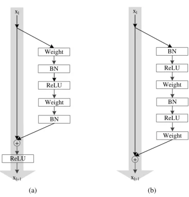
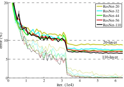
As mentioned above, gradient decays over layers within a plain CNN and thus its depth is con-strained. To overcome this issue, highway networks [10] and residual networks [8] have been developed. In the highway networks, in addition to the connection between two adjacent layers, two nonlinear transforms termed as transform gate and carry gate are introduced. The gates determine how much of the output is produced by transforming the input and carrying it. In the residual networks, the two nonlinear transforms are simplified to a shortcut connection with fixed weights 1 between two layers. A typical component (also known as the residual block) is shown in Fig. 2.3(a). It can be seen that, with the residual connection, the output of deeper layers is the combination of the output of plain CNN block and the output of the earlier layers. Therefore, in the training process, the gradients of a deeper layer can be directly propagated to earlier layers, greatly reducing the gradient vanishing problem across layers. This allows very deep networks (over 100 layers) to be trained. Fig. 2.4 from [8] shows an example of the performance on CIFAR classification task using the residual network with different numbers of layers. It can be seen that the performance increases with increasing number of layers.

(16)

Pooling Layer Convolutional Layer Convolutional Layer Pooling Layer Convolutional Layer Convolutional Layer

Fully Connected Layer

Classification Input (a) Weight BN ReLU (b)

Figure 2.1: Illustration of a plain CNN. (a) Basic architecture, (b) Basic component of a con-volutional layer. 0 1 2 3 4 5 6 0 5 10 20 iter. (1e4) er ro r (% ) plain-20 plain-32 plain-44 plain-56 0 1 2 3 4 5 6 0 5 10 20 iter. (1e4) er ro r (% ) ResNet-20 ResNet-32 ResNet-44 ResNet-56 ResNet-110 56-layer 20-layer 110-layer 20-layer 4 5 6 0 1 5 10 20 iter. (1e4) er ro r (% ) residual-110 residual-1202

Figure 2.2: Demonstration of the performance of plain networks with different number of layers. Courtesy of [8].

(17)

Weight BN Weight BN + xl xl+1 ReLU ReLU (a) BN Weight ReLU BN Weight + xl xl+1 ReLU (b)

Figure 2.3:Basic components of Residual CNN. (a) the conventional type, (b) the preactivation type. Courtesy of [11]

which has a better performance than the simple residual network mentioned above. Several works based on the residual connection have also been proposed in the literature such as the wide ResNets [12] and DenseNet [13], which are not further reviewed here. In addition to the residual networks to increase the depth of the networks, there are also networks with certain structures in each layer such as the “InceptionNet” [14] to increase the width of the network. In the “InceptionNet” [14], in each stack of layers, different convolutional kernels and layer structures are used. Works on combining both the advantage of residual networks and inception structures have also been explored in the literature which show better performance [15].

Despite the great success of residual connections enhanced networks, they still use a hand-crafted pooling component. In the following, the existing pooling techniques are reviewed and its shortcomings are analysed.

(18)

0 1 2 3 4 5 6 0 5 10 20 iter. (1e4) er ro r (% ) plain-20 plain-32 plain-44 plain-56 0 1 2 3 4 5 6 0 5 10 20 iter. (1e4) er ro r (% ) ResNet-20 ResNet-32 ResNet-44 ResNet-56 ResNet-110 56-layer 20-layer 110-layer 20-layer 4 5 6 0 1 5 10 20 iter. (1e4) er ro r (% ) residual-110 residual-1202

Figure 2.4: Demonstration of the performance of the residual network with different number of layers. Courtesy of [8].

2.1.3 Pooling

Motivated from biology [16] where responses of simple cells are fed into a complex cell through some pooling operations, the spatial pooling approach has been found very useful in many computer vision tasks. In CNNs, pooling is an important component for aggregating local features and reducing computational burden. Up to now, the most commonly used pooling methods are still the max pooling and average pooling. The max pooling selects the most salient feature in a pooling region while the average pooling treats the features in a pooling region equally.

However, the features in a local pooling region may be heterogeneous, leading to a loss of information on weak features through max pooling and loss of discriminative information through average pooling [17]. It has been shown that such pooling methods cannot achieve the optimal performance due to this information loss [17]. A theoretical analysis of max pooling and average pooling for classification is provided in [18] based on the i.i.d. Bernoulli distri-bution assumption for binary features and the exponential distridistri-bution for continuous features. It shows that the pooling cardinality and sparsity of the features affect its classification perfor-mance and the perforperfor-mance highly depends on the distribution of the features which is hard to estimate.

(19)

In addition to the max pooling and average pooling, there are some other pooling methods reported in the literature. In [19], a protected pooling method was proposed where a concave function is used to combine the features. The concave function is designed to protect weak codes in order to preserve details. In [20], a stochastic pooling method was proposed where a multino-mial distribution formed from the activation values is used. In this way, the locations with large values are picked as output more frequently than others. Similarly in [21], a rank based pooling was proposed to emphasize information with high rank over others. In [22], spectral pooling was proposed which preforms dimensionality reduction by truncating the representation in the frequency domain. On the other hand, the convolution with sliding strides larger than one pixel [23] can be regarded as an extra convolutional layer with a pooling operation which selects the value of a fixed location. The learning pooling in [24] further simplifies the convolutional operation with an independent linear operation on each channel. These methods are all heavily engineered to certain functions or certain forms which cannot achieve optimal performance on different data, different tasks and different networks.

There are also methods proposed to combine different pooling functions. In [25], a mixed pooling method was proposed where max pooling and average pooling are randomly selected with a stochastic procedure. Similarly, in [26], the max pooling and average pooling are com-bined in a tree structure. In [27] and [28], a geometricl_p-norm pooling was proposed to gen-eralize max pooling and average pooling, which can be represented as(∑N_i₌₁|xIi|

p₎1/p_{. When}

p=1, l_p-norm pooling reduces to average pooling and when p=∞, lp-norm pooling reduces

to max pooling.

Pooling is a process that maps theN×Nto 1 whereN×Nrepresents the size of the local pool-ing region. The existpool-ing poolpool-ing methods certainly lose information in this mapppool-ing process. Compared to the other layers in CNNs such as the convolutional layers and the fully connected layers, the predefined pooling function may not be optimal for a given dataset. Moreover, dif-ferent pooling methods are used in difdif-ferent CNN architectures. Even in one CNN architecture such as the “InceptionNet”[14], different pooling methods are used. While it is difficult to select an appropriate pooling strategy for a better performance, it is also hard to explain how and why

(20)

one pooling strategy works better than others. Therefore, a flexible pooling function that can be learned from data for each pooling layer of a network architecture is highly desirable.

2.2 Recurrent Neural Network (RNN)

Unlike standard feedforward neural networks such as CNNs, recurrent neural networks (RNNs) [29] retain a state that can represent information from the past. Therefore, a RNN is naturally applicable to sequential data and has been widely used in video analysis, speech recognition and neural machine translation. In the following, simple RNN and its variants such as long short-term memory (LSTM) [30] are reviewed.

2.2.1 Simple RNNs

Simple RNNs add a cycle to connect adjacent time steps, termed as recurrent connection. An illustration of a recurrent neuron and its input and output is shown in Fig. 2.5. By unfolding the neuron through the time domain as in Fig. 2.6, a more direct look at the neuron processing inputs of multiple time instances is provided. At time stept, a recurrent neuron receives inputs from the current data pointx(t) and also the previous hidden stateh(t−1). The output of the neuron is calculated based on the hidden stateh(t)at timet. In this way, input from the previous timex(t−1) can influence the current outputy(t) at timet and later by way of the recurrent connections.

It is known that a RNN suffers from the gradient vanishing and exploding problem due to the repeated multiplication of the recurrent weight matrix. This makes it very difficult to train and capture long dependencies. To address this problem, work on initialization and training techniques, such as initializing the recurrent weights to a proper range or regulating the norm of the gradients over time, were proposed in the literature. In [31], an initialization technique was proposed for an RNN with ReLU activation, termed as IRNN, which initializes the recurrent weight matrix to be the identity matrix and bias to be zero. In [32], the recurrent weight matrix was further suggested to be a positive definite matrix with the highest eigenvalue of unity and all the remaining eigenvalues less than 1. In [33], the geometry of RNNs was investigated

(21)

y(t) h(t) x(t) (a) y(t) x(t) h(t-1) h(t) h(t+1) (b)

Figure 2.5:Illustration of a recurrent neuron (a) and its input and output (b).

y(t-2) x(t-2) h(t-3) h(t-2) y(t-1) x(t-1) h(t-1) y(t) x(t) h(t)

(22)

and a path-normalized optimization method for training was proposed for RNNs with ReLU activation. In [34], a penalty term on the squared distance between successive hidden states’ norms was proposed to prevent the exponential growth of IRNN’s activation. Although these methods help ease the gradient exploding, they are not able to completely avoid the problem (the eigenvalues of the recurrent weight matrix may still be larger than 1 in the process of training). Moreover, the training of an RNN with ReLU is very sensitive to the learning rate. When the learning rate is large, the gradient is likely to explode.

There are some RNN variants trying to solve the gradient vanishing and exploding problem by altering the recurrent connections. In [35], a skip RNN was proposed where a binary state update gate is added to control the network to skip the processing of one time step. In this way, less time steps may be processed and the gradient vanishing and exploding problem can be alleviated to some extent. In [36], [37], a unitary evolution RNN was proposed where the recurrent weights are empirically defined in the form of a unitary matrix. In this case, the norm of the backpropagated gradient can be bounded without exploding. In [38], a Fourier Recurrent Unit (FRU) was proposed where the hidden states over time are summarized with Fourier basis functions and the gradients are bounded. However, such methods usually introduce other trans-forms on the recurrent weight which complicates the recurrent units, making it hard to use and interpret.

2.2.2 Long short-term memory (LSTM) and variants

In order to solve the gradient vanishing and exploding problem, long short-term memory (LSTM) [30] is introduced. The key component of LSTM is a constant error carousel (CEC). It is a self-connected linear unit which enforces a constant error flow through time. Multiplicative gates including input gate, output gate and forget gate are introduced, respectively, to protect the memory content stored in CEC, to protect other units from perturbation by current irrelevant memory contents in CEC, and to reset the memory units once the memory is out of date and useless. The gates are controlled by input data, recurrent input and the current cell state (termed as peephole connections).

(23)

A well known LSTM variant is the gated recurrent unit (GRU) [39]. It is composed of a reset gate and an update gate. The update gate selects whether the hidden state is to be updated with a new hidden state, while the reset gate decides whether the previous hidden state is ignored. It has been reported in various papers [40] that GRU achieves similar performance as LSTM and so this not further explained here. There are also some other LSTM variants [40]–[43] reported in the literature. However, these architectures [40]–[43] generally take a similar form as LSTM and show a similar performance as well, and so are not discussed further here.

There is also research on making the LSTM learn longer sequences and construct deeper networks. In [38], auxiliary loss is developed to force LSTM to construct the previous events or predict next events of a sequence, making LSTM process longer sequences. In [44], different deep RNN architectures were investigated including stacking multiple layers to process the hidden states, which results in a deep transition RNN. This is further improved in [45] where a global gating unit is added to allow signals to flow from upper recurrent layers to lower layers. In [46], adaptive computation steps are taken between two time steps, which also forms a deep transition. In [47], a recurrent highway network was proposed where at each time step, multiple layers with highway connections are used to process the input and recurrent input. There is also research on extending LSTM to process multidimensional inputs [48], [49] and bidirectional extension [50].

LSTM and its variants enforce a constant error flow over time steps and use gates on the in-put and the recurrent inin-put to regulate the information flow through the network. However, the use of gates based on the recurrent input prevents parallel computation and thus increases the computational complexity of the whole network. To process the states of the network over time in parallel, the recurrent connections are fixed in [51], [52]. While this strategy greatly simpli-fies the computational complexity, it reduces the capability of their RNNs since the recurrent connections are no longer trainable.

On the other hand, in LSTM and its variants, the hyperbolic tangent and the sigmoid functions are usually used as the activation function resulting in gradient decay over layers. Consequently, construction and training of a deep LSTM based RNN network is practically difficult. By

(24)

contrast, existing CNNs using non-saturated activation function such as ReLU can be stacked into a very deep network (e.g. over 20 layers using the basic convolutional layers and over 100 layers with residual connections [8]) and be still trained efficiently. Although residual connections have been attempted for LSTM models in several works [53], [54], there have been no significant improvement (mostly due to the reason that gradient decays in LSTM with the use of the hyperbolic tangent and the sigmoid functions as mentioned above). Therefore, RNN architectures that can be stacked with multiple layers and efficiently trained are still highly desired.

2.3 Summary

This Chapter first reviews the existing popular deep learning architectures including CNNs and RNNs. Some limitations are discussed and the following issues, in particular, will be addressed in this thesis:

• the handcrafted pooling functions used in the existing CNN architectures, making pooling not adaptive to data.

• the gradient vanishing and exploding problem in the training of RNNs, making RNNs not robust and difficult for processing long sequences.

• the shallow depth of RNN networks because of the gradient decay over layers.

• the difficulty in understanding RNN features due to the entanglement of different neurons.

In addition to the related works described as above, works specifically related to particular topics are further reviewed in each chapter.

(25)

Chapter 3 Fully Trainable Network

3.1 Introduction

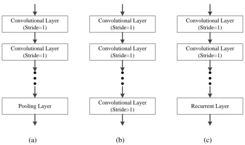
The basic component of a CNN is a stack of convolutional layers (usually more than 2) followed by a pooling layer as shown in Fig. 3.1(a). The convolutional layer can be of many forms such as the traditional convolution structure [3], inception structure [14] and the residual structure [8]. Normalization layers [4] may be used after or before each convolutional layer. The pooling layer is often a max pooling, average pooling or a pooling function as discussed above. Instead of using a pooling layer, a convolutional layer with stride larger than 1 can be used [23] as shown in Fig. 3.1(b) to reduce the dimension of the output features. This chapter proposes a learnable pooling function based on recurrent neural units (RNN). With the capability of a RNN in aggregating features of a sequence, RNNs can effectively aggregate the feature in a local pooling region. Together with the convolutional layers and fully connected layers in CNNs, such a learnable pooling leads to a fully trainable network (FTN).

3.2 The proposed fully trainable network

Unlike the conventional CNNs as shown in Fig. 3.1(a) and Fig. 3.1(b), in the proposed FTN, the basic component is a stack of convolutional layers followed by a RNN layer as shown in Fig. 3.1(c). Specifically, the features in each pooling region are scanned into a sequence as input to the RNN layer. There are many ways to perform the scan. The output of the RNN layer

(26)

Pooling Layer Convolutional Layer (Stride=1) Convolutional Layer (Stride=1) (a) Convolutional Layer (Stride>1) Convolutional Layer (Stride=1) Convolutional Layer (Stride=1) (b) Recurrent Layer Convolutional Layer (Stride=1) Convolutional Layer (Stride=1) (c)

Figure 3.1: Key components in a CNN with (a) a pooling layer, (b) a convolutional layer with stride larger than 1, (c) a recurrent layer.

at the last time stamp is the aggregated feature of the local pooling region, and so is treated as the pooled value. It has been empirically shown that the performance of the FTN is insensitive to the scanning order. Thus simple horizontal scanning is adopted in this chapter. In addition to reducing the dimension of the features, the RNN layer also intends to capture the pattern of the features in a local region. A FTN is constructed by stacking such components.

Notice that in general any type of RNN can be used in the FTN for pooling. This chapter adopts the commonly used LSTM unit. In the following, FTNs are explained in detail with respect to the extension of an LSTM unit for pooling, and the FTN architectures, respectively.

3.2.1 Extension of an LSTM unit for pooling

In the study of CNNs, a general consensus is that for deep networks non-saturated activation functions such as rectified linear units (ReLU) are easier to train than the saturated activation functions such as logistic and hyperbolic tangent functions. In this chapter, it is proposed to extend a conventional LSTM unit with non-saturated activation functions to preform pooling. Such an extension facilitates the training of the LSTM in a consistent way with other layers in a FTN.

(27)

con-stant error flow over time steps. Fig. 3.2 illustrates an LSTM without considering peephole connections. In addition to the CEC, LSTM contains three gates (input gate, forget gate and output gate), and two modulations (input modulation and output modulation). The gates are controlled by the current input and the recurrent input. The activation function for the gates is usually the sigmoid function (σ). The activation functions (ψ) used in input and output mod-ulations are usually the hyperbolic tangent function (tanh). For inputxat each time stept, the LSTM updates its states as follows:

it=σ(Wixt+Riht−1+bi) ft=σ(Wfxt+Rfht−1+bf) ot=σ(Woxt+Roht−1+bo) gt=ψ(Wgxt+Rght−1+bg) ct=itgt+ftct−1 ht=otψ(ct) (3.1) wherext ∈_RM_,_ht−1_∈

RN andM, N represent the dimension of the input feature at time step

t and the number of the neurons in LSTM, respectively. it, ft and ot are the outputs of the input gate, forget gate and output gate, respectively. gt, ct and ht are the output of the input modulation, the cell state and the output of the LSTM, respectively. Wv, Rv and bv are the

weight of the current input, the weight of the recurrent input, and the bias, respectively, for the input gate (v=i), forget gate (v= f), output gate (v=o) and input modulation (v=g). represents the point-wise multiplication.

With the hyperbolic tangent function used as the activation function for input and output modulations, the output of the LSTM is constrained to the range of(−1,1). However, the con-volutional layers and fully connected layers in most CNN architectures employ non-saturated activation functions such as ReLU where their output ranges in[0,+∞). Therefore, the activa-tion funcactiva-tions of the input and output modulaactiva-tions in a LSTM unit are required to be the same

(28)

Input Recurrent + Forget gate Input gate Output gate Input modulation σ σ σ Recurrent Cell

Connection with time-lag

ψ ψ

Output modulation

Figure 3.2:Illustration of a LSTM unit.

as those used in the convolutional layers.

However, change of the activation functions of the input and output modulations in a LSTM unit from a saturated function to a non-saturated function would usually make the training of the LSTM hard to converge according to [31]. In this chapter, one LSTM unit is applied to pool features in a local patch in each channel. Since the processing of all samples in the batch is the same, we take the processing of one data sample as an example to illustrate the LSTM based pooling process. Accordingly, the dimension of input feature from one data sample and the number of neurons are both 1, i.e.,M=1 andN=1. That is, the input, recurrent input, cell state and outputs of all the gates at each time instance and the corresponding weight parameters are all of dimension 1. Let them be noted asxt, ht, it, ft, ot, ct, w_g, r_g, w_v, r_v, b_v, respectively. The following proposition is used as a regulation in the training of LSTM.

Proposition: wg >0 is a necessary condition for a LSTM neuron with ReLU activation

function to converge when processing non-negative input features (xt).

Proof: (Proof by Contradiction) Let the bias of the input modulation be first ignored and considered later, that is,gt=ψ(wgxt+rght−1), where ψ is the ReLU activation function and

xt ≥0. The initial state of the recurrent input (h0) and cell (c0) are both set to be 0 which is used in most networks. Assumew_g≤0. Starting with time instance 1, withx1≥0, the output of the input modulationg1is zero. Since the outputs of all the gates including input gate, output gate and forget gate are non-negative, the output of LSTM (h1) and the cell state (c1) is 0. Hence, the recurrent input and the cell state for the next time instance 2 remains 0. Together

(29)

withx2≥0, the output stays 0. It can be deduced that under such circumstances, the output of LSTM stays 0, which cannot be trained to converge. Therefore, the assumption does not hold and the opposite proposition (w_g>0) is true. On the other hand, bias determines the threshold to activate a neuron. For a LSTM unit, a negative bias for the input modulation deactivates the neuron for small inputs, making the neurons incapable of processing small features. Therefore, the bias for the input modulation is suggested to be constrained to be non-negative as well, in order to preserve the unit’s ability to deal with small inputs.

Experimental results presented in the Section 3.3 of this chapter show that a LSTM unit with ReLU activation function can be trained robustly if this proposition is met.

3.2.2 FTN architectures

The proposed LSTM based pooling can be integrated with convolutional layers in different ways to create different FTN architectures.

• One FTN architecture is that each local pooling region has its own LSTM to be trained and these LSTM units can work as different pooling functions for different regions. In this FTN, pooling is adaptive to local regions.

• The second FTN architecture has one LSTM per layer that is shared by all local regions in the layer. In this case, one pooling operation is performed on all local regions. However, pooling at different layers can be different depending on the training. For instance, the LSTM in one layer may act like a max pooling and the LSTM in another layer may act like an average pooling or a different function that the LSTM would best approximate for the training data.

• The third FTN architecture is one LSTM unit shared by all pooling layers. This is equiv-alent to the conventional CNN where either max or average pooling is adopted.

Obviously, the first architecture is the most powerful one as it is adaptive to each region. How-ever, it also has the maximum number of parameters to be trained for the pooling, and the

(30)

network may become overfitting if it is not well regularized. With the large number of pa-rameters, the memory needed to train the network is also large and the training takes longer time. Thus in the experiments, the second and third architectures are evaluated and compared to illustrate the benefits of the proposed LSTM based pooling over the traditional pooling.

3.3 Experimental Results

Experiments were first conducted to validate that one LSTM unit can well approximate the max and average pooling functions, thus showing the proposed LSTM based pooling is appropriate to be used as pooling in the network. Next, experiments were devised to illustrate that an adaptive pooling such as the proposed LSTM based pooling can outperform the predefined max or average pooling and analysis on the learned pooling function is provided. Finally, the performance of FTN is verified on conventional classification tasks by comparing with existing state-of-the-art methods.

3.3.1 LSTM for average and max pooling

The average pooling is a simple linear function which can be easily approximated by LSTM. However, the max pooling function is a highly non-linear function. In the following, an experi-ment was devised to show that one LSTM unit is able to approximate the max pooling function to a high degree of accuracy.

Simulation setup: ReLU was assumed as the activation function for the convolutional layers that a LSTM unit would work with. Experiments for other non-saturated activation functions can be conducted in a similar way. For ReLU (max(0,x)), the range of the output in theory is [0,+∞). In experiments of image classification, it is observed that the outputs generally fall in the range[0,300]. Therefore, random numbers in this range were generated as the input to simulate the output of a convolutional layer. Since the pooling sizes used most in CNN are 2×2, 3×3 and 4×4, three sets of experiments were conducted with lengths of the input being 4, 9 and 16, respectively. One LSTM unit with the modified activation function (ReLU here) was used. The algorithms are implemented using Theano [55] and Lasagne [56], and run on

(31)

Table 3.1:MAE(10−5) of one LSTM unit with the modified activation function to approximate a max pooling function.

T1 T2 T3

Pool size 2×2 8.97 8.91 9.19 Pool size 3×3 4.42 4.39 4.40 Pool size 4×4 5.41 5.28 5.32

GPU (Titan XP).

Training: The LSTM was trained by minimizing the mean absolute error (MAE) between the output and the max value of the input to approximate the max pooling using mini-batch gradient descent with Nesterov momentum [57] and the batch size was set to 128. The initial learning rate was set to 0.1 and the momentum was set to 0.9. Regularizations such as weight decay and dropout were not used since infinite training examples can be generated. 104batches were considered as an epoch and one epoch was used for validation. The learning rate was decreased by a factor of 10 when the validation accuracy stopped improving. The input weight and bias of the input modulation in the LSTM unit was initialized and regulated as described in subsection 3.2.1.

Testing: The batch size used for testing is the same as that for training. One epoch (104 batches) of data was generated for testing. The performance of the trained network is evaluated on three sets of input data: T1: random numbers in the range [0,300]; T2: 50% of random numbers in the range [0,300] and the other 50% being 0; T3: 20% of random numbers in the range [0,300] and the other 80% being 0. The tests were designed to simulate the cases of general patches, relatively sparse patches and highly sparse patches considering that the responses of the convolutional neurons can be sparse. The performance for different pooling sizes are tabulated in Table 3.1.

From Table 3.1, it can be seen that one LSTM unit is able to well approximate the max pooling function as the errors are all smaller than 10−4 (which is negligible compared to the data range of[0,300]). It can be also seen that the performance is insensitive to the pooling sizes. The experiment on using the trained model for data of a bigger range is also conducted

(32)

Table 3.2: MAE(10−3) of one LSTM unit trained with data range[0,300]to approximate a max pooling function on data range[0,3000].

T1 T2 T3

Pool size 2×2 0.994 0.993 0.994 Pool size 3×3 2.03 2.03 2.03 Pool size 4×4 9.10 9.10 9.10

to demonstrate that the learned pooling function can well process the data that is larger than the trained data range or at least in a relatively larger range. Experiments were conducted assuming the range of the test data is [0, 3000] while the LSTM was trained on data within [0, 300]. The results in terms of MAE are shown in the Table 3.2. It can be seen that although the MAE is larger than that for data in the range [0, 300], it is still relatively small (all smaller than 0.01) considering the large input range (3000). This demonstrates that the learned pooling function can deal with the data larger than the trained data. To further demonstrate that our RNN-based pooling can approximate max pooling well, the pre-trained RNN-based pooling is used for classification on ImageNET as shown in the following.

pre-trained LSTM-based pooling for ImageNET Classification

Limited by our computing resources, we are not able to train a large network on ImageNET. We only show the result of replacing the pooling function in the existing pre-trained network with our proposed RNN based pooling function (pre-trained as in Subsection 3.3.1) in Table 3.3. It can be seen that the network combined with our proposed pooling function almost achieves the same performance as the original network (within marginal error), which validates that our proposed pooling function can well approximate the max pooling function. For VGG19 network, the network with the proposed RNN based pooling surprisingly achieves slightly better performance than the original network in terms of the top5 error rate. Since the network is not trained after replacing the pooling, we conjecture that the slight increase may be due to the small discriminability introduced by the proposed RNN based pooling. It can be seen that the slight error in the max pooling approximation task does not affect the performance of the whole

(33)

Table 3.3: Results on ImageNET in terms of validation error rate (%) using the pre-trained network with max pooling and the pre-trained LSTM based pooling (proposed), respectively.

Top-1 Top-5

Max pooling Proposed (No training) Max pooling Proposed (No training)

VGG16 26.12 26.11 8.22 8.21

VGG19 26.03 26.03 8.13 8.12

Table 3.4: Classification result comparison on CIFAR-10 in terms of test error rate (%) using different sizes of networks.

Network Max pooling Average pooling Proposed pooling (shared) Proposed pooling

Conv 8 57.44 56.18 50.96 50.52

Conv 16 32.75 32.86 28.58 25.72

Conv 32 18.77 20.82 16.11 15.48

Conv 64 13.27 14.75 12.04 11.83

network. Considering that RNNs are universal approximators and can be further trained with data and task, it is reasonable to assume that the proposed FTN with the RNN based pooling can outperform the traditional CNNs with max pooling. Note that this experiment is only used to demonstrate that a learned max pooling function works very well by just replacing the pooling function in the existing models without further training. In the following, the performance of FTN over CNNs will be illustrated and the learned pooling functions will be investigated.

3.3.2 Analysis of the LSTM based pooling

Performance on different sizes of networks

To illustrate the effectiveness of the proposed LSTM based pooling, experiments were con-ducted on the popular CIFAR-10 dataset. The dataset was preprocessed in the same way as in [58]. That is, the dataset is preprocessed with global contrast normalization and ZCA whitening, and the images were padded with four zero pixels at borders. While training, 32×32 random crops with random horizontal flipping were used as input.

A CNN, composing of two stacks of 3×3 convolutional layers (2 layers in each stack) with a pooling layer at the end of each stack, 2 fully connected layers, and an additional fully

(34)

con-nected layer of 10 units together with a softmax output layer for classification was used. The same number of units, denoted by N, were used in the convolutional layers and the 2 fully connected layers. The corresponding network is denoted as Conv N. To better demonstrate the effectiveness of the LSTM based pooling, a large local pooling region, namely 4×4 and 8×8 for the first and second pooling layers, respectively, were used. After the pooling layers, the size of the input to the fully connected layers is 1×1, thus the fully connected layers work in the same way as convolutional layers. A leaky ReLU unit with leakiness of 0.3 was used as the activation function for both convolutional layers and fully connected layers, which has been re-ported [59] to achieve a good performance on classification. Batch normalization [4] was used for convolutional layers and dropout (drooping rate 50%) was applied after each fully connected layer. Total norm constraint on the gradients as in [60] was used to stabilize the training. The initial learning rate was set to 0.01 and decreased by a factor of 10 after 50k and 40k iterations, respectively, and the training ended at the 122K-th iteration. SGD with Nesterov momentum [57] of 0.9 was used for training, and the batch size was 100.

The results are shown in Table 3.4. The column of “proposed pooling” and “proposed pool-ing (shared)” represent the second and third architectures described in subsection 3.2.2, respec-tively. That is to say, for “proposed pooling (shared)”, both pooling layers share one LSTM unit while for “proposed pooling”, each pooling layer has one LSTM unit. From the table, three observations can be made:

• The networks with the proposed LSTM pooling always improve the accuracy (lower the error rate) compared with the corresponding CNNs coupled with the traditional max pool-ing or average poolpool-ing function.

• When the network is very small such as Conv 8, the performance improvement due to the LSTM based pooling is significant, up to 7 percentage points. As the network size increases, the improvement decreases. It is conjectured that although a fixed pooling function may not optimally aggregate the local features, extra convolution kernels may compensate this to some extent. Thus with the increase of the convolution units, the gain

(35)

(a) (b)

(c) (d)

Figure 3.3: Illustration of the location selection in the max pooling over different sizes of the networks.

of using a better pooling function over traditional pooling method drops. However, given the data and task, if the network is too large, it may become overfitting. Therefore, a better pooling function to aggregate the features while reducing the requirement of neurons is highly desired.

• The performance of the second architecture of FTN is better than the third, i.e., different LSTM units for different pooling layers improves the performance of FTN. This indicates that the optimal pooling functions for different pooling layers are likely to be different.

(36)

(a)

(b)

Figure 3.4: Outputs of the learned pooling function from networks of different sizes in com-parison with the max pooling and average pooling. (a) Learned function of the first pooling layer, (b) learned function of the second pooling layer.

(37)

Analysis of the learned pooling function

As shown in Table 3.4 and described above, the performance gap between the proposed pooling and the existing pooling methods becomes smaller with the increase of the number of convo-lution kernels, especially for the max pooling. Since pooling is aN×N to 1 mapping process, information of certain locations in the pooling region may be lost in the existing pooling pro-cess, leading to a degraded performance of the network. In the following, we first show that networks are trained to preserve information of different locations in a pooling region.

For a CNN, max pooling is used independently for each channel. And for each channel, it selects the value of one location (which is the location with the maximal value) as the output and the information at that location is implicitly carried forward in this channel. That is to say, for the pooling process over multiple channels, information from a number of locations may be selected and preserved by one or more channels. Fig. 3.3 shows the histogram of the number of locations that have been selected by at least one channel. The output of max pooling for 5000 randomly selected local patches in the dataset are used for different networks. The pooling size is 4∗4 in all networks, leading to a local region of 16 locations. For the Conv 8 network, the number of neurons is 8, and thus at most 8 locations can be selected by the max pooling (when locations selected by different channels are all different). Fig. 3.3(a) shows that generally more than 4 locations have been selected in one or more channels, and for some pooling regions, all 8 locations are selected. For the Conv 16 network shown in 3.3(b), generally more than 6 locations have been selected. For the Conv 64 network shown in 3.3(b), in over 50% pooling regions, all 16 locations have been selected. It is reasonable to assume that when the number of the neurons is large enough, information from all locations may be implicitly carried forward after the pooling operation. It indicates that networks (convolution kernels) are trained to sample information from all locations. Consequently, with the increase of the number of neurons, the effect of a good pooling operation may be reduced since information from more locations could be sampled through different channels. However, in this case, noise may also be kept by different channels and when the number of neurons is very large, the network becomes overfitting and degrades the performance. On the other hand, since LSTM

(38)

can aggregate information of a sequence, it can adaptively sample more information from all the pooling locations rather than just the existing pooling functions. Therefore, the performance of the proposed FTN is significantly better than the traditional CNN when the number of neurons used is small. Moreover, compared to CNN, FTN can lower the requirement of the number of neurons for a better performance in order to avoid overfitting.

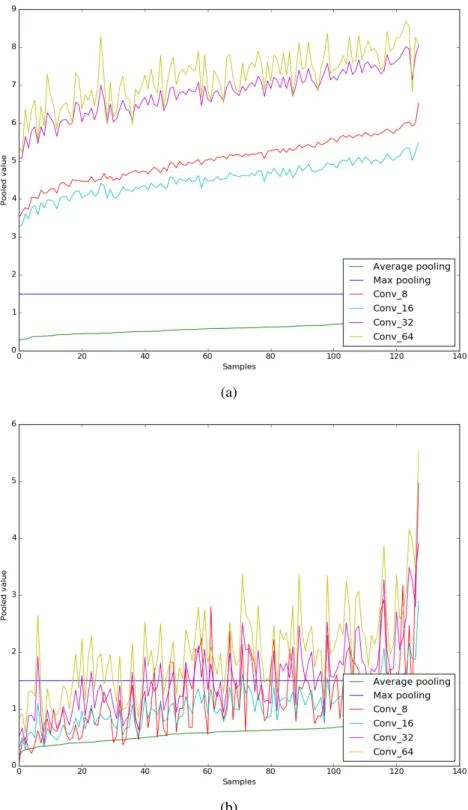
To illustrate the learned LSTM based pooling functions for different pooling layers in the network of different sizes, the output of the pooling function in comparison with the max pool-ing and average poolpool-ing is shown in Fig. 3.4. For better illustration, random values with a fixed maximum value (1.5) are used as input and the output is rearranged according to the magnitude of the average pooling result. Fig. 3.4(a) shows the output of the learned pooling function from the first pooling layer. “Conv N” represents the outputs obtained from the different pool-ing functions learned from their correspondpool-ing “Conv N” networks, respectively. Note that the mean value of each pooling result can be compensated by the bias of the neurons in the fol-lowing layer, thus the variation of each pooling result is more meaningful. It can be seen that the learned pooling functions of the first pooling layer work similarly as the average pooling. Especially for the small networks such as “Conv 8” and “Conv 16”, the output highly correlates with the output of average pooling and the variation is relatively small. This indicates that aver-age pooling may perform better than max pooling for the first pooling layer of small networks, which agrees with our results shown in Table 3.4.

For the learned pooling function of the second pooling layer as shown in Fig. 3.4(b), it can be seen that the variation is very large, i.e., highly sensitive to the different patterns of the inputs. First, compared with the input to the first pooling layer, each input to the second pooling layer corresponds to a larger region of the original image and thus more useful information for the task. Second, it is known that outputs of the higher layers in the network capture high level information, and information at different locations may produce different contexts for the final classification task. For example, the same input with different orders may produce different results. Thus it is very important for the pooling layer to aggregate information while capturing useful patterns. This can be done using our proposed pooling but not possible for the traditional

(39)

Table 3.5:Complexity comparison between CNN and the proposed FTN in terms of time (sec per batch). Train with cudnn Train without cudnn Test with cudnn Test without cudnn CNN 0.013 0.021 0.0027 0.0037 FTN 0.033 0.035 0.0068 0.0076

max pooling and average pooling, leading to the performance improvement shown in Table 3.4. By comparing the learned pooling functions of two layers, it can be seen that the optimal pooling functions for different pooling layers are quite different. In the traditional CNNs, max pooling and average pooling are often selected empirically. In the “InceptionNet” [14], both max pooling and averaging pooling are adopted at different layers also empirically. In such a case, the whole network is unlikely to achieve the best performance. On the other hand, our proposed LSTM based pooling is able to be adaptive for each layer to the training data and thus achieve a better performance, as shown in Table 3.4 by comparing the performance the “Proposed pooling (shared)” and “Proposed pooling”.

Complexity

As mentioned in Subsection 3.2, the proposed LSTM based pooling first transforms theN×N

local region to a sequential input of lengthN×N. Then it processes this sequential input. For example, for the general 2×2 pooling, LSTM needs to process inputs of 4 time steps. It is known that the update of LSTM at each time step in Eq. (3.1) can be regarded as convolution with multiple channels. So the complexity of the proposed pooling is similar to performing 4 convolutional layers. To evaluate its complexity, a similar network as the Conv 64 network (except that the pooling size is set to be 2×2) was used. Batch size was set to be 1 to purely monitor the computation without considering memory issues. The program was implemented based on Theano [61] and Lasagne, and runs on a TITAN X GPU. The time used in the training and testing process is shown in Table 3.5. Since convolution is heavily optimized in cudnn (the deep neural network library developed in NVIDA CUDA), we show both results obtained with

(40)

cudnn and without cudnn. It can be seen that the complexity of training the above FTN network is about two-three times that for training CNN. This is consistent with our above analysis that the complexity of the proposed LSTM based pooling is similar to performing 4 convolutional layers. Since pooling is only applied a few times depending on the size of the input (around 5 times for input of size 256), the complexity of training FTN is bounded. Compared to the current networks over 100 layers, the increase in training time is acceptable considering the benefit of having a learnable pooling function to improve the performance. Moreover, compared to the image modelling methods that use RNN to process the whole image in a sequential manner, the time increase due to the proposed pooling is relatively very small. It is worth noting that since the proposed pooling is learned from data for a network, it can be used as a tool to develop new pooling functions for different applications.

3.3.3 Classification performance on PASCAL VOC 2012

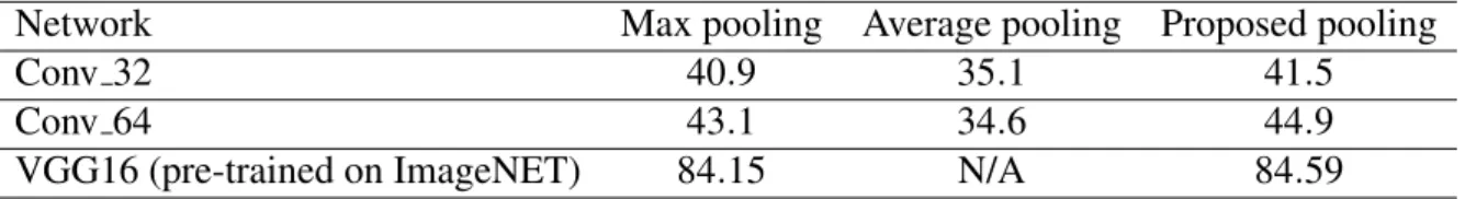
This subsection reports the results on PASCAL Visual Object Classes Challenge (VOC) 2012 dataset [62]. VOC contains 22531 images in 20 classes for training (5717) and validation (5823), and testing (10991). For this dataset, since there may be multiple labels for each image, instead of using softmax as in Subsection 3.3.2, sigmoid is used at the end of the network to indicate whether each class presents in an image. To demonstrate the performance of our RNN-based pooling over the existing pooling methods, networks similar to those in Subsection 3.3.2 are chosen where two stacks of convolutional layers are used and the number of parameters used for the convolutional layers is the same, referred to as Conv N. Two pooling layers are used with pooling size 4×4 and 8×8, respectively, and two fully connected layers are used at the end with 256 neurons. The dataset is preprocessed into size 134×134 and random crops of size 128×128 are used as input. Considering the size of the dataset, batch size is set to 16. Other settings are the same as in Subsection 3.3.2, where SGD with Nesterov momentum [57] of 0.9 was used and the initial learning rate was set to 0.01. Average pooling, max pooling and the proposed RNN-based pooling are evaluated for all networks. Moreover, the VGG16 model [3] pre-trained on ImageNET is also fine-tuned on this dataset with the original max pooling

(41)

Table 3.6:Classification result comparison on PASCAL VOC 2012 in terms of mAP (%) using different networks.

Network Max pooling Average pooling Proposed pooling

Conv 32 40.9 35.1 41.5

Conv 64 43.1 34.6 44.9

VGG16 (pre-trained on ImageNET) 84.15 N/A 84.59

and the pre-trained LSTM-based pooling (replacing the max pooling), respectively. For the fine-tuning process, the last layer of 1000 neurons with softmax function in the VGG16 model is replaced by 20 neurons with sigmoid function for the classification. The dataset is prepro-cessed into size 256×256 and random crops of size 224×224 as in [3] are used as input. Initial learning rate of 0.01 is used first to train the last layer with other layers fixed and then dropped by a factor of 10 to train all the layers.

The performance is shown at Table 3.6 in terms of mean Average Precision (mAP) [62]. For the fine-tuning process, the result on the test set (evaluated by the PASCAL VOC server) is presented while for the others, the result on the validation set is presented for simplicity. From Table 3.6, it can be seen that the proposed RNN-based pooling consistently improves the performance over max pooling and average pooling. Mover, even for the fine-tuning process where the parameters are first learned based on max pooling, the proposed RNN-based pooling still improves the performance of the overall model by fine-tuning on the dataset (relatively small compared with ImageNET).

3.3.4 Classification performance on CIFAR-10 and CIFAR-100

In this Subsection, the widely used CIFAR-10 and CIFAR-100 datasets were used to evalu-ate the performance of the proposed FTN (the second architecture). A similar network as the VGG16 architecture [3] was used for classification due to its popularity. Fig. 3.5 shows the detailed architecture. It is composed of 5 stacks of convolutional layers with a 2×2 pooling layer at the end of each stack, and 2 layers of fully connected layers in the end. Since the spatial size of the input to the fully connected layers is 1∗1, the fully connected layers works in the

(42)

32*32*64 16*16*128

8*8*256 4*4*512

2*2*512 1*1*512

Convolutional layer Pooling layer

Figure 3.5: Illustration of the network architecture used for classification on CIFAR-10 and CIFAR-100.

Table 3.7:Comparison of the proposed FTN and CNNs on CIFAR-10 and CIFAR-100 in terms of test error rate (%).

Network CIFAR-10 CIFAR-100

DSN[63] 7.97 34.57 NIN[64] 8.81 35.68 Maxout[65] 9.38 38.57 All-CNN[23] 7.25 33.71 Highway Network[66] 7.60 32.24 ELU[58] 6.55 24.28 LSUV[59] 6.06 29.96 LSUV*[59] 5.84 N/A LEAP[24] 7.17 29.80 Stochastic Pooling[20] 15.13 42.51

Rank based Pooling[21] 13.84 43.91

Mixed Pooling[25] 10.80 38.07

Tree Pooling[26] 6.67 33.13

Tree+Max-Avg Pooling[26] 6.05 32.37

Baseline 6.29 27.09

Proposed FTN 5.79 26.89

With extreme data augmentation[67]

Fract. Max-pooling [67] 4.50 26.39

All-CNN[23] 4.41 N/A

LSUV*is obtained with deep residual network using maxout as activation function. N/A represents the result is not provided in the corresponding paper.

(43)

(a)

(b)

Figure 3.6: Test error comparison between the proposed FTN and the traditional CNN, (a) over the entire training process, (b) over the first 20 epochs.

(44)

same way as convolutional layers. In the figure, the convolutional layer includes the convo-lution operation, batch normalization and activation function, and the size of the input to the convolutional layer and the number of neurons are also shown in the figure. A fixed 10/100 units fully connected layer together with a softmax output layer are added in the end for clas-sification of CIFAR-10 and CIFAR-100, respectively. The leaky ReLU unit with leakiness of 0.1 was used as activation functions for both the convolutional layers and fully connected lay-ers. Dropout was used after the pooling layers (dropping rate 30%) and fully connected layers (dropping rate 50%) to regularize the training. The preprocessing of the dataset and the training procedure are the same as in Subsection 3.3.2. For the proposed FTN, the pooling layers were replaced with LSTM units, one for each pooling layer. It is worth noting that one LSTM unit only introduces 12 parameters. On the contrary, one convolutional unit generally introduces

N×N×C_l₋₁+1 units whereNis the filter size,C_l₋₁is the number of channels of the input to the current unit, and+1 indicates the bias. Compared to the large amount of parameters used in CNN, the increased number of parameters due to a LSTM unit is negligible.

The results of the FTN and the comparison to the existing methods using the similar plain CNN architectures are shown in Table 3.7. It can be seen that under similar training conditions (without the extreme data augmentation [67]), the proposed FTN outperforms the baseline net-work with max pooling and achieves better performance than other pooling methods using the similar network architecture. Although LSTM has been reported to be difficult to train in the literature, it is found that the proposed FTN converges very fast in the experiments, even faster than a CNN with traditional max pooling. The test errors of the proposed FTN and CNN versus the training epochs are shown in Fig. 3.6(a). Fig. 3.6(b) shows the zoomed-in curve of the testing errors of the first 20 epochs. It can be clearly seen that the proposed FTN achieved a relatively higher performance in less iterations than the CNN.

(45)

3.4 Summary

In this Chapter, a fully trainable network (FTN) is proposed, where the handcrafted pooling layer in the traditional CNNs is replaced with RNN in the proposed FTN. Due to the capability of a LSTM or RNN in general in modelling sequential data, the proposed learnable pooling can be trained to capture patterns of the data in the pooling regions. Experimental results have verified the efficacy of the proposed RNN based pooling and FTN. Specifically, we have shown that only one LSTM unit based pooling can approximate the existing pooling functions with a very high accuracy. Moreover, the performance on image classification tasks including the CIFAR-10, CIFAR-100 and PASCAL VOC demonstrates that the proposed FTN with the LSTM based pooling achieves better performance than the existing pooling methods.

(46)

Chapter 4 Independently Recurrent Neural Network

(IndRNN)

4.1 Introduction

Recurrent neural networks (RNNs) [29] have been widely used to solve problems of sequential data such as action recognition [68] and language processing [39], and have achieved impressive results. Compared with the feed-forward networks such as the convolutional neural networks (CNNs), a RNN has a recurrent connection where the last hidden state is an input to the next state. The update of states can be described as follows:

ht=σ(Wxt+Uht−1+b) (4.1)

wherex_t ∈_RM _and _h

t ∈RN are the input and hidden state at time step t, respectively. W∈

RN×M,U∈RN×N andb∈RN are the weights for the current input and the recurrent input, and the bias of the neurons. σ is an element-wise activation function of the neurons, andN is the number of neurons in this RNN layer. By unfolding RNN in time, this can be illustrated as in Fig. 4.1(a).

Training of the RNNs suffers from the gradient vanishing and exploding problem due to the repeated multiplication of the recurrent weight matrix. Several RNN variants such as the long short-term memory (LSTM) [40], [43] and the gated recurrent unit (GRU) [39] have been pro-posed to address the gradient problems. However, the use of the hyperbolic tangent and the

Development of Recurrent Neural Networks and Its Applications to Activity Recognition

Research Online

Research Online

Development of Recurrent Neural Networks and Its Applications to Activity

Development of Recurrent Neural Networks and Its Applications to Activity

Recognition

Recognition

Applications to Activity Recognition

Publications

Abstract

Contents

Chapter 1

Introduction

1.1

Motivation

1.2

Contributions

1.3

Thesis Organization

Chapter 2

Literature Review

2.1

Convolutional Neural Network (CNN)

2.1.1

Plain CNNs

2.1.2

Residual CNNs

2.1.3

Pooling

2.2

Recurrent Neural Network (RNN)

2.2.1

Simple RNNs

2.2.2

Long short-term memory (LSTM) and variants

2.3

Summary

Chapter 3

Fully Trainable Network

3.1

Introduction

3.2

The proposed fully trainable network

3.2.1

Extension of an LSTM unit for pooling

3.2.2

FTN architectures

3.3

Experimental Results

3.3.1

LSTM for average and max pooling

3.3.2

Analysis of the LSTM based pooling

3.3.3

Classification performance on PASCAL VOC 2012

3.3.4

Classification performance on CIFAR-10 and CIFAR-100

3.4

Summary

Chapter 4

Independently Recurrent Neural Network

(IndRNN)

4.1

Introduction