All-Pairs Shortest Path Algorithms Using CUDA

(1)

Durham E-Theses

All-Pairs Shortest Path Algorithms Using CUDA

KEMP, JEREMY,MARK

How to cite:

KEMP, JEREMY,MARK (2012) All-Pairs Shortest Path Algorithms Using CUDA, Durham theses, Durham University. Available at Durham E-Theses Online: http://etheses.dur.ac.uk/5564/

Use policy

The full-text may be used and/or reproduced, and given to third parties in any format or medium, without prior permission or charge, for personal research or study, educational, or not-for-prot purposes provided that:

• a full bibliographic reference is made to the original source • alinkis made to the metadata record in Durham E-Theses

• the full-text is not changed in any way

The full-text must not be sold in any format or medium without the formal permission of the copyright holders. Please consult thefull Durham E-Theses policyfor further details.

Academic Support Oce, Durham University, University Oce, Old Elvet, Durham DH1 3HP e-mail: [email protected] Tel: +44 0191 334 6107

(2)

All-Pairs Shortest Path Algorithms Using

CUDA

Jeremy M. Kemp

Utilising graph theory is a common activity in computer science. Algorithms that perform computations on large graphs are not always cost effective, requir-ing supercomputers to achieve results in a practical amount of time. Graphics Processing Units provide a cost effective alternative to supercomputers, allow-ing parallel algorithms to be executed directly on the Graphics Processallow-ing Unit. Several algorithms exist to solve the All-Pairs Shortest Path problem on the Graphics Processing Unit, but it can be difficult to determine whether the claims made are true and verify the results listed. This research asks “Which All-Pairs Shortest Path algorithms solve the All-Pairs Shortest Path problem the fastest, and can the authors’ claims be verified?” The results we obtain when answering this question show why it is important to be able to collate existing work, and analyse them on a common platform to observe fair results retrieved from a single system. In this way, the research shows us how effective each algorithm is at performing its task, and suggest when a certain algorithm might be used over another.

(3)

All-Pairs Shortest Path Algorithms Using

CUDA

Jeremy M. Kemp

Submitted for the degree of MScR Computer Science to the School of Engineering and Computing Sciences, Durham University, 2012

(4)

List of Figures

2.1 A representation of a sequential algorithm on the CPU (Barney, 2010) . . . 11 2.2 A representation of a parallel algorithm on multiple CPU

(Bar-ney, 2010) . . . 12 2.3 A Diagram Showing Two Threads in Circular Deadlock . . . 14 2.4 CUDA Hardware Model, Demonstrating Memory Hierarchy and

Overall Hardware Architecture of CUDA GPUs (NVIDIA, 2009) 21 4.1 Graph Representation as a Compacted Adjacency List (Harish

et al., 2009) . . . 39 4.2 Equation to Skip OverxThread Blocks . . . 48 4.3 Equation to Skip Overy Thread Blocks . . . 48 4.4 Overview of Katz’s Data Access During Phase 3 (Katz and Kider,

2008) . . . 49 4.5 Overview of Katz’s Algorithm Executing where 0,0 is the Primary

Block (Katz and Kider, 2008) . . . 49 5.1 Experimental PC Specifications . . . 54 5.2 Quoc-Nam Tran CUDA Floyd-Warshall and CPU Floyd-Warshall 56 5.3 Quoc-Nam Tran CUDA APSP and CPU Floyd-Warshall . . . 58 5.4 Katz and Kider’s Algorithm, CPU Floyd-Warshall and CPU Blocked

Floyd-Warshall . . . 59 5.5 Katz and Kider’s Algorithm, Modified Algorithm, CPU

Floyd-Warshall and CPU Blocked Floyd-Floyd-Warshall . . . 61 5.6 Katz and Kider’s Shared Algorithm and Modified Algorithm . . 62 5.7 Katz and Kider’s Shared and Modified Algorithms with

Floyd-Warshall and Blocked Floyd-Floyd-Warshall . . . 63 5.8 Harish and Narayanan’s Algorithm with CPU Floyd-Warshall . . 65 5.9 All CUDA Algorithms . . . 66

(7)

List of Tables

2.1 Flynn’s Taxonomy . . . 15

2.2 Single Instruction, Single Data . . . 15

2.3 Single Instruction, Multiple Data . . . 16

2.4 Multiple Instruction, Single Data . . . 16

2.5 Multiple Instruction, Multiple Data . . . 17

2.6 Device Memory Features (NVIDIA, 2012) . . . 20

(8)

Glossary

API Application Programming Interface.

APSP All-Pairs Shortest Path.

CPU Central Processing Unit.

CUDA Compute Unified Device Architecture.

device memory is the largest storage available on the GPU, similar to RAM on a PC.

DRAM Dynamic Random Access Memory.

GB Gigabyte (109 _bytes).

GPGPU General-Purpose Computing on Graphics Processing Units.

GPU Graphics Processing Unit.

KB Kilobyte (103_bytes).

kernel is a CUDA function that allows code to be executed in parallel on the GPU.

MB Megabyte (106 _bytes).

MIMD Multiple Instruction, Multiple Data.

MISD Multiple Instruction, Single Data.

RAM Random Access Memory.

SIMD Single Instruction, Multiple Data.

SISD Single Instruction, Single Data.

SSSP Single-Source Shortest Path.

thread block is a collection of CUDA threads that all execute on a single CUDA core.

warp is a group of CUDA threads that reside in a thread block, and that all execute the same instructions at the same time. Usually, in groups of 32.

(9)

Copyright

The copyright of this thesis rests with the author. No quotation from it should be published without the author’s prior written consent and information derived from it should be acknowledged.

Acknowledgements

I would like to thank my supervisor, Professor Iain Stewart, for his many useful and insightful suggestions in regards to this work and the advice given during our many meetings! I would also like to thank my family for their continued support during my time at Durham, as well as Charlotte Hawkins for checking my work many times over!

(10)

Chapter 1

Introduction

1.1 Research Overview

Parallel computing on the Graphics Processing Unit (GPU) has been selected for use in an increasing number of systems and applications. The software sup-porting parallel computing on the GPU is becoming more and more comprehen-sive, with multiple Application Programming Interfaces (APIs) supporting the so-called General-Purpose Computing on Graphics Processing Units (GPGPU) era of parallel computing. With the growth in availability of said APIs, coupled with powerful, discrete GPUs, software developers and researchers are putting a greater amount of effort into parallelising their software to leverage the excellent performance benefits that GPGPU has to offer.

A lot of effort has gone into creating highly optimised solutions on the Cen-tral Processing Unit (CPU) in an attempt to squeeze as much performance out of existing CPU technology as possible. A common method of such optimisa-tion is making the applicaoptimisa-tion dependent on a particular CPU architecture, in order to gain the benefits of using every feature available on that architecture. GPGPU programming allows applications to be offloaded onto the GPU and en-joy much greater performance than is currently available on the CPU by simply leveraging hardware that already exits, and has existed, in modern computers for many years.

Not all applications can enjoy this benefit however, as some problem areas are far more susceptible to parallel computing than others. The research area of graph theory has had some slight focus on GPGPU in recent years, with several solutions being developed for classic graph theory problems such as state space searching and implementing graph cuts (Vineet and Narayanan, 2008).

There has been an effort of research, investigating the All-Pairs Shortest Path (APSP) problem using Compute Unified Device Architecture (CUDA). CUDA is a GPGPU API from NVIDIA and is explained in much greater detail in Chapter 2. Judging the results of this research, and determining which algo-rithms are best to use in a given situation can be difficult, especially as they are often tested on completely different platforms, with different inputs and anal-ysis. This research asks “Which All-Pairs Shortest Path algorithms solve their problem the fastest, and can the authors’ claims be verified?”.

(11)

1.2 Intended Outcomes

As discussed in Section 1.1, this research intends to look at APSP algorithms with CUDA, and compare their performance against each other. In doing so, several additional research questions were considered and formulated to deliver:

How do CUDA algorithms compare against their CPU counterparts?

Can these CUDA algorithms be improved or modified in any beneficial way?

1.3 Thesis Overview

This thesis aims to answer the research question that was asked in Section 1.1. In Chapter 2, we look at key concepts behind parallel computing, GPGPU, and CUDA. In doing so, several frameworks around parallel computing and parallel computing classifications are examined. Some problems with parallel computing are examined, such as race conditions and deadlocks as well as the problem of barriers. In classifying a parallel computer, Flynn’s Taxonomy is ob-served, providing a solid ground for parallel classification. Additionally, Chap-ter 2 looks at the world of GPGPU and describes in detail NVIDIAs CUDA API.

In Chapter 3, we investigate the APSP problem, and how it can be solved on the CPU with several different algorithms using varying techniques. The algorithms observed serve as the basis of the algorithms that this thesis will implement with CUDA and so are important to understand.

In Chapter 4, the APSP problem is looked at in greater detail, specifically in relation to how the problem can be solved with CUDA. Firstly, existing methods of storing graphs on the GPU are examined, weighing their benefits and shortcomings against each other. Finally, the CUDA implementations are described in detail, complete with algorithmic listings showing their pseudo code. Improvements to selected algorithms are also shown where possible, as well as limitations that hamper algorithms where applicable.

In Chapter 5, the results of all CUDA and CPU algorithms are analysed, comparing their results with each other. The authors’ claims are also examined to see whether their comments can be verified. Each CUDA algorithm is cross examined with every other, in an attempt to determine if there is a clear winner amongst them, or if some are suited to specific tasks.

Finally, in Chapter 6, the findings of this thesis are summarised, providing a clear overview of the entire body of work, the considerations to be taken into account when creating CUDA algorithms, and areas for future work.

(12)

Chapter 2

Definitions

2.1 Parallel Computing

Traditionally, computer programs have been written for standard CPUs, i.e., they have been written with sequential execution in mind. A sequential program executes instructions in order, with each instruction occurring after the previous instruction has completed.

Parallel computing is “a form of computation in which many calculations are carried out simultaneously” (Almasi and Gottlieb, 1988). In order to obtain parallelism, the computer hardware must be designed with parallel execution in mind, so that many instructions can be executed at the same time. The hardware could simply include having multiple processors or cores in the CPU, having networked computers execute parallel executions, super computers, and now, GPU.

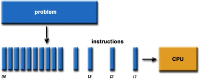
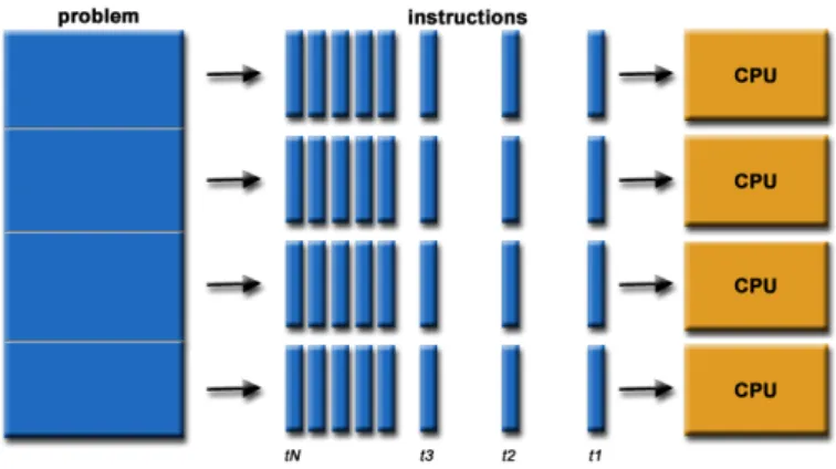
Figures 2.1 and 2.2 show a visual comparison between a standard sequential algorithm and a parallel algorithm running on a CPU with one core and a CPU with four cores respectively. Barney (2010) describes a useful example to help illustrate how a parallel algorithm relates to the real world. He states that parallel computing is simply an evolution of sequential computing that attempts to emulate what has always occurred in the real world with many complex, interrelated events happening at the same time while also in sequence.

Figure 2.1: A representation of a sequential algorithm on the CPU (Barney, 2010)

(13)

Figure 2.2: A representation of a parallel algorithm on multiple CPU (Barney, 2010)

2.1.1 Bernstein’s Conditions

There are many challenges in creating parallel algorithms. Data dependency issues are key in implementing parallel algorithms, as not fully comprehending them can severely affect the performance of an algorithm. In understanding the data dependencies of a sequential program, we can see whether it can be successfully parallelised or not.

Bernstein (1966) devised a set of conditions that must exist if two or more processes can be executed in parallel. We say thatIi is the set of all inputs for

a processPi. Similarly, Oi is the set of all outputs for a processPi.

When given two processes P1 and P2, they may execute in parallel if the

following rules are observed:

I1∩O2=∅ I2∩O1=∅ O1∩O2=∅

The rules defined by Bernstein (1966) state that two processes cannot ex-ecute in parallel unless they are flow independent (rule one), anti independent (rule two) and output independent (rule three).

Flow Dependent S1 precedes S2 where at minimum one output of S1 is an

input toS2

Anti Independent S1precedesS2where the output ofS2overlaps input toS1 Output Independent S1andS2write to the same unique output

For example, Algorithm 1 below cannot be implemented in parallel success-fully as there are issues with flow dependency. If we look at line four, we can see that this line cannot be executed before line three, as line four requires an input that depends on the outcome of line three.

(14)

However, Algorithm 2 is an example of a program that may be implemented in parallel, as there are no dependencies between data and instruction. Each line is independent and does not depend on the outcome of any other line.

Algorithm 1 dependency(int i, int j) 1: int k;

2: int l; 3: k = i * j; 4: l = 3 * k;

Algorithm 2 noDependency(int i, int j) 1: int k; 2: int l; 3: int m; 4: k = i * j; 5: l = 3 * j; 6: m = i + j;

2.1.2 Common Problems with Parallel Programming

Often, when creating parallel algorithms, desired tasks are split into threads whose purpose is to solve some task in parallel with other threads. Often, multiple threads will want to read, and modify a common variable in order to perform some task. This can lead to a serious problem known as a race condition. Race conditions occur when separate threads both depend on a shared state. Without proper management, the threads can hold incorrect data or process incorrect data that has not been updated correctly by a different thread (Netzer et al., 1992).

Consider Algorithm 3 that helps to clarify race conditions. Ti refers to a

resident thread of the parallel algorithm. Likewise,Ti refers to a register.

Algorithm 3 raceCondition() 1: int i = 0 2: T1 reads i intoR1 3: T2 reads i intoR2 4: T1 i = i + 1 (inR1) 5: T2 i = i + 1 (inR2)

6: T1 writesR1 back to memory

7: T2 writesR2 back to memory

In Algorithm 3, the result ini at the end of the algorithm is 1. However, the expected result is 2. To avoid this common problem, mutual exclusion must be provided by using a lock. The lock will allow a thread to assume control of a variable (in this case,i) and therefore stop any other thread from reading and/or writing to it until the controlling thread has released the lock.

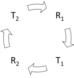
In utilising locks to solve race conditions, another serious problem is intro-duced. Deadlocks occur when two or more threads are waiting for the other(s)

(15)

to finish and neither of them ever do (Silberschatz et al., 2006). For example, imagine two threads (Tx) and two printers (Rx). Now, imagine each thread

requesting the other’s printer. This situation will cause a deadlock as the print-ers have not yet been released by the original threads. E.g. T1 is in control

of R1, but is also requesting R2. However, T2 currently controls R2; causing

a deadlock. This form of deadlock is known as circular deadlock, or a circular chain, and can be seen in Figure 2.3.

R

₁

T

₁

R

₂

T

₂

(16)

2.1.3 Flynn’s Taxonomy

When looking at the world of parallel computing, there are several ways in which you can classify a parallel computing machine. These classes could be based on the hardware architecture of the machine. For example, Flynn (1972) presents a method of classifying a parallel computing machine based on its hardware architecture, and therefore, programmability.

Flynn’s classification is based on two separate dimensions, Instruction and Data. Furthermore, these dimensions are split into two states, Single or Multi-ple. This leads to four possible classifications that form Flynn’s Taxonomy and can be seen in Table 2.1.

Single Instruction Multiple Instruction

Single Data SISD MISD

Multiple Data SIMD MIMD

Table 2.1: Flynn’s Taxonomy

As we will see in Section 2.4, the GPU used for this project is a Single Instruction, Multiple Data (SIMD) processor, capable of performing thousands of identical instructions on any number of pieces of data.

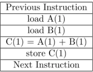
Single Instruction, Single Data (SISD)

Only a Single Instruction is being executed by the CPU during any given clock cycle.

Only a Single Data is being used as input for the current instruction during any given clock cycle.

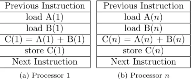
“Represents most conventional computing equipment available today” (Flynn, 1972). Previous Instruction load A(1) load B(1) C(1) = A(1) + B(1) store C(1) Next Instruction

Table 2.2: Single Instruction, Single Data

Single Instruction, Multiple Data (SIMD)

Only a Single Instruction is being executed by the CPU during any given clock cycle.

Multiple Datacan be used by each processor to allow for multiple inputs.

Best suited for systems with multiple streams of data, with a single in-struction. E.g. a modern GPU.

(17)

Previous Instruction load A(1) load B(1) C(1) = A(1) + B(1) store C(1) Next Instruction (a) Processor 1 Previous Instruction load A(n) load B(n) C(n) = A(n) + B(n) store C(n) Next Instruction (b) Processorn

Table 2.3: Single Instruction, Multiple Data

Multiple Instruction, Single Data (MISD)

Multiple Instructionsare being executed by each processor during any given clock cycle.

Only aSingle Datais used by each processor for input in any given clock cycle. Previous Instruction load A(1) load B(1) C(1) = A(1) + 1 store C(1) Next Instruction (a) Processor 1 Previous Instruction load A(1) load B(1) C(1) = A(1) + 1 store C(1) Next Instruction (b) Processorn

Table 2.4: Multiple Instruction, Single Data

Multiple Instruction, Multiple Data (MIMD)

Multiple Instructionsare being executed by each processor during any given clock cycle.

Multiple Datacan be used by each processor to allow for multiple inputs.

Execution on a MIMD can be either synchronous or asynchronous.

The most common form of parallel computer.

The majority of the world’s super computers follow the MIMD architec-ture.

(18)

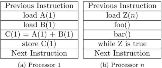
Previous Instruction load A(1) load B(1) C(1) = A(1) + B(1) store C(1) Next Instruction (a) Processor 1 Previous Instruction load Z(n) foo() bar() while Z is true Next Instruction (b) Processorn

(19)

2.2 GPGPU

In recent years, the advent of GPGPU has popularised the use of parallel com-puting on the GPU in achieving significant performance gains on a relatively cheap hardware device. GPGPU is a method of using the GPU to perform com-putations that would usually be executed by the CPU, rather than performing calculations to handle computer graphics, as is their traditional use. When the GPU is used for GPGPU, it can be viewed as a coprocessor to the CPU, offloading complex tasks that the GPU can tackle in parallel.

GPGPU provides an extremely cost effective alternative for parallel algo-rithms that would normally be exclusive to supercomputers, with a low-end CUDA enabled GPU costing approximately£25 compared to a super computer such as IBM’s Blue Gene system at$1.3million.

Multiple GPUs in a single system can be utilised for a single problem, of-ten increasing the performance of parallel applications. This project does not utilise multiple GPU however. The applications of GPGPU are far reaching and include some of the following:

Graph Theory.

Ray Tracing.

Matrix and/or Vector Operations.

Signal Processing.

Image Processing.

Speech Recognition.

Physics Simulations.

Medical Computation.

Multiple GPGPU APIs exist to utilise the GPU for parallel computing. Pop-ular APIs include NVIDIAs CUDA, OpenCL Khronos (2011) and DirectX’s DirectCompute platform (Microsoft, 2012). This research focuses solely on NVIDIAs CUDA API. Each have their advantages and disadvantages, but all provide a solid parallel computing API to utilise the powerful hardware of mod-ern GPU.

Modern graphics cards have a specialised hardware architecture that can be represented as a parallel computer. Unlike traditional graphics cards, GPUs such as NVIDIAs 580GTX are equipped with 16 multiprocessors, each with 32 cores, providing an impressive 512 cores. Each core has access to a global bank of memory, much like the Random Access Memory (RAM) on a PC, as well as a block of shared memory per multiprocessor which provides fast storage that can be used to share data between parallel processes. The potential of GPGPU is extremely great, given this unique hardware architecture that can provide great performance benefits to algorithms at a relatively low cost.

(20)

2.3 What is CUDA?

CUDA is a parallel computing solution developed by NVIDIA, encompassing both a software and hardware architecture for using an NVIDIA GPU as a par-allel computing device without the need for a graphics API. CUDA is available for all NVIDIA GPU following (and including) their G80 series of GPUs.

The CUDA API is an extension of the C programming language, providing programmers with a set of tools to create parallel algorithms. By providing the API in C, CUDA gives many programmers who already know C to quickly pick up their tools and begin creating CUDA applications.

CUDA enabled GPUs now have an install base of at least 100 million units (NVIDIA, 2009). Clearly, from this number, parallel algorithms utilising CUDA can be distributed easily to the mass market with a large number of machines supporting the technology, making CUDA an ideal candidate to boost the per-formance of a wide range of applications, both academically and commercially, examples of which are given in Section 2.2.

As a parallel computing platform, CUDA is designed to run thousands of threads at the same time, each thread executing the same code, but acting on multiple pieces of data, usually chosen programmatically to ensure that each thread works on a different pieces of unique data. Using this method, applica-tions can be executed on the GPU, rather than the CPU as described above.

The CUDA API provides both high and low level APIs to suit the program-mers needs. The lower level API provides a greater level of granularity and closeness to the underlying hardware, but decreases the readability and main-tainability of CUDA code. These APIs are known as the runtime and driver APIs, respectively. In older versions of CUDA, the driver API provided a greater level of detail in querying the GPU memory, in providing more information than the runtime API. However, large strides have been made in the latest CUDA re-leases, both in API usability, and CUDA compiler performance. The two APIs are mutually exclusive however, and their use must never overlap.

Despite providing greater control, the lower level driver API does not provide a performance increase over runtime code, and should simply be used if a greater amount of control over the GPU is required. Older versions of CUDA provided an emulator, so that CUDA may be programmed without the presence of a CUDA GPU. Emulation was not supported by the driver API, and the emulation program was deprecated with CUDA 3.0.

Since its inception, there has been strong evidence showing that parallel algorithms on the GPU can greatly improve the performance of classic problems when compared to their sequential (CPU) equivalents, providing a justification for research in this area.

(21)

2.4 CUDA Hardware Model

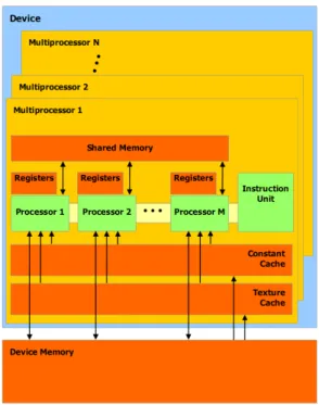
The architecture of a CUDA enabled GPU can be represented as a massive SIMD processor, examined in further detail in Section 2.1.3. A CUDA device consists of a number of multiprocessors, each with an identical number of pro-cessors (cores). Key to the architecture of CUDA devices is the different types of memory available, and their layout. Or, in other words, CUDAs memory hierarchy.

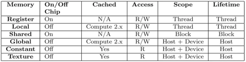
Table 2.6 gives a brief overview of the differing memory types, their access types, scope and locality. Additionally, Figure 2.4 shows these different types of memory that form CUDAs memory hierarchy and how they interact with the CUDA architecture on a higher level.

Memory On/Off Chip

Cached Access Scope Lifetime Register On N/A R/W Thread Thread

Local Off Compute 2.x R/W Thread Thread

Shared On N/A R/W Block Block

Global Off Compute 2.x R/W Host + Device Host

Constant Off Yes R Host + Device Host

Texture Off Yes R Host + Device Host

Table 2.6: Device Memory Features (NVIDIA, 2012)

Firstly and perhaps most importantly is shared memory. Shared memory is located directly on-chip with the multiprocessors, providing extremely fast read and write times to and from the processor. In utilising shared memory, an impressive performance gain of over 100x can be gained over global memory (NVIDIA, 2011a).

When possible, the greatest amount of data should be moved from device memory into shared memory to try and squeeze as much performance out of CUDA as possible. Once data is in shared memory, computations can be per-formed there before writing the results back to device memory and thus, re-ducing the effects of latency between the multiprocessors and device memory. Latency simply describes the delay in clock cycles between some action being requested, and the action completing.

Unfortunately, shared memory is very small in comparison to the other mem-ory types in CUDA. Older compute devices had just 16kb per multiprocessor to leverage. Newer compute devices however are graced with an additional 16kb, totalling 32kb per multiprocessor. Using shared memory wherever pos-sible in CUDA code is clearly very beneficial from a performance standpoint when utilised correctly, but the programmer should be wary of the memory constraints that go hand-in-hand with shared memory.

As well as shared memory, registers are located on-chip providing extremely quick access for local variables stored in CUDA code. The use of too many registers, increasing register pressure, can have a negative effect on system per-formance and is explained in more detail in Section 2.6.

As we can see in Figure 2.4, texture and constant caches are provided on top of shared memory, also located on-chip. Cache memory is read only, and must be populated with data before CUDA code is executed. This can be performed with one of the many memory allocation features provided by the CUDA driver and runtime APIs. Whilst not as fast as shared memory, they

(22)

provide a greater amount of storage, and are significantly faster than device memory (global memory).

Device memory, (also known as global memory or Dynamic Random Access Memory (DRAM)) is available to all multiprocessors and their cores, effectively acting as the GPUs RAM. Device memory offers by far the greatest amount of storage capacity on the GPU but also suffers from being the slowest of all forms of memory. Device memory takes several clock cycles to both read and write data to and from the multiprocessors. It is often necessary to use device memory, due to its sheer capacity, so its speed must be kept in mind at all times to ensure the greatest performance benefits when programming for CUDA.

Figure 2.4: CUDA Hardware Model, Demonstrating Memory Hierarchy and Overall Hardware Architecture of CUDA GPUs (NVIDIA, 2009)

Fundamentally, understanding the benefits and drawbacks of these contrast-ing memory types is important and can greatly affect the performance of code. In knowing which storage type to use before creating a CUDA application, we can speed-up our applications as much as possible.

When programming for CUDA, it is important to take into consideration the time taken to physically move data between the host and the device. Minimising data transfer between host and device is important because those transfers are subject to much lower bandwidth than when moving data internally on the device (NVIDIA, 2011a). In some cases, it may be beneficial to just compute the data you need on the device, rather than copying it from host memory to device memory. Due to the high bandwidth, low latency of shared memory, it is always beneficial to use it wherever possible. Either by copying data from device memory to shared, and performing calculations there, or by simply computing the data required directly into shared memory (NVIDIA, 2011a).

(23)

2.4.1 Coalesced Memory Access

“Perhaps the single most important performance consideration in programming for the CUDA architecture is coalescing global memory accesses” (NVIDIA, 2011a).

Dehne and Yogaratnam (2010) state that the goal of coalescing memory ac-cess is to combine multiple global memory acac-cess requests, by multiple threads, concurrently, into a single memory transaction for an independent portion of memory. The benefits of using this technique are vast, greatly improving the performance of the application. Using coalesced memory access can be a diffi-cult task to master, as the GPU hardware support for the system has changed quite significantly with each version of CUDA.

Early versions of CUDA (1.0/1.1) required that the kernel explicitly align memory access patterns so that each thread had to access consecutive memory blocks that related to the order of the threads. Kernels are explained in greater detail in Section 2.5. Imagine four threads, T0 to T3. To achieve coalesced

memory access, each thread must access memory locations A0 to A3 where A0 < A1 < A2 < A3 and are in a block of contiguous memory (Dehne and

Yogaratnam, 2010). The memory accesses by these threads are coalesced using a half-warp (explained a little further on) of threads, where a full warp consists of thirty two threads. In this way, sixteen thirty two bit reads are coalesced into one sixty four byte memory access. As noted by Dehne and Yogaratnam (2010), this method of memory coalescing is really quite inflexible and rather complicated to implement successfully.

With the release of CUDA 1.2, the rules for coalesced memory access were relaxed, allowing for easier, and more successful use of the system (NVIDIA, 2011b). With CUDA 1.2 and above, if sixteen data accesses fit into a thirty two byte memory segment, then a single memory access of thirty two bytes is performed. If however, those sixteen accesses do not fit into a thirty two byte segment, but do fit into a sixty four byte segment, a sixty four byte segment is performed instead.

If the data stored in global memory does not map well for coalescing, it can be beneficial to pad your data so that it may match the coalesced access patterns. Padding data simply means to add extra data that has no meaning in order to achieve some storage constraint. In that way, you can still benefit from the performance improvement of coalesced access. This is only possible however, if you have enough free memory that you can waste with data padding (NVIDIA, 2011b). Clearly, using this coalesced system allows for a significant performance improvement by allowing multiple pieces of data to be accessed in parallel, rather than sequentially.

(24)

2.5 CUDA Software Model

As explained in Section 2.3, two APIs are provided in order that CUDA might be programmed. Both APIs allow programmers to write special functions known as kernels that will be executed on the GPU. These kernels are structured in the same way as normal C functions, but are provided with additional intrinsics such asthreadIdxthat allow the executing thread to access information about itself. In this case, a 3-Dimensional vector (threadIDx) that holds the current thread’s address. Each component of the vector represents the threads x, y, andz co-ordiantes inside the thread block (explained below). This information can be used in a number of ways; most commonly in determining what data the thread should operate on.

In order to create a CUDA application, it is not necessary to understand the underlying hardware architecture, as it is hidden from the programmer. While a programmer does not need to understand the hardware architecture, it is extremely beneficial in being able to gain the most out of CUDA. By understanding the hardware architecture, as well as the intricate details of how CUDA threads operate and interact, the programmer can tailor his or her kernels to obtain the best performance possible from the code in utilising the many memory types and features of the CUDA architecture.

Instead of seeing the CUDA architecture when programming, threads are seen as being organised into blocks. Blocks are a convenient structure to think about threads in. A block is simply a 1, 2, or 3-Dimensional structure in which threads reside. In this way, groups of threads can easily be partitioned, allowing the programmer to easily decide how and where blocks should operate on data, and how shared memory should be utilised. Each thread is executed following the Single Program, Multiple Data (SPMD) model (see NVIDIA (2012)).

A programmer can define how many threads are executed for each kernel that is written. Taking the NVIDIA 8800GTX as an example, the programmer can define no more than 512 threads per block. Blocks can also be ordered into grids, with each grid holding at most 232_{blocks. Therefore, 2}41_{total threads can}

be executed per kernel. CUDA handles the assignment of threads and blocks to multiprocessors as well as other tasks including thread scheduling by utilising its GigaThread technology (see NVIDIA (2011b)).

The way in which threads are scheduled on the GPU differs greatly from the CPU. Whilst one might say that threads execute independently on the CPU, CUDA threads are scheduled in groups. These groups, known as warps, execute following the Single Instruction Multiple Thread (SIMT) model as described in Section 2.1.3. The minimum number of threads per warp is 32, with each thread inside the warp executing exactly the same instruction. Therefore, if the code being executed by the warp contains branches, each branch is expanded by filling in with null values where appropriate. Clearly, avoiding branches is critical as the performance of algorithms containing branches degrade as thread execution time is increased by expanding both branches.

CUDA provides functions that allow threads to be synchronised within a block. This synchronisation process acts as a barrier within the kernel which forces all threads in a block to hang until every thread in the block has reached the barrier. Blocks cannot be synchronised within a grid. Threads can be addressed using either a 1, 2, or 3-Dimensional index. Likewise, blocks may be addressed by a 1, 2, or 3-Dimensional index. CUDA provides thread and block

(25)

ID variables which can be used in a variety of ways to ensure that the threads in a kernel are performing the correct tasks on the correct piece or pieces of data. A very important aspect of a block, is that threads within a block can communicate via the GPU shared memory. This is the only form of thread communication available with CUDA. The GPU automatically schedules where and how blocks should be executed on the device. Blocks are always contained to one core, i.e. a block and its threads can never be split between different cores. This restriction ensures that each thread in the block can communicate via shared memory as shared memory is located on-chip (as discussed in Sec-tion 2.4). Organising threads and the data allocated to shared memory is often a complex task, with additional issues such as avoiding bank conflicts.

Bank conflicts occur where one block’s shared memory data overlaps an-other’s. Bank conflicts are discussed in more detail in Section 2.8. Evidently, utilising shared memory is highly beneficial but requires skill to accomplish it successfully. As mentioned previously, the programmer specifies the number of threads that are used for each kernel. The programmer can also specify the block size that is to be used for each kernel. A kernel can also be executed multiple times with differing thread and block sizes for each execution to create the desired results.

CUDA refers to the GPU as the device, whereas the CPU is the host. Ex-ecuting a kernel does not stop the host from exEx-ecuting it’s own code, allowing both device and host code to run simultaneously. This feature was only intro-duced in a recent version of CUDA however, and kernel calls used to be blocking. Having blocking code means that the CPU would not be able to continue the CPU section of a CUDA program until the kernel returned control to the host. If the host wishes to access device memory whilst a kernel is executing, it is necessary for the kernel to finish its execution. Therefore, the host code is blocked until kernel execution finishes, at which point the host may proceed. As of CUDA compute version 1.1 and above, asynchronous memory access is sup-ported whilst a kernel is executing, allowing host code to access device memory during kernel execution. This feature can be useful in certain problem domains, but for this project, its use is limited at best.

If the programmer wishes, multiple kernels can be executed asynchronously, allowing multiple differing tasks to be completed at once. In this regard, the kernels must be carefully written to ensure that enough memory is available for each kernel and that performance isn’t harmed by executing more than one kernel at any one time.

(26)

2.6 Occupancy

CUDA executes instructions sequentially within a thread block, so executing a warp whilst another is paused or blocked is the only way in which CUDA can hide latencies and attempt to keep the GPU busy. CUDA defines a metric, occupancy, that allows determination of how effectively the GPU is being kept busy by CUDA (NVIDIA, 2012).

NVIDIA define occupancy as the “ratio of the number of active warps per multiprocessor to the maximum number of possible active warps” (NVIDIA, 2012). Having a low occupancy can interfere with the ability of CUDA to hide the performance issues related to memory latency which in turn results in a decrease in performance of CUDA code. Conversely, having a high occu-pancy rating does not always equal a higher performance rating of CUDA code. NVIDIA (2012) state that there is a point in which additional occupancy does not improve CUDAs performance.

Register availability is one of the major factors that can affect the occupancy of CUDA code. Kernels use registers to enable threads to store local variables in extremely efficient memory, allowing for low latency access by the thread. The number of registers available are limited, making them a scarce resource for thread blocks. They must be shared between all threads and blocks that reside on a single multiprocessor. As registers are allocated by the CUDA compiler all at one time, the number of threads that may reside on a multiprocessor is reduced as there are a limited number of registers. This leads to a lower occupancy rating due to the simple fact that fewer threads can be allocated to a multiprocessor when lots of registers need to be allocated to a thread block.

In calculating occupancy, the number of registers used by a thread is very important. CUDA devices with compute capability 1.0/1.1 have 8,192 registers per multiprocessor and can also have at most 768 threads resident on a multi-processor at any one time (NVIDIA, 2012). With these statistics, each thread would have to use at most 10 registers to achieve 100% occupancy.

The exact nature of the relationship between register use and occupancy can be difficult to determine (NVIDIA, 2012). Due to the fact that register alloca-tion differs slightly between different compute versions of CUDA devices, and the fact that a multiprocessor’s shared memory is also partitioned between dif-fering thread blocks, exact occupancy calculation is a difficult task. To combat this, NVIDIA provide CUDA developers with a spreadsheet in which critical data about CUDA kernels can be entered to provide an occupancy rating for the code. Additionally, NVIDIA provide a profiling tool that allows the CUDA code to be executed and monitored to calculate an occupancy rating.

(27)

2.7 Thread and Block Heuristics

When choosing the number of threads per block, a multiple of 32 threads is recommended by NVIDIA as to ensure “optimal computing efficiency” and fa-cilitate coalescing (NVIDIA, 2012). By ensuring the correct parameters for the number of threads per thread block, the balance between the latency of a CUDA application and resource utilisation can be found.

Occupancy and latency hiding depend on the number of active warps per multiprocessor which in turn depends on the register and shared memory con-straints set by the compute capability of the GPU. To balance occupancy with resource allocation, the correct execution parameters should be chosen (NVIDIA, 2012).

Kernels should be designed to try and keep the GPU as active as possible, ensuring that there is as little idle time as possible whilst a kernel is executing. A simple way of doing this is to ensure that the number of blocks specified is greater than the number of multiprocessors on the GPU. Different GPUs have contrasting numbers of multiprocessors however, which is important to keep in mind. In this way, each multiprocessor has at least one thread block to execute. Increasing the number of thread blocks so that each multiprocessor is assigned multiple thread blocks by the compiler is important. In doing this, if a thread block is forced to wait by a syncthreads() command, execution can be switched to another thread block, thus helping to keep the GPU busy at all times. NVIDIA recommend using thousands of thread blocks per kernel launch to ensure scalability with future GPUs (NVIDIA, 2011a).

Clearly, occupancy is not just determined by block size as many blocks may be present on a single multiprocessor at any one time. NVIDIA (2012) give the example that having a block size of 512 threads may result in occupancy of 66% as the maximum number of threads is 768. Therefore, only one active block would reside on a multiprocessor. However, a smaller block of 256 threads could result in 100% occupancy as there would be three active blocks on the multiprocessor.

Selecting the correct block size is important for the reasons described above, but there are several factors in choosing the block size, depending on the task at hand. Currently, experimenting with block sizes is needed to obtain the best performance, but NVIDIA (2012) provide the following rules that should be followed to ensure block and thread heuristics are set correctly.

Threads per block should be a multiple of warp size to avoid wasting computation, and to facilitate coalescing.

At least 64 threads per block should be used.

Between 128 and 256 threads per block is a better choice however. This provides a good base range for initial experimentation of different block sizes.

If latency is an issue, use smaller thread blocks rather than one large one. This is especially useful if syncthreads() is frequently used.

(28)

2.8 Bank Conflicts

As we know from Sections 2.4 and 2.5, shared memory has a much higher band-width and lower latency than global memory. This is not the case however where bank conflicts occur. Shared memory is divided into equally sized block (banks) that are accessible simultaneously by threads resident on a single mul-tiprocessor. “Therefore, any memory load or store ofn addresses that spansn

distinct memory banks can be serviced simultaneously” (NVIDIA, 2012). As a result, thread blocks can achieve a bandwidth that is n times as great as the bandwidth capabilities of a single bank on its own.

If however, there are several memory addresses in a request that map to the same bank of shared memory, a bank conflict occurs and the access to the bank is serialised, impacting the performance of the kernel. In an attempt to reduce the effects of bank conflicts, the GPU will attempt to split each memory request that will result in a bank conflict into as many requests as necessary, so as to avoid conflicts, thus decreasing the bandwidth of the memory access.

(29)

2.9 Chapter Summary

In this chapter, a general overview of parallel computing was discussed, as well as an in-depth look at GPGPU and more specifically, CUDA.

We have seen how Bernstein’s Conditions can be used to identify whether an algorithm or process can be implemented in parallel by understanding what inherent dependencies are present in the process. In order that a process might be implemented in parallel, it must be flow independent, anti independent, and output independent.

Many new and interesting problems may present themselves in parallel com-puting. We have seen how race conditions can drastically effect how a program operates, in potentially resulting in incorrect data being read/written. This problem can lead to deadlock, whereby different threads end up waiting for other threads to finish a task, and therefore stall due to neither of them ever finishing.

Flynn’s Taxonomy is an important framework for identifying how a parallel computer might be implemented. Flynn (1972) presents three classifications, SIMD, MISD, MIMD for identifying a parallel computer, and how it operates. As well as one classification, SISD, which identifies a traditional sequential com-puter. These classifications were later used in identifying how a CUDA GPU operates.

On looking at the GPGPU space, we have seen many useful applications of GPGPU, as well as several high profile APIs available for utilising the technol-ogy. CUDA was identified as a GPGPU API, as well as the one that will be utilised for this thesis. We have seen in great detail how the CUDA hardware and software models are composed, providing a parallel platform in which many thousands of resident threads may be executed in order to improve the perfor-mance of a subject problem. Technicalities of CUDA were presented, such as bank conflicts, and deciding on what memory type(s) should be utilised when implementing applications for CUDA.

(30)

Chapter 3

Introduction to the

All-Pairs Shortest Path

Problem

Graphs are an extremely common data structure in the field of computer science. There are many different problems that can and are represented as graphs, and algorithms to manipulate them are very important and widely used. This section looks at graph algorithms in terms of the APSP problem.

3.1 What is the APSP Problem?

Imagine trying to find the shortest distance between all pairs of cities in an atlas. This problem can be solved using an APSP algorithm by representing the cities and roads between them as vertices and edges respectively. More formally, given a directed, weighted graphG= (V, E), we wish to find for every pair of vertices

u, v∈V, a least weight (shortest) path fromutov, whose weight is the sum of all edges in the path (Cormen et al., 2001). |V|denotes the number of vertices in the set and|E|similarly denoting the number of edges inG.

The problem can be solved by running an algorithm that solves the Single-Source Shortest Path (SSSP) problem by running it on every vertex in G. A popular way of solving the problem using this means is using Dijkstra’s SSSP algorithm. The edges’ weights must be non-negative in order to use Dijkstra’s algorithm for APSP. If negative edge weights are allowed, the slower Bellman-Ford algorithm must be used (Cormen et al., 2001). Where negative cycles are allowed, there is no shortest path as the traversal of such a cycle continually reduces the cost of the path. An algorithm using this approach is described in Section 4.3. A “true” APSP algorithm does not take this approach however. The following algorithms are expanded on in the following sections.

(31)

3.2 Sequential Algorithms

3.2.1 The Floyd-Warshall APSP Algorithm (Floyd, 1962)

The majority of CUDA algorithms described in Chapter 4 are originally based upon this algorithm so it is important to fully understand the theory behind it, and how it is implemented correctly.

The Floyd-Warshall algorithm utilises a dynamic programming technique and runs in O(n3_{) time (Cormen et al., 2001). The algorithm operates on a}

directed graphG= (V, E) with non-negative edge weights. The algorithm can however operate if required with negative edge weights. If a cycle was to exist with total negative weight, the Floyd-Warshall algorithm can be used to detect them. Initially, all path lengths are 0. If negative cycles exist between two vertices, the path length between those two vertices will be negative.

Using the observations in Cormen et al. (2001), for any pair of vertices u

and v, observe all paths from uto v where the intermediate vertices are from some subset of V {1,2, ..., k} for anyk. Additionally, let pbe a path amongst

uandv that is of a minimum weight.

Floyd-Warshall uses the relationship between pand all shortest paths be-tween bothuandvwith all of the intermediate vertices in the set{1,2, ..., k−1}. Depending on whetherkis an intermediate vertex or not, one of two things can happen. Wherekis not an intermediate vertex ofp, all of the intermediate ver-tices inpmust be in{1,2, ..., k−1}. To that end, the least cost path between

uandv will also be in the set{1,2, ..., k}.

However, if k is an intermediate vertex ofp, pcan be split into two paths such thatp1 is that path from uto k and the pathp2 is fromk to v. Ask is

no longer an intermediate vertex, p1 is the shortest path fromutok where all

intermediate vertices are in{1,2, ..., k−1}andp2is the shortest path fromkto v where all intermediate vertices are in{1,2, ..., k−1}. This observation holds in that a subpath of a shortest path is in itself, a shortest path, as described by Cormen et al. (2001).

Algorithm 4 Floyd-Warshall 1: fork= 0to n

2: foru = 0 ton 3: forv = 0ton

4: graph[u][v] = min(graph[u][v], graph[u][k] + graph[k][v]) 5: end

6: end

7: end

Algorithm 4 demonstrates how simple the Floyd-Warshall algorithm is to implement on the CPU. The computations can be done in place, meaning that the graph does not need to be copied and therefore, keeping the same amount of memory. This basic construct is used and modified by the majority of the following CUDA algorithms, and is a classic solution to the APSP problem.

(32)

3.2.2 Dijkstra’s Algorithm (Dijkstra, 1959)

As mentioned in Section 3.1, Dijkstra’s algorithm, which solves the SSSP prob-lem, can be used to solve APSP by repeating the algorithm on every vertex in a graph. Harish and Narayanan (2007) describe a CUDA algorithm based on Dijkstra’s algorithm which is detailed in Section 4.3. A good implementation of Dijkstra’s algorithm has a lower running time than that of the Bellman-Ford algorithm described in Section 3.2.3.

Dijkstra’s algorithm maintains a setSof vertices whose shortest path weights from the source vertexshave already been determined. The algorithm repeat-edly selects a vertex v ∈ V −S with “the minimum shortest path estimate” and then adds uto S, finally relaxing the edges that leaveu. To improve on the Bellman-Ford algorithm, a minimum-priority queue Qis used. The origi-nal algorithmic description by Dijkstra does not use a minimum-priority queue (Dijkstra, 1959).

Algorithm 5 Pseudo Code for Dijkstra’s Algorithm (Cormen et al., 2001) 1: S ∅

2: QV

3: while Q6=∅

4: do uEXTRACT-MIN(Q) 5: S S ∪ {u}

6: foreach vertexv∈adj[u] 7: doRELAX(u, v, w)

We can see from Algorithm 5 that the loop invariant on line three will be true at the start of the algorithm. As the algorithm proceeds through the loop, a vertexuis extracted fromQand immediately added toS. This process maintains the invariant, and from it, we can see that the algorithm loops exactly

|V|times. This holds as each vertex is removed fromQand added toSexactly once each. As edges are relaxed on lines four to seven, the path cost estimate is updated if the shortest path can be improved by passing throughuto get to

v (Cormen et al., 2001).

Dijkstra’s algorithm uses a greedy approach in that it chooses the next closest or lightest vertex. Greedy algorithms are not always optimal but in Dijkstra’s case, this algorithm does present an optimal solution. A proof for this can be found in the work by Cormen et al. (2001).

Dijkstra’s algorithm gives us a running time of O(|E|+|V|log|V|) when implemented using a minimum-priority queue that is represented by a Fibonacci heap. With this method, each call to EXTRACT-MIN only takes O(log|V|) and each RELAX call takes justO(1) of which there are |E| calls. The Relax algorithm is explained in Section 3.2.3 and shown in Algorithm 7.

The running time of the algorithm changes when solving the APSP problem. As the algorithm is run |V| times for each vertex, the new running time is

(33)

3.2.3 The Bellman-Ford Algorithm (Bellman, 1958)

The Bellman-Ford algorithm solves the SSSP problem but like other SSSP al-gorithms, it can be used to solve APSP as well, by running on each vertex in

G. Unlike Dijkstra’s algorithm, the Bellman-Ford algorithm may operate on graphs with negative edge weightings and also has an asymptotic running time that is worse than Dijkstra’s. For that reason, the Bellman-Ford algorithm is usually used where negative edge weights may be present, as Dijkstra’s cannot operate on such a graph.

The algorithm will return a boolean variable that specifies whether the graph contains a negative weight cycle that may be reachable from the source vertex

s. If a cycle is found, the algorithm states that there is no solution and ceases execution. If however, there is no cycle, the shortest paths and their weights are calculated.

During the algorithm, all edges inGare relaxed (as shown in Algorithm 7). The Relax algorithm looks at whether the path tovcan be improved if the path goes through u. If so, bothd[v] andπ[v] are updated. This continues until the shortest paths have been calculated. Once completed, the algorithm will return

trueif, and only if, no negative weight cycles are detected.

Algorithm 6 Pseudo Code for the Bellman-Ford Algorithm (Cormen et al., 2001)

1: INITIALISE SINGLE SOURCE(G, s) 2: fori1 to|V[G]| −1

3: do foreach edge (u, v)∈E[G] 4: doRELAX(u, v, w) 5: foreach edge(u, v)∈E[G] 6: do if d[v]> d[u] +w(u, v)

7: then returnFALSE

8: returnTRUE

The Bellman-Ford algorithm runs inO(|V||E|) time. Line one in Algorithm 6 takes Θ(|V|) time. Following that, each of the edge relaxations in line four take Θ(|E|) time and the for loop over lines five - seven takeO(|E|) time. Thus, the running time results inO(|V||E|).

Algorithm 7 Pseudo Code for the Relax Algorithm (Cormen et al., 2001) 1: RELAX(u,v,w)

2: if d[v]> d[u] +w(u, v)

3: thend[v] d[u] +w(u, v) 4: π[v]u

(34)

3.2.4 Blocked Algorithm (Venkataraman et al., 2003)

The Blocked Algorithm by Venkataraman et al. (2003) was designed, and op-timised, with CPU cache in mind, rather than optimising for RAM, which was the standard at the time. In utilising cache, Venkataraman et al. (2003) can achieve a substantial speed-up over the standard Floyd-Warshall algorithm in solving the APSP problem.

The algorithm begins by partitioning the adjacency matrix into sub matrices of size B×B where B is known as the blocking factor. Usually, it is normal for B to divide wholly into |V|. The algorithm performs B iterations of line one in Algorithm 4 on each B×B block ofD before it proceeds to the nextB

iterations (Venkataraman et al., 2003).

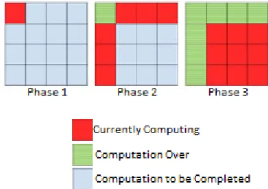
To increase understanding of the algorithm, Venkataraman et al. (2003) suggest thinking of each set of B iterations as being split into three separate phases. In phase 1 of the first iteration, Algorithm 4 is used to compute the elements within the sub matrix located at (0,0). As this set of iterations only accesses the elements within this block, Venkataraman et al. (2003) state that the sub matrix is called the self-dependent block. In the following code snippets we say thatk is 1≤k≤B.

In phase 2, a modified version of Algorithm 4 is used to compute the remain-ing sub matrices that are on the same row and column as the self-dependent block. For the sub matrices on the same row, the computation

Dk(i, j) =min{Dk−1(i, j), DB(i, k) +Dk−1(k, j)}

is used. Likewise, for the remaining sub matrices on the same column as the self-dependent block, the computation

Dk(i, j) =min{Dk−1(i, j), Dk−1(i, k) +DB(k, j)}

is used.

Finally, in phase 3, the remaining sub matrices are computed. Like phase 2, this computation is completed using a modified version of Algorithm 4:

Dk(i, j) =min{Dk−1(i, j), DB(i, k) +DB(k, j)}

Now that phase 3 is complete, the next round ofB iterations is computed by the Algorithm 8. This time however, the self-dependent block is located at (1,1). The process then repeats until B iterations of the algorithm have been performed. We are left with an algorithm that solves the APSP problem with the intention of improving running times when compared to the standard Floyd-Warshall algorithm (Algorithm 4).

(35)

Algorithm 8 Code for the Blocked Floyd-Warshall Algorithm (Venkataraman et al., 2003)

for(round = 1; round≤n / B; round ++)

for(k = (round - 1) * B + 1; k != round * B; k ++)

for(all i and j in block)

D[i][j] = min(D[i][j], D[i][k] + D[k][j]);

end end

do the remaining for all remaining blocks: phase 2 blocks

phase 3 blocks

for(k = (round - 1) * B + 1; k≤round * B; k ++)

for(all i and j in block)

D[i][j] = min(D[i][j], D[i][k] + D[k][j]);

end end end

(36)

Proving the Blocked Algorithms Correctness

We begin with a bit of notation. Suppose thatP1,P2 andP3are sets of paths

in G. Suppose that some path pis the concatenation of a path p2 in P2 with

a path p3 in P3; so, in particular, the last vertex of p2 must be equal to the

first vertex of p3. We say thatp2 is a prefix of p, with p3 the complementary suffix. Define P2·P3 as the set of paths in G having a prefix in P2 so that

the complementary suffix is inP3(note that we disallow walks, obtained in this

way, that are not paths).

The following definitions are needed for this section.

1. We denote byPc₍_{u, v}_{) the set of all paths from vertex}_u_{to vertex}_v _in_G

where the internal vertices come from{1,2, . . . , c}.

2. For any set of paths P, we denote by minP the minimum weight of the paths ofP or∞ifP is empty.

3. We define the n×n matrix Ac _{so that} _Ac₍_{u, v}_{) = min}_Pc₍_{u, v}_{); that}

is, Ac₍_{u, v}_{) is the value} _lc

u,v (see the previous section), with Ac(u, v) =

min{Ac−1(u, v), Ac−1(u, c) +Ac−1(c, v)}. Define

ϕ(P1, P2, P3) =P1∪(P2·P3).

Note that ifP1⊆P10,P2⊆P20 and P3⊆P30 then ϕ(P1, P2, P3)⊆ϕ(P10, P20, P30)

(we shall return to this fact later). Also, note that

Pc(u, v) =ϕ(Pc−1(u, v), Pc−1(u, c), Pc(c, v)),

or

P_x,yc (i, j) =ϕ(P_x,yc−1(i, j), P_x,zc−1(i, k), P_z,yc−1(k, j)) whereu=xb+i,v=yb+j andc=zb+k.

Suppose that we amend the recurrence within Floyd-Warshall slightly so that if u=xb+i,v=yb+j, c=zb+kand ¯c= (z+ 1)b(and so c≤c¯) then we define the following sets of paths:

_P˜0 x,y(i, j) =P 0 x,y(i, j) _P˜c z,z(i, j) =Pz,zc (i, j) _P˜c x,z(i, j) =ϕ( ˜Px,zc−1(i, j),P˜x,zc−1(i, k), Pz,zc¯ (k, j)),ifx6=z _P˜c

z,y(i, j) =ϕ( ˜Pz,yc−1(i, j), Pz,z¯c (i, k),P˜z,yc−1(k, j)),ify6=z

_P˜c

x,y(i, j) =ϕ( ˜Px,yc−1(i, j), Px,zc¯ (i, k), Pz,y¯c (k, j)),ifx6=z6=y

with ˜Ac

x,y(i, j) = min ˜Px,yc (i, j).

We now detail two inductions. Our first induction hypothesis is that no matter what the values of u and v, we have that the set of paths ˜Pc−1

x,y (i, j)

from u to v in G is such that all internal vertices on any path come from the set of vertices {1,2, . . . ,¯c}. The base case of the induction (when c = 0) holds by definition, and the construction above immediately yields that we must have that the set of paths ˜Pc

(37)

internal vertices on any path come from the set of vertices {1,2, . . . ,¯c}. Thus, in particular, ˜Pc

x,y(i, j)⊆Px,y¯c (i, j).

Suppose as our induction hypothesis that no matter what the values of u

andv, we have a set of paths ˜Pc−1

x,y (i, j) fromuto v inGsuch that all internal

vertices on any path come from the set of vertices {1,2, . . . ,¯c} and such that

Pc−1

x,y (i, j)⊆P˜x,yc−1(i, j). From the definitions above, we trivially have that every

path in ˜Pc

x,y(i, j) only has internal vertices from the vertex set {1,2, . . . ,¯c}.

Furthermore, we have the following:

ifx6=zthen

Px,zc (i, j) = ϕ(Px,zc−1(i, j), Px,zc−1(i, k), Pz,zc−1(k, j))

⊆ ϕ( ˜P_x,zc−1(i, j),P˜_x,zc−1(i, k), P_z,z¯c (k, j)) = P˜x,zc (i, j)

ify6=z then

P_z,yc (i, j) = ϕ(P_z,yc−1(i, j), P_z,zc−1(i, k), P_z,yc−1(k, j))

⊆ ϕ( ˜P_z,yc−1(i, j), P_z,zc¯ (i, k), P_z,yc−1(k, j)) = P˜_z,yc (i, j)

ifx6=z6=y then

P_x,yc (i, j) = ϕ(P_x,yc−1(i, j), P_x,zc−1(i, k), P_z,yc−1(k, j))

⊆ ϕ( ˜P_x,yc−1(i, j), P_x,zc¯ (i, k), P_z,y¯c (k, j)) = P˜_x,yc (i, j).

So, by induction, we have thatP_x,yc (i, j)⊆P˜_x,yc (i, j) no matter what the values ofuandv and for all valuescfrom {0,1, . . . , n}.

However, whenc = zb we also have that ˜Px,yc (i, j)⊆ Px,yc (i, j), and so for

suchc, ˜Px,yc (i, j) = Px,yc (i, j) with ˜Anx,y(i, j) =An(u, v). Consequently, we can

(38)

3.3 Chapter Summary

In this chapter, we have investigated the formulation of the APSP problem as well as several sequential solutions to the problem.

In identifying the APSP problem, we have seen that it is a way of finding the shortest path between every pair of vertices in a given weighted graphG. This can be solved by utilising specific APSP algorithms, or by performing algorithms that solve the SSSP problem on every vertex inG.

Several APSP algorithms are presented which will later be discussed in re-lation to CUDA algorithms. These CUDA algorithms are originally based the sequential algorithms presented in this chapter. We have seen a very popular APSP algorithm presented by Floyd (1962) which solves the problem in place in O(V3_{). Additionally, we have seen the classic SSSP algorithm presented by}

Dijkstra (1959) and how it can be utilised for the APSP problem. The Bellman-Ford algorithm is also an SSSP algorithm that can solve the APSP problem by executing it on every vertex in G. However, we have seen that the Bellman-Ford algorithm has the added benefit of working on graphs with negative edge weights, whereas Dijkstra’s algorithm does not have this capability. We have seen that Dijkstra’s algorithm has a better running time than Bellman-Ford and so should always be used unless there are negative edge weights.

Finally, a blocked CPU algorithm based on Floyd-Warshall’s APSP algo-rithm is observed, which provides an improved running time over the Floyd-Warshall algorithm. A proof of correctness is provided for this algorithm, as it is based on the well documented Floyd-Warshall algorithm, but forms the basis of a critical CUDA algorithm.

An understanding of these algorithms is critical in presenting CUDA imple-mentations of APSP algorithms, as many of them are based on these classic CPU algorithms.

(39)

Chapter 4

Implementation of APSP

Algorithms Using CUDA

4.1 Graph Representations with CUDA

GPU memory layout is optimised for rendering graphics and cannot support user-defined data structures efficiently (Harish et al., 2009). Whilst data struc-tures for use on the CPU have been studied extensively, the use of hash tables (Hyvonen et al., 2008) for example, that are efficient on the CPU, are not suit-able for the GPU (Harish et al., 2009).

Of the algorithms detailed in this chapter, two different graph representa-tions are used. These implementarepresenta-tions are described here, to provide a full understanding that may be used when describing the APSP algorithms. The way in which a graph to be searched is stored on the GPU is critically impor-tant. Trade-offs between time and memory constraints have to be considered when choosing the memory layout for a graph. LetG= (V, E) be a graph with the vertex setV and the edge setE. We will use this notation for the rest of the paper to denote the graphs that we will perform searches on for all APSP algorithms. In that way, we can maintain a coherent approach to the way in which we describe all algorithms.

4.1.1 Adjacency Lists

Traditional methods of storing graphs, such as using an adjacency matrix, pro-vide a constant time method, O(1), of determining whether there is an edge

e between two vertices,uand v, but compromises on memory usage,O(|V|2_).

For sparse graphs, adjacency matrices are largely wasteful, holding data where no edges exist in the graph.

Adjacency lists provide a method of storing graphs which requires vastly less memory than an adjacency matrix,O(|V|+|E|). An adjacency list achieves this low memory usage by only holding vital information. However, the drawback of using such a list is a more expensive lookup time to determine if there is an edge between two vertices O(|V|). Harish and Narayanan (2007) and Harish et al. (2009) describe the use of a compacted adjacency list represented in Figure 4.1. They argue that due to the variable nature of graphs (number of vertices and

(40)

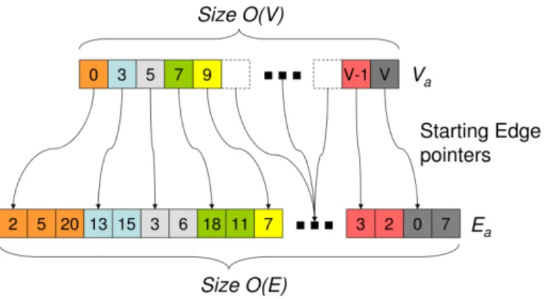
edges per graph), using an adjacency list representation may not be completely efficient on the GPU. Therefore, they use a modified version of an adjacency list, known as a compacted adjacency list where all of the information that would usually be stored in several lists, is compacted into a single, one dimensional array.

Figure 4.1: Graph Representation as a Compacted Adjacency List (Harish et al., 2009)

Demonstrating a compacted adjacency list, Figure 4.1 shows the vertex list (Va) and the edge list (Ea). The vertex list points to a starting index in Ea

which then represents the vertices incident to it. This method of storing an input graph is suitable for both undirected and directed graphs and can be expanded with a further array of equal size to|Ea|to represent edge weights (Wa). Using

several one dimensional arrays is suitable for use in CUDA as several blocks of contiguous memory can easily be allocated onto the GPU. When using a two dimensional array with CUDA, the compiler simply allocates a contiguous block of memory anyway, and automatically converts the two dimensional array into a one dimensional array, adding a hidden cost to running times.

4.1.2 Adjacency Matrices

Katz and Kider (2008) and Buluc et al. (2010) look at an alternative way of storing their graphs on the GPU, opting to use the standard adjacency matrix representation. Despite the downsides to using an adjacency matrix as described in section 4.1.1, this is an appropriate choice due to the way the computations are calculated in the relevant algorithms. Their implementations make use of shared memory which maps extremely well to the nature of an adjacency list.

Katz and Kider (2008) manage to store graphs with just over 11,000 vertices, occupying a considerable 1.015Gigabyte (109 _{bytes)s (GBs) of data. Using the}

compacted adjacency list, graphs of 10million vertices with a degree of six are possible on a GPU with just 768Megabyte (106_{bytes)s (MBs) of memory (Harish}

(41)

4.2 Mapping Threads to Vertices

It is often necessary to map each threadtto a vertexv such that eachthas one uniquev corresponding to it. When dealing with thousands of blocks, threads and vertices, it becomes convenient to have a common function to calculate this for us. To that end, we created a function that takes the current information about t, including its position in a thread block, as well as block and grid dimensions, to return an integer value that will assign t to v. As described in Section 2.5, CUDA provides multidimensional thread organisation as well as the necessary naming constructs to identify thread and block co-ordinates. Using threadID.x for example, will return that threads current xcoordinate. The same principle applies to thread blocks and grids, as well as y and z co-ordinates. The function listed in Algorithm 9 is used throughout this paper and will be referred to again several times as “obtainThreadID”.

Algorithm 9This Function is used by Algorithms that use the Graph Structure Described in Section 4.1.2

1: vertex = 0

2: vertex = vertex + threadIDX + (blockIDX * blockDimension.x) 3: vertex = vertex + (threadIDY + (blockIDY * blockDimension.y)) 4: vertex = vertex + blockDimension.x * gridDimension.x

All-Pairs Shortest Path Algorithms Using CUDA

Durham E-Theses

All-Pairs Shortest Path Algorithms Using CUDA

KEMP, JEREMY,MARK

All-Pairs Shortest Path Algorithms Using

CUDA

Jeremy M. Kemp

All-Pairs Shortest Path Algorithms Using

CUDA

Jeremy M. Kemp

Contents

List of Figures

List of Tables

Glossary

Copyright

Acknowledgements

Chapter 1

Introduction

1.1

Research Overview

1.2

Intended Outcomes

1.3

Thesis Overview

Chapter 2

Definitions

2.1

Parallel Computing

2.1.1

Bernstein’s Conditions

2.1.2

Common Problems with Parallel Programming

R

1

T

1

R

2

T

2

2.1.3

Flynn’s Taxonomy

2.2

GPGPU

2.3

What is CUDA?

2.4

CUDA Hardware Model

2.4.1

Coalesced Memory Access

2.5

CUDA Software Model

2.6

Occupancy

2.7

Thread and Block Heuristics

2.8

Bank Conflicts

2.9

Chapter Summary

Chapter 3

Introduction to the

All-Pairs Shortest Path

Problem

3.1

What is the APSP Problem?

3.2

Sequential Algorithms

3.2.1

The Floyd-Warshall APSP Algorithm (Floyd, 1962)

3.2.2

Dijkstra’s Algorithm (Dijkstra, 1959)

3.2.3

The Bellman-Ford Algorithm (Bellman, 1958)

3.2.4

Blocked Algorithm (Venkataraman et al., 2003)

3.3

Chapter Summary

Chapter 4

Implementation of APSP

₁

₁

₂

₂