Washington University in St. Louis
Washington University Open Scholarship
Engineering and Applied Science Theses &
Dissertations McKelvey School of Engineering
Spring 5-18-2018
Completing Cooperative Task by Utilizing
EEG-based Brain Computer Interface
Jongwoon Kim
Washington University in St. Louis
Follow this and additional works at:https://openscholarship.wustl.edu/eng_etds
Part of theEngineering Commons
This Thesis is brought to you for free and open access by the McKelvey School of Engineering at Washington University Open Scholarship. It has been accepted for inclusion in Engineering and Applied Science Theses & Dissertations by an authorized administrator of Washington University Open Scholarship. For more information, please [email protected].
Recommended Citation
Kim, Jongwoon, "Completing Cooperative Task by Utilizing EEG-based Brain Computer Interface" (2018).Engineering and Applied Science Theses & Dissertations. 344.
WASHINGTON UNIVERSITY IN ST. LOUIS School of Engineering and Applied Science Department of Electrical and Systems Engineering
Thesis Examination Committee:
ShiNung Ching, Chair Jason Trobaugh
Kevin Wise
Completing Cooperative Task by Utilizing EEG-based Brain Computer Interface by
Jongwoon Kim
A Thesis presented to the School of Engineering &
Applied Science of Washington University in partial fulfillment of the
requirements for the degree of Master of Science
May 2018 St. Louis, Missouri
ii
Table of Contents
List of Figures ... iii
List of Tables ... iv Acknowledgments... v ABSTRACT ... vii Chapter 1 Introduction ... 1 1.1 Motivation ... 1 1.2 EEG Signals ... 2 1.3 Frequency Bands ... 5 1.4 Apparatus ... 6 1.5 Objectives... 6
Chapter 2 Methods I: Spectral Analysis ... 9
2.1 Theories of Discrete Fourier Transform ... 9
2.2 Time-frequency Spectrograms ... 10
Chapter 3 Methods II: Feature Extraction and Classification ... 14
3.1 Classification ... 14
3.2 Weber Contrast ... 18
3.3 Information Transfer Rate ... 18
Chapter 4 Methods III: Data Acquisition and Experimentation ... 20
Chapter 5 Results ... 22
5.1 Spectrum and Spectrogram ... 22
5.2 Classification and Information Transfer Rate ... 28
5.3 Cooperative Task ... 32
Chapter 6 Discussion ... 34
6.1 Artifacts and Distortion ... 34
6.2 Signal Processing ... 40
Chapter 7 Conclusions ... 44
Chapter 8 References ... 46
iii
List of Figures
Figure 1: A closed loop block diagram of a BCI ... 1
Figure 2: Model of extracellular potential generated by a single action potential ... 3
Figure 3: A Diagram of the Cooperative Task... 8
Figure 4: A two-second segment of EEG signal obtained from the Muse headband and the DFT of the segment ... 10
Figure 5: A spectrogram of a linear chirp ... 11
Figure 6: DTFT of different windows in dB ... 12
Figure 7: Two datasets plotted with respect to features or variables, X1 and X2 ... 16
Figure 8: Linear discriminator using support vector machine ... 17
Figure 9: Segments of EEG signal while the subject is under relaxed and focused states ... 23
Figure 10: Spectrogram of the EEG signals while the subject was focused ... 25
Figure 11: Spectrogram of the EEG signals while the subject was relaxed ... 26
Figure 12: Spectrogram of the EEG signals while the subject was relaxed and focused for different intervals ... 27
Figure 13: Four features are plotted with respect to the number of samples. ... 29
Figure 14: The trajectory of the cursor driven by subject 4 and 5. ... 33
Figure 15: The weighted features and the threshold of subject 4 and 5 with respect to time. ... 33
Figure 16: A segment of the EEG signal while the subject is focused. ... 35
Figure 17: Spectrogram was created with different type of windows ... 36
Figure 18: A stripe of the Artifact seen in the spectrogram. ... 38
Figure 19: Segment of the time domain signal ... 39
Figure 20: Different windows ... 40
iv
List of Tables
Table 1: Information of each subject ... 21
Table 2: The weights on each feature for each subject implemented with LDA. ... 30
Table 3: The weights on each feature for each subject implemented with SVM. ... 30
v
Acknowledgments
This master thesis represents my academic and research experiences at Washington University in St. Louis as an engineer. This institute has offered the opportunity to work harder, to share ideas, and innovate my path towards academic goals and research interests. I would like to express my gratitude to the people who have mentored and supported me at this institute.
First, I would like to show my thanks to my research mentor, Dr. ShiNung Ching, for his helpful guidance and ideas and developing my academic interests in linear and nonlinear
dynamic systems. When I first met Dr. Ching, I was lacking knowledge in applied mathematics and engineering and unsure of my path as an electrical engineer. Through this master thesis, I explored different subfields within electrical engineering and shaped my interests in signal processing, nonlinear systems, and control theories.
Second, I would like to express my gratitude to my advisor, Dr. Jason Trobaugh, for helping me reach my academic goals at this institute and his expertise in signal processing. He was always available for me to talk about different subfields of electrical engineering and recommend me courses to fit my best interest and intellectual advancement. Without his
teachings and guidance, my research would have lacked depth in analyzing and interpreting the signals.
Last but not least, I am always grateful and indebt to my parents, Chang-kyu Kim and Shin-ae Koh. They have always shown unconditional love and encouragement. They have always given me thoughtful advice regarding my academic path and trust in what I do.
Washington University in St. Louis Jongwoon Kim May 2018
vi
vii ABSTRACT
Completing Cooperative Task by Utilizing EEG-based Brain Computer Interface by
Jongwoon Kim
Master of Science in Electrical Engineering Washington University in St. Louis, 2018 Research Advisor: Professor ShiNung Ching
We sought to design a cooperative brain computer interface (BCI), wherein multiple users contribute brain activities that are decoded towards a common goal. We used a base design involving collection of electroencephalographic (EEG) brain activity from a low-cost consumer system (the Muse Headband), then classified the ensuing signals into different mental states as either relaxed or focused. The goal of the cooperative BCI was to have two subjects drive a cursor on the screen to some acceptance range given a prescribed path. Each subject was responsible for controlling either the direction or the displacement of the ball. EEG patterns for the respective mental states were recognized and investigated through power spectral density estimation techniques. For the classification of patterns, we deployed linear discriminant analysis and support vector machine techniques on the gamma and alpha band limited EEG power. Our design yielded an average error rate of 14 percent and an average information transfer rate of 0.8 bit/s, despite the noisy data and limited array of EEG electrodes. With sufficient training for each subject, the cursor was successfully driven to the acceptance range. Our results establish the feasibility of cooperative BCI using relatively modest hardware.
1
Chapter 1
Introduction
1.1
Motivation
A brain computer interface (BCI) is a system that records and decodes brain activity and subsequently issues a command to a computer program or to physical hardware [1]. BCIs allow for direct interaction between the brain and the computer or the object to be controlled. A simple block diagram of a BCI is shown in Figure 1.
Figure 1: A closed loop block diagram of a BCI allows a subject to control or issue commands through exhibiting brain signals. Sensory stimulus from the controlled object is fed back into the subject brain.
In many classical BCI applications, brain activity is acquired using electroencephalography (EEG), which allows for noninvasive recording of electric potentials of a local area of the brain using electrodes placed on the scalp. The acquired EEG signals are filtered and handled using signal processing such that a control or a command is transferred into the BCI application. There are many potential applications of BCIs, notably in the control of artificial prosthetic limbs and other forms of peripheral interactions. For example, the P300 speller is a BCI that enables people with Amyotrophic Lateral Sclerosis (ALS) to spell words using their brain
2
signals alone [2]. This specific BCI presents 36 letters and symbols in a 6 x 6 matrix on the computer screen. Each row and column of the letters are flashed and blinked at random, and the subject focuses on the letter he or she wants to select. A unique brain signal (known as the “P300” response) is detected from an EEG electrode near the occipital cortex of the subject. This specific EEG signal is characterized by having the same frequency as the blinking frequency of the letter.
Like the P300 speller, our goal in this thesis was to explore the decoding of unique brain signals for commanding a peripheral system. We specifically direct attention to the notion of a ‘cooperative’ BCI, wherein multiple users contribute brain activity toward a common goal. While such schemes have been previously suggested [3], there have been relatively few attempts to analyze and engineer cooperative BCIs. Our goal was to explore the feasibility of such a design using relatively modest, consumer grade hardware.
1.2
EEG Signals
Each EEG electrode provides a measurement of aggregated activity of thousands to tens of thousands of brain cells, or neurons, within its vicinity. Although the generation of
extracellular potentials, such as are recorded using EEG, is still not completely understood, basic biophysical models have been reasonably successful in modeling how these potentials arise from the collective activity of many individual neurons [4]. EEG recordings are thought to reflect the spatially averaged activity of ~ 104 neurons in the brain [5].
3
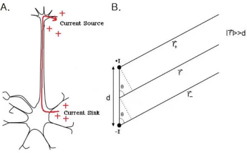
Figure 2: Model of extracellular potential generated by a single action potential. A: Positive ions flow into and out of a neuron due to one action potential. B: Model of the neuron as a current dipole. The length of the neuron from dendrite to
axon terminal is d. There is a current sink at the dendrites and a current source at the axon terminal. The distance from the midpoint of the dipole to the point of measurement is 𝒓⃗ . The point of measurement is so far away that 𝒓⃗ , 𝒓⃗⃗⃗⃗ +, and 𝒓⃗⃗⃗⃗ −
can be assumed to be parallel
When a neuron undergoes an action potential, positive ions flow into the dendrites and cell body of the neuron. The positive ions then travel down the axon and flow out of the axon terminals, see Figure 2A. From the perspective of an extracellular electrode, this flow of ions constitutes a current sink at the dendrites and a current source at the axon terminals. This separation of a current sink and source by a short distance may be modeled as a current dipole. Figure 2B illustrates a model of a single neuron as a current dipole, where the points marked ±I represent the current source and sink, d represents the length of the neuron, and 𝑟⃗⃗ is the distance
from the midpoint of the neuron to the point of measurement. If we make the simplifying assumption that ions flow isotropically towards/away from a current sink/source, the magnitude of the current density becomes
|𝐽 | = |𝐼|
4𝜋𝑟2, (1)
4
confined to travel along prescribed paths, such as wires in electric circuits. Instead, the more general form of Ohm’s Law must be used,
𝐽 = 𝜎𝐸⃗ . (2)
This form applies to situations in which currents may be conducted throughout a three-dimensional volume. 𝜎 is the conductivity of the physical or biological material, and 𝐸⃗ is the electric field. In this case, 𝜎 is the conductivity of the neural tissue in between the neuron and the point of measurement. 𝜎 is assumed to be a scalar for simplicity, though in general it is a tensor. If we assume the current density resulting from a current source or sink is isotropic throughout space, then 𝐸⃗ is also isotropic, pointing away from a current source and toward a current sink. Using equation 2, we can derive the potential V at a distance 𝑟+/− away from a
single current source or sink. Combining equation 1 and equation 2, we obtain
𝐸⃗ = 𝐼
4𝜋𝜎𝑟+/−2 𝑟̂+/− , (3)
where I is positive for a current source and negative for a current sink. Note that equation 3 has the same form as the electric field due to a point charge. The potential therefore takes the same form as that of a point charge:
𝑉(𝑟, 𝑡) = 𝐼(𝑡)
4𝜋𝜎𝑟+/−2 . (4)
Now, using equation 4, we can derive the potential due to a current dipole as
𝑉(𝑟, 𝑡) =|𝐼(𝑡)| 4𝜋𝜎 ( 1 𝑟+− 1 𝑟−) . (5)
where 𝑟+ is the distance from the current source to the point of measurement and 𝑟−is the
distance from the current sink to the point of measurement. Here, we assume that the current source and sink have the same magnitude of current at all points in time because the time scale of an action potential is at least ten times faster than the fastest frequency component of EEG
5
recordings. Assuming r >> d, the three vectors 𝑟 , 𝑟⃗⃗⃗ +, and 𝑟⃗⃗⃗ − can be assumed to be parallel to each other. 𝑟⃗⃗⃗ + and 𝑟⃗⃗⃗ − can be rewritten as 𝑟 ±𝑑
2cos 𝜃. Substituting these into equation 5, we
obtain 𝑉(𝑟, 𝑡) = 1 4𝜋𝜎 |𝐼(𝑡)|𝑑 cos 𝜃 (𝑟2−𝑑2 4 cos2𝜃) . (6)
Since r >> d, equation 6 can be further simplified to
𝑉(𝑟, 𝑡) =|𝐼(𝑡)|𝑑 cos 𝜃
4𝜋𝜎𝑟2 . (7)
Equation 7 computes the potential at distance r and angle θ from a dipole current sink and source. We interpret this to be the theoretical potential at the scalp due to the activity of one neuron [4]. It should be emphasized that this is a highly simplified model where we assumed the extracellular conductivity, σ, to be a scalar, and the direction of 𝐽 , current density, to be
isotropic. Nonetheless, this model still provides useful insight into how EEG rhythms emerge from the activity of millions of neurons [3].
1.3
Frequency Bands
The most conventional way to analyze EEG signals is to observe their spectral content. Even before it was understood how EEG signals were generated, it was recognized that the amplitude and frequency of oscillations in recorded brain activity provide information about a subject’s brain state. EEG frequency ranges are categorized into five different bands based on peak spectral power: delta (below 4Hz), theta (4 to 8 Hz), alpha (9 to 13 Hz), beta (14 to 29 Hz), and gamma (above 30 Hz) [5]. Classically, delta waves are prominent during sleep, theta waves are associated with deep relaxation and dreaming, alpha waves emerge during relaxed
wakefulness with eyes closed, beta waves are associated with attention and concentration, and gamma waves correspond to critical thinking and extreme focus [6]. How these rhythms are
6
generated within different brain regions is still not fully understood [7]. Much work is currently being done to determine the biophysical mechanisms underpinning these various rhythms, especially in clinical contexts [5].
1.4
Apparatus
We decided to utilize a Muse Headband [8], a low-cost commercial EEG headset to record EEG signals. The commercial purpose of the Muse Headband is to pair with a smartphone app and help the user increase the quality of meditation in real-time. While not designed for research purposes, the Muse Headband can nonetheless be used to acquire raw EEG signals that could, in principle, form the basis of a BCI. In this regard, we were able to route the real-time EEG signals from the MUSE headband into Matlab.
More specifically, the Muse Headset uses Open Sound Control (OSC) as its main network protocol. OSC was designed for musical performance and show control, thus it works great for real-time data transmission and receiving. The EEG signals need to be obtained simultaneously to run the cooperative task in real time. The exact same portal as the OSC
network has to be opened in the Matlab program to connect the Muse Headband to the computer and receive the real-time signal. However, this real-time signal is not in the format we desire. Matlab codes designed by the company that created OSC was used to decrypt EEG signal in real time. Next, the real-time EEG signal was fully accessible for signal processing.
1.5
Objectives
The project aims were thus:
1. To design a simple binary classifier which receives individuals’ brain/EEG signals and distinguishes between relaxed and concentrated mental states. The classifier allows a user to
7
engage the BCI when they are concentrating and disengage when they are relaxed. The
classifier is based on techniques from Discrete-time Signal Processing and Machine Learning.
2. After the methods for distinguishing between relaxed and concentrated states are refined, design a cooperative task in Matlab. In this task, two subjects work together to direct a ball to an acceptance range given a prescribed path. We initially proposed a task in which each subject is responsible for the ball’s motion in either the x-axis or the y-axis. This is to say that for our original task, an individual who is responsible for the ball’s horizontal motion cannot influence the ball’s vertical motion whatsoever and vice versa. Towards the end of the project, we adjusted our task so that one subject is responsible for the direction of the ball’s motion and the other subject is responsible for the displacement of the ball’s motion, refer to Figure 3. Together, they form the vector of the ball’s movement. The task has been transformed from the Cartesian coordinates to the polar coordinates.
3. To experimentally verify the design of the cooperative BCI. We gathered multiple subjects to test the designed BCI system on the cooperative ball-moving task.
8
Figure 3: A Diagram of the Cooperative Task. The blue ball is controlled by two subjects who switch from relaxed and focused states of mind. One subject is responsible for the direction of the ball, θ, and the other subject is responsible for the displacement of the ball, r. Each subject take turns to reach the ball to the acceptance range. If the ball were to move
9
Chapter 2
Methods I: Spectral Analysis
2.1
Theories of Discrete Fourier Transform
To observe and determine which EEG frequency band is dominant over a certain duration of time, the Fourier Transform is used to transform a segment of EEG signal from the time domain to the frequency domain. Fast Fourier Transform (FFT), a computationally faster version of the Discrete Fourier Transform (DFT), was used in Matlab to observe the signal in the frequency domain. A standard DFT synthesis equation is shown below:
X(k) = ∑ 𝑥(𝑛)𝑒−𝑗(
2𝜋 𝑁)𝑛𝑘
𝑁−1
𝑛=0 (k = 0,1,2, … , N − 1), (8)
where N is the number of points in x(n), the segment of an EEG signal about to be transformed. The length of DFT will be the same as the number of samples in the segment of the signal. Since all the segments of the signal will be real-valued, the magnitude of Discrete Time Fourier
Transform (DTFT) and the DFT will be symmetric or even [10]. To focus on observing the differences in the DFT of the different segments of the EEG signal, redundant parts were
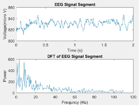
discarded. The power associated with frequencies below the Nyquist frequencies were kept, that is [0,π] in DTFT scale, and all the other values were discarded. Direct Current (DC) terms were ignored by subtracting the mean of the EEG signal segment from each sample in the EEG signal segment [10]. Figure 4 shows a segment of EEG signal and the DFT of the segment with
modifications. With a sampling frequency of 220 Hz, the Nyquist frequency is 110 Hz. Since DFT over 440 samples are taken, the size of the frequency bin is 0.5 Hz. DFT over more samples would allow for smaller frequency bin and better resolution in the DFT. In figure 4, the DC term has been subtracted in the frequency domain, but not in the time domain.
10
Figure 4: A two-second segment of EEG signal obtained from the Muse headband and the DFT of the segment are plotted. Note that the highest frequency bin in the DFT is 110 Hz due to the sampling frequency of the Muse headband
220 Hz.
2.2
Time-frequency Spectrograms
With hundreds of two-second-long data, it would be nearly impossible to observe and compare each two-second-long DFT manually. In practice, a spectrogram is used to observe pattern or changes in the frequency contents of the signal over time. A spectrogram is a three-dimensional plot where the magnitude of DFT is plotted against the frequency and the time [10]. Even with the same dataset, the spectrograms can appear very different depending on the various parameters. These parameters consist of the type of window, the length of window, and the number of samples overlapped. The EEG signal is divided in time over a particular window with certain length. Note that the overlapped sample should always be smaller than the number of samples being transformed. After each transform, the DFT is stacked next to each other to show what power or magnitude at what frequency dominates at what time. For example, in Figure 4,
11
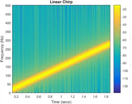
the segment of EEG signal is windowed with a rectangular window transformed using DFT. The specific DFT is one strip of the spectrogram. Figure 5 is an example of a spectrogram of a linearly increasing chirp, where the frequency content of the signal is increasing linearly with respect to time. Note that we can point out at what time, what frequency ranges are dominant and how a dominant frequency range changes over time. These features of the spectrogram are taken into consideration while designing a classification algorithm for the BCI. The spectrogram in Figure 5 is artificially generated and clean, hence it possible to eyeball the features of the spectrograms. However, features of the spectrograms with actual data are difficult to discern with the naked eye.
Figure 5: A spectrogram of a linear chirp is plotted. The frequency content of the signal is increasing linearly with respect to time. Using a spectrogram, hidden patterns could be observed if one were to expect changes in the frequency contents
of a signal.
The type of window is essential in observing and detecting patterns in the signal. The Fourier Transform of any finite length signal or samples is equivalent to the convolution of the Fourier Transform of the signal and the Fourier Transform of a window. If there were no specific
12
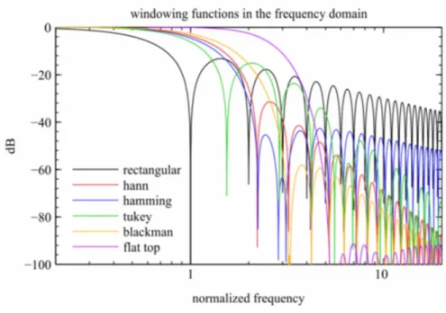
window multiplied to the signal, it is assumed that the signal has been rectangular windowed. Each window has its pros and cons. However, the main trade-offs among different windows arise from the width of the main lobe and the height of the side lobes in the DTFT of the windows (refer to Figure 6). With larger width of the main lobe, the resolution of the
spectrogram decreases. With taller height of the side lobes, the blurring effect increases. Most of the windows tend to have larger width of the main lobe when the height of the side lobes
decreases and vice versa. Thus, there is a trade-off between the resolution and the blurring effect of the spectrograms [10]. Different types of windows are shown in Figure 6. In this project, different windows were investigated and compared for our purpose. Note that the Fourier Transform of the finite-length signal is convolved with these functions. In general, with rectangular windows, there are less contrast between the frequency bins compared to other windows. Thus, in practice, most of the time, rectangular windows are not used.
Figure 6: DTFT of different windows in dB are plotted respect to normalized frequency. Note that the rectangular window has the narrowest main lobe and the highest side lobes. Blackman window, on the other hand, has wide width in
13
Another important parameter in creating a spectrogram is the length of the window. Depending on the length of the window, the number of samples Fourier Transformed is going to differ. With more number of samples, the size of the frequency bins is decreased. This is a way to compensate for some of the windows with large width in the main lobes. With longer window length, the relatively larger resolution can be compensated. However, longer window length means longer wait time and delay in the BCI system. Thus, another trade-off is formed in which we obtain a more accurate spectrogram with a longer window length, but a longer delay between each new input for the BCI system.
14
Chapter 3
Methods II: Feature Extraction and
Classification
3.1
Classification
Patterns were identified from the spectrogram observations for both concentrated and relaxed states. To classify the two states, we used a learning stage and testing stage. The purpose of the learning stage is to provide our algorithm pre-classified labeled data from which the algorithm can use to predict the labels of new data [11]. For this algorithm, Linear Discriminant Analysis (LDA) and Support Vector Machine (SVM) were used for the classification. The advantage of LDA is that the algorithm and the concept is simple while being mathematically robust [12]. LDA is based on the concept of searching for a linear combination of feature variables. With each new viable feature variable, the threshold that classifies two states, should become more accurate. Developed by Fisher in 1936, LDA is defined by the following score function, S(𝛽), S(𝛽) =𝛽 𝑇𝜇 1− 𝛽𝑇𝜇2 𝛽𝑇𝐶𝛽 , (9) Z = 𝛽1𝑥1+ 𝛽2𝑥2 + ⋯ + 𝛽𝑛𝑥𝑛, (10) 𝐶 = 1 𝑛1+ 𝑛2 (𝑛1𝐶1+ 𝑛2𝐶2), (11)
where Z is the classifier. μ1 and μ2 are the mean vectors for the two subsets that we wish to
15
covariance matrices for each subset. 𝑥1 through 𝑥𝑛 are features of the datasets. The linear coefficients, β1, β2,…, βn can be estimated to maximize the score function,
𝛽 = 𝐶−1(𝜇
1− 𝜇2) (12)
Note that for two variables, Z becomes a line, for three variables, a plane, and for four variables, a hyperplane. The calculation has an analytic solution which makes LDA very easy to implement while some other classifiers use optimization, such as support vector machine. There are some simplifying assumptions about the data: the data are Gaussian, which means each feature, when plotted, have a bell curve shape and values of each variable vary around the mean by the same amount in average. With these assumptions, the LDA model estimates the mean and variance of the data and makes predictions by estimating the probability that the new data belongs to a class [11].
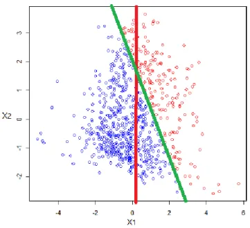
An example of LDA is shown in Figure 7. Since there are two variables, X1 and X2, the LDA threshold, or Z, is a line. If the classification algorithm finds a threshold that is not a linear combination of each variable and finds a threshold with respect to X1, the red line becomes the threshold. The red dots on the left side of the threshold and blue dots on the right side of the threshold would be considered the error or mislabeled datasets. With LDA implemented in the classification algorithm, the green threshold becomes the new threshold where the error is minimized. The solution to Fisher’s equation consists of a threshold that is a linear combination of the variables. If, for any reason, the new feature does not contribute to the classification, the weight on the feature is zero.
16
Figure 7: Two datasets plotted with respect to features or variables, X1 and X2. Observing the X1 feature of the two datasets, the red line would be a linear threshold that classifies the two dataset. However, with one more feature, X2, the
green line becomes the new linear threshold. Note that the error in classification with the green line is much lower than the error with the red line [13].
In the example depicted in Figure 7, the combination of X1 and X2 together is most powerful. In consideration of X2 feature alone, there are too much overlaps to draw a threshold separating the two datasets. Therefore, the choices of features are essential. The LDA algorithm provides a threshold that has the least overlap between two data subsets [11].
Another widely used method to classify two sets of data is Support Vector Machine (SVM). SVM makes no assumption on the data at all and focusing on minimizing the number of misclassified data points using ‘slack variables’ within some range of overlap [14]. This means that SVM does not focus on the entire set of data but a subset where there are overlaps [14]. The points used for the optimization is called support vector because they determine where the discriminator should lie. Solving the following optimization problem gives the linear discriminator of the two datasets.
17
subject to 𝑎𝑇𝑥
𝑖 − 𝑏 ≥ 1 − 𝑢𝑖, 𝑖 = 1, … , 𝑁
𝑎𝑇𝑦𝑖 − 𝑏 ≤ −(1 − 𝑣𝑖), 𝑖 = 1, … , 𝑀
𝑢 ≽ 0, 𝑣 ≽ 0,
Where xi and yi are the datasets, ui is measure of how much 𝑎𝑇𝑥𝑖− 𝑏 ≥ 1 is violated and
similarly for vi, 𝛾 is the relative weight of the number of misclassified point compared to the
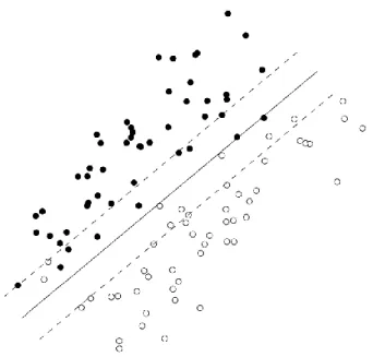
width of the slab. By finding a, b, and nonnegative u and v, we can find the optimal linear classifier using SVM. a is the coefficients or the weights on the features and b is the threshold for the linear combination of the features. An example of SVM is shown Figure 8. Note that 𝛾 is used to maximize the width of the slab while minimizing the number of misclassified points. Unlike LDA, SVM focuses on the slab in between the support vectors to find the optimizing threshold rather than using the whole dataset. We slightly adjusted the thresholds to fit our purpose better in the cooperative task.
Figure 8: Linear discriminator using support vector machine with some value γ is shown with solid line. The linear discriminator classifies three of the points wrong. By using support vector machine, the number of misclassified points
18
3.2
Weber Contrast
As mentioned above, many classical BCIs operate by extractive power in certain frequency bands from EEG signals. Thus, we wanted to characterize the observed peaks at the alpha bands and relatively low activities at theta and beta bands as a feature. Rather than the absolute summed power of the alpha waves, the contrast of the alpha band with respect to theta and beta bands were utilized in the LDA. Weber contrast, shown below, was used to characterize the peak:
C =𝐿𝐹− 𝐿𝐵
𝐿𝐵
, (14)
where 𝐿𝐹 is the luminance of the feature and 𝐿𝐵 is the luminance of the immediate adjacent background [15]. For our purpose, 𝐿𝐹 represents the absolute summed power of the alpha band
activities (9 – 13 Hz) and 𝐿𝐵 represents the absolute summed power or intensity of the theta and
beta bands (4 to 8 Hz and 14 to 29 Hz). We neglected the intensity of the theta bands due to some artifacts in the data. The specific artifacts were observed in the theta bands (<7 Hz) due to eye movements, especially during concentration. The artifacts due to eye movements were minimal during relaxation due to the eyes being closed. We took the contrast of alpha activities with respect to the beta activities as a feature for classification.
3.3
Information Transfer Rate
To quantify the effectiveness of our BCI algorithm, the information transmission rate (ITR) was calculated to be able to compare with similar prior BCI research. To calculate the rate at which information was transmitted per second, we need the concept of mutual information to quantify the degree to which knowledge of a subject's brain state enabled us to accurately decode the intended action. We can interpret the user's intended action as a binary stimulus (stop or
19
move), and the decoded action also as a binary response (which is ideally the same as the intended action). Both can be modeled as random variables (e.g., 0 corresponding to stop, 1 corresponding to move). If knowing the response (i.e., the decoded action) reduces uncertainty about the stimulus (i.e., the user's intended action), then information is shared between these variables, which we can quantify using mutual information [16]. The mutual information of this system is obtained by 𝐼𝑚= − ∑ 𝑃[𝑠] log2𝑃[𝑠] − (− ∑ 𝑃[𝑟]𝑃[𝑠|𝑟] 𝑠,𝑟 log2𝑃[𝑠|𝑟]) 𝑠 (15)
where r and s represent response and stimulus. P[r] and P[s] are the probability distributions associated with these variables. P[s|r] is the probability of s stimulus (e.g., the intended action of stop) presented when r response (e.g., the decoded action to stop) was observed. The first term in Equation 15 represents the uncertainty in the user's intended action, without knowledge of the user's brain state. The second term represents the uncertainty in the user's intended action with knowledge of the user's brain states. High mutual information therefore indicates that the knowledge of brain waves reduces a large uncertainty in the user's intended action. Zero mutual information means that knowledge of subject's brain state does not help to determine the user's intended action. ITR is computed by dividing the mutual information by the total transmission time, which in our case was the length of newly arrived EEG data in time (0.5 seconds). This rate can be used to evaluate how our algorithm compares to other similar BCIs.
20
Chapter 4
Methods III: Data Acquisition and
Experimentation
To acquire data from the Muse Headband as accurately as possible, the following procedures have been implemented.
Procedures Before Acquiring Data:
1. Wipe the electrodes of the headband as cleanly as possible with rubbing alcohol.
2. Check that the subject’s scalp is in good contact with the headband via Muse Headband App.
Procedures for Calibration:
1. For relaxed state, subjects close their eyes and clear their mind.
2. For concentrated state, subjects count backwards silently from multiples of 100s with a decrement of three.
Procedures for Measurement:
Set the portal number while running Muse-io.exe and the portal number indicated in the Matlab program the same. Note that there should be one portal open for each subject. If the cooperative task requires three subjects, there would be three Muse-io.exe and three Matlab programs running at the same instance. Once the data for both states has been acquired, spectrogram from the data will be analyzed in real time to ensure that the subject is able to properly enter both states. High gamma activities and peaks at alpha bands should be observable,
21
else the calibration is repeated. The data acquired from calibration is used to determine the threshold for distinguishing between relaxed and concentrated states.
Both subjects perform the above procedures every time before attempting the collaborative tasks.
Experiment Subjects
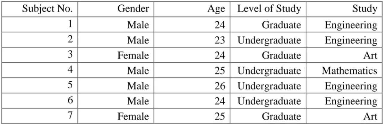
There were total of seven students including myself who participated in this experimental test. The goal of this minimal risk experiment was thoroughly explained to the students. If they expressed interest, the students voluntarily became the subjects without any reward. The sessions and cooperative task trials were held at night after dinner. Sessions were rescheduled if the students had a stressful or busy day. The length of the sessions was 8 ~10 minutes long where there were at least 5 minutes of training session and 3 minutes of testing session. The sampling frequency of the EEG signals were 220 Hz. After the training session, we used the data from the training session to run the classification algorithm. The classification algorithm informed us on the weights of the features and error rates associated with the data from the testing session for both LDA and SVM methods. The subjects gave the permission to give away the following information:
Subject No. Gender Age Level of Study Study
1 Male 24 Graduate Engineering
2 Male 23 Undergraduate Engineering
3 Female 24 Graduate Art
4 Male 25 Undergraduate Mathematics
5 Male 26 Undergraduate Engineering
6 Male 24 Undergraduate Engineering
7 Female 25 Graduate Art
22
Chapter 5
Results
The result consists of three parts: (i) observations and results from the EEG signals of the mental states, (ii) the classification of the EEG signals using LDA and SVM and its performance in terms of the error rate and ITR, and (iii) the verification of the cooperative task.
5.1
Spectrum and Spectrogram
Different lengths of the window and lengths of overlaps were investigated to allow for the signal processing and ensuing cooperative task to be performed in real-time. To try to compensate for a longer delay due to longer window length, the number of overlapped samples between the previous and next DFT was increased. In particular, we considered windows of length 440 samples with an overlap of 330 samples (110 new EEG samples added to each window). Thus, with a sampling frequency of 220 Hz, the length of each window being Fourier Transformed was two seconds long. The BCI system updated each time the 110 new EEG samples were added; new classification of EEG signals twice every second due to a sampling frequency of 220 Hz.
The EEG signals acquired during concentrated and relaxed states were measured and observed, with general EEG phenomology agreeing with the literature [5]. The two-second-long segments of the EEG signals for both states were plotted and shown in Figure 9. While the subject is relaxed, the alpha EEG frequency band is expected to be dominant in the signal. Note there were about 19 large oscillations within 2 second period. Peaks at around 10 Hz was
23
was relaxed, the signal while the subject was focused had much larger high frequency contents. Magnitude of the DFT of these two signals are shown in Figure 9.
Figure 9: Segments of EEG signal while the subject is under relaxed and focused states are plotted. Higher frequency contents are expected while the subject is focused. Lower frequency contents are expected while the sujbect is relaxed. Compared with the spectrum with the relaxed subject, the spectrum while subject is focused has higher powers at frequencies higher than 30 Hz. There is also high power at around 10 Hz in the spectrum while subject is relaxed.
24
More intense gamma activities were observed in the spectrum while the subject is focused as compared to the spectrum of the relaxed subject. Previous findings on gamma activities in the frontal lobe inform that the subject’s state of mind is under concentration, focused attention, or learning [5]. The levels of gamma activities varied every time the headsets were newly put on. We speculated that there exists a subject varing electrode position where the noise of the EEG signals is minimized and that the signal to noise ratio can vary depending on where the electrodes are placed. Thus, it was impractical to record systematic numerical responses for each mental states; The power of each frequency bins varied each time the
headsets were newly worn. As expected from the number of oscillations in the EEG signal while subject is relaxed, there was a peak at around 10 Hz in the spectrum. These two observeations in each electrode were used as the feature variables in the classification algorithm.
In order to visualize how the power spectral density varied with time, we analyzed spectrograms: As before, each spectrogram utilized a Hamming window, with a sliding window length of 440 samples, and the overlap of 330 samples. Figure 10 shows spectrograms while the subject was in a focused state. Figure 11 shows spectrograms while the subject was in a relaxed state. Each figure has two spectrograms, one from the EEG recordings on the right side of the frontal lobe (Electrode 1) and the other from the left side of the frontal lobe (Electrode 2).
Qualitatively, there is minimal difference in the spectrograms across the two different electrodes. There are more activities in the right hemisphere during comparison task and in the left
hemisphere during the multiplication and bilateral during subtraction task [18]. In this regard, it is worth noting that the sources of stimulating concentration were randomly generated
25
quantitavely observed in our data. This was mainly due to the poor contact between the scalp and the electrodes.
Figure 10: Spectrogram of the EEG signals while the subject was focused with Hamming window with window length of 440 samples and overlap of 330 samples. The high gamma power is observed at frequencies above 30 Hz at most time interval. The stripes in the spectrogram and the irregular high powers at low frequencies were artifacts from the data
26
Figure 11: Spectrogram of the EEG signals while the subject was relaxed with Hamming window with window length of 440 samples and overlap of 330 samples. Most of the power at frequencies above 30 Hz at most time interval were realatively low. High power at around alpha frequencies were observed for most time interval. The high power artifacts
at low frequencies were low compared to the the Figure 10.
In the spectrograms while the subject was relaxed, we observed relatively high alpha activities on the frontal lobe. This narrow band-like behavior at around 10 Hz was systematic across all the spectrograms while the subject was relaxed. Much higher gamma activities (> 30 Hz) were observed during concentration. In an effort to characterize delays in switching from one brain state (focused/relaxed) to the other, the subject was told to switch states whenever a beep sound was heard (beep at t = 40, t = 90, t = 120, t = 170, and t = 200). The result of this experiment is depicted in Figure 12.
27
Figure 12: Spectrogram of the EEG signals while the subject was relaxed and focused for different intervals with Hamming window with window length of 440 samples and overlap of 330 samples The intervals colored in grey in the
spectrograms were the intervals while the subject was told to relax. High power at around 10 Hz and low powers at
frequencies higher than 30 Hz were observed in these intervals.
From t = 0 to t = 40, t = 90 to t = 120, and t = 170 to t = 200 seconds, the subject was told to be relaxed. During the time intervals in between when the subject was relaxed, the subject was in a focused state. Bands at around 10 Hz were observed while the subject was relaxed. The gamma activities during focused states were much higher than the gamma activities during relaxed states. The powers from 22 Hz to 110 Hz were summed to observe total beta and gamma activities in the frontal lobe. For this specific dataset, the summed power when the subject was relaxed averaged at around 5000 for both electrodes. The summed power when the subject was concentrating averaged at around 9000.
28
The Weber contrasts were higher for the relaxed state, and lower, negative number for the concentrated state. Referring back to equation 13, the contrast is expected to be high and positive when the subject is relaxed because the power at the alpha band are large. The numerator of equation 13 is large compared to denominator. However, while the subject is concentrating, the power at the alpha bands is low relative to the adjacent frequency bands. The numerator of equation 13 becomes negative (refer to Figure 13).
5.2
Classification and Information Transfer Rate
To classify the received EEG signal into either the relaxed or concentrated state, we used the two features: the gamma activities and the contrast between alpha and beta waves. Each feature for each electrode is plotted in Figure 13. For this specific training set, we observed a large overlap in gamma activities for relaxed and concentrated states. However, even with the poor separation in the summed power of the gamma activities, we observed that LDA on the two features for each electrode classifies the two mental states with a relatively low error rate.
29
Figure 13: Four features are plotted with respect to the number of samples. Note that these numerical values for the features are not one of the best datasets. Rather, these values are in one of the worse cases of an example subject, which could be due to poor contact with the scalp or the subject is unable to focus or relax. The threshold of LDA was defined by the cross of the linear combination of the features for relaxed and concentrated state. Despite the indistinguishable
gamma activities, LDA algorithm on all the features show a low error rate, around 15 percent.
The weights on the feature variables relied more heavily on the contrast at alpha bands than the summed power of gamma activities for both LDA and SVM method, refer to Table 2 and 3. We observed lower weight on the absolute sum of power at gamma frequency bands compared to the weight on the contrast on alpha frequency band. However, this is reasonable since the numerical
30
values of the contrasts were in the magnitude of decimal places while the absolute sum of the power at gamma frequency bands were in the magnitude of hundreds.
Subject No. Weight on Gamma Activities from Electrode 1 Weight on Gamma Activities from Electrode 2 Weight on Alpha Activities Contrast from Electrode 1 Weight on Alpha Activities Contrast from Electrode 2 1 -0.0002 0.0003 -0.0016 -0.0014 2 0.00001 0.0001 -0.0016 -0.0019 3 0.00001 -0.0001 -0.0025 -0.0016 4 -0.00001 -0.00001 -0.0019 -0.0023 5 0.00001 0.00001 -0.002 -0.0022 6 -0.0001 0.0001 -0.004 -0.0025 7 -0.0002 0.00001 -0.0029 -0.0045
Table 2: The weights on each feature for each subject implemented with LDA.
Subject No. Weight on Gamma Activities from Electrode 1 Weight on Gamma Activities from Electrode 2 Weight on Alpha Activities Contrast from Electrode 1 Weight on Alpha Activities Contrast from Electrode 2 1 0.0458 -0.0843 0.8908 1.1781 2 0.0181 -0.0583 0.8966 0.8087 3 -0.0006 0.0255 1.3416 1.6788 4 0.0023 -0.0014 1.2645 1.0754 5 0.0007 0.0017 1.5173 2.1467 6 0.1476 -0.0404 1.2646 1.2633 7 0.094 0.0059 1.6 1.7708
Table 3: The weights on each feature for each subject implemented with SVM.
The error rates and ITR were computed for each subject with the test data, refer to Table 4. The threshold for LDA was determined by the position of the cross between linear
combination of the features for relaxed and concentrated states. The true negative, true positive, false negative, and false positive was computed using the weights and thresholds of the features from LDA and SVM and the testing session data, i.e. probability of subject concentrating when classification of concentration was detected, probability of subject concentrating when
31
classification of relaxation was detected, probability of subject relaxed when classification of concentration was detected, and probability of subject focused when classification of relaxation was detected. These probabilities were used in equation 15 to compute the mutual information. For this binary system, the maximum mutual information is 1 bit. The maximum ITR is 2 bit/s because the transmission time is 0.5 second. Furthermore, we achieve a higher ITR as a BCI system because the BCI requires more than one subject to drive the ball. In Table 4, we observed lower error rate with the classification using SVM than the classification using LDA. Hence, we used SVM weights in the real-time cooperative task. The ITR of a typical visual cortex
stimulating BCI for a single subject is around 1~1.7 bit/s [19].
Subject No. Error Rate with LDA (%)
Error Rate with SVM (%)
Information Transfer Rate (bit/s) 1 13.68 13.46 0.82286 2 15.38 15.17 0.7612 3 16.24 14.74 0.7200 4 8.55 7.26 1.1576 5 6.41 4.70 1.3242 6 25.21 19.02 0.3708 7 24.36 25.00 0.3980
Table 4: Error rates and information transfer rate for each subject. The error rate of the classification implemented with SVM was systematically lower than that of LDA. Note that the error rate varied largely, which directly affects the ITR of
the BCI.
We made some manual adjustments to the threshold. If our hypothesis is that the
concentration influenced the action (the ball’s angular or radial movement), false positive is that the relaxation influenced the action and false negative is that the concentration did not influence the action. By increasing false negative, we can increase the true negative (relaxation did not influence the action). This minimized the ball’s accidental movement (classifying relaxed state) when the subject wanted to hold the ball in place (subject was relaxed).
32
5.3
Cooperative Task
Each subject demonstrated the task with one another for three times, i.e. subject 1
demonstrated with subject 2 for 3 trials, demonstrated with subject 3 for 3 trials, and so on. As a result, each subject completed 18 trials with different subjects as their partner. The starting location of the ball was at (0,0) and the acceptance range were from ([250 275], [250 300]) (Start point circled red and the acceptance range shown in a rectangle in Figure 14). The subjects pair had total of 10 minutes to finish the task. The velocity of the moving ball was set to 1.5 unit per second and the angular velocity of the ball was set to 2𝜋
144 radian per second. The velocity and the
angular velocity was designed such that the task can be completed under 4 minutes. Subject pairs (1, 4), (1, 5), (2, 4), (2, 5), (3, 4), (4, 5) were successful in driving the cursor to the acceptance range. A trajectory of successful cooperative BCI task is plotted in Figure 14. Figure 15 depicts the linear combination of the features and the threshold. If the linear combination of the features was larger than the threshold, the mental state of the subject was classified as concentration. If the We were more likely to observe a successful completion of the task if the ITR of the subject pair was high. We also observed that the time limit was not a problem and that all the failures to drive the ball to the acceptance range was due to driving the ball out of the prescribed path.
33
Figure 14: The trajectory of the cursor driven by subject 4 and 5.
34
Chapter 6
Discussion
6.1
Artifacts and Distortion
Although the cooperative task had been successfully demonstrated by some subject pairs, most subject pairs had hard time driving the ball to the acceptance range. Once the subjects moved the ball to a desired position, the excitement distracted the subjects’ ability to relax. Nonetheless, the ball was successfully controlled by two individuals contributing in different basis vectors that could not be interrupted by one another. One individual had no control over the direction of the ball and the other had no control over the displacement of the ball.
The binary BCI control can be improved by compensating the eye moving artifacts we observed in our EEG signals. Eye moving artifacts could be due to blinks, eyelid flutters, eyeball movements [17]. We observed eye blinks artifacts in our data, which has “U” shape voltage readings, shown in Figure 16. Eyelid movements produces rhythmic 2-6 Hz activities [17]. Note that none of these artifacts were visible in EEG signal or spectrograms while the subject was relaxed since the subjects closed their eyes to stimulate calm, resting mind. In the power spectrum and spectrograms while subject is focused, high power from 1-8 Hz were randomly observed. Thus, we discarded the theta activities in the EEG signals when computing for the contrast at the alpha waves.
35
Figure 16: A segment of the EEG signal while the subject is focused. Fast oscillations are observed, thus high frequency contents can be expected in the DFT. The large “U” shape dip at around 1.5 second is a voltage drop due to an eye blink.
This voltage drop would cause high power at low frequencies in the DFT.
As expected from DSP theories, there were trade-offs between the blurriness and the resolution of the spectrogram for using different windows. By using rectangular window, color difference between each frequency bins were more distinct compared the spectrogram using Blackman window. However, we observed more blurring in the rectangular window. The overall color of the spectrograms was much brighter with rectangular windows than the other windows since the voltage rms of the EEG signal is reduced when windowed with Hamming and
Blackman window. Hamming window was used in this analysis as this window seemed to be the mid-point of the trade-off between the resolution and the blurriness of the spectrogram.
36
Figure 17: Spectrogram was created with different type of windows. First spectrogram was created using rectangular window. The second spectrogram was created using Hamming window. The third spectrogram was created using Blackman window. From using rectangular window and Blackman window, a trade-off between the resolution and the
blurriness of the spectrogram was observed.
Window length of 440 samples were chosen to obtain higher resolution of the spectrogram. With more samples in the DFT with fixed sampling frequency, the size of the frequency bin would decrease. Using Hamming window instead of rectangular window brings the contrast between the frequency bins up because the height of the side lobe of the FT of Hamming window is taller than that of rectangular window. Having more samples or increasing the window length compensates the decrease in the resolution of the spectrogram due to
Hamming windowing. However, longer window length would also mean a delay and temporal blurring in the classification of the two states. With window length of 440 samples and sampling
37
frequency of 220 Hz, there could be at most 2 second delay in the input. However, if the subject is relaxing or concentrating extremely well and depending on how the threshold is set, this two second delay could be reduced.
Unexpected harmonic distortions were visible throughout the project. The same distortions were observed regardless of the activities at different frequencies. These artifacts occurred regardless of how well the headband was in contact with the forehead. The artifact was investigated thoroughly in frequency and time domain in attempt to find a fix. The artifact is shown in Figure 18. From observing one strip of the harmonic distortion, we concluded that the harmonic artifacts look very similar to impulse trains or square waves. Using DSP, we
characterized the shape of the inverse FFT. Since there was an impulse every 2 Hz, we can expect 2 impulses per second in the time domain. The shape of the signal in the time domain should have a resembalance of an impulse train.
38
Figure 18: A stripe of the Artifact seen in the spectrogram. Note there are about 50~60 peaks, which breaks down to 1 peak every 2 Hz. From Inverse FFT, 2 impulses per second is expected in the time domain.
An impulse behavior in time domain was observable in the Figure 19. From t=3 to 5 seconds, There were roughly 2 oscillations or 2 impulses per second which was correctly
predicted from the FFT. Note that there was another artifact from t=11 to 13 seconds which was confirmed in the powerspectrum. As expected, the shape of the signal in the time domain
resembled an impulse train where the peak voltage was the same and that the signal decays down to 0. These behaviors were also visible in the second artifact. Most of the artifacts were around 2 to 3 seconds long.
39
Figure 19: Segment of the time domain signal is shown in the above plot and the Spectrogram using Hamming Window is shown in the below plot. The artifacts are visible in both the time domain signal and the spectrogram from t= 3 to 5
seconds and t= 11 to 13 seconds.
One way to remove the artifact is using a different window. List of some of the windows are shown in Figure 20. As mentioned, there are trade-offs between the blurriness and the resolution of the spectrogram while using different windows. This was easily seen in the above figure, where there were some blurring at 3.5 seconds and 5.5 seconds. With a rectangular window, we observed less blurring effect in the spectrogram. Also, the power at each bin was significantly decreased as the window becomes narrower. This is expected as the signal is losing its information away from the center when it is being windowed.
40
Figure 20: Different windows are shown in the plot. M represents the length of the signal windowed. Note that if the signal is a rectangular wave, the harmonic behavior in the Fourier Transform will be greatest in the rectangular window and
least in the Blackman window. Note also that the power of the Fourier Transform will be reduced due to the window.
With a narrower window, we can effectively reduce the effect of the artifact. However, the blurriness which erases the effect of the artifact can also decrease the gamma or alpha activities. Since our classification algorithm is influenced largely by these factors, we kept our Hamming Window. After many observations of the time domain signal of the artifact, we concluded that these signals are mismeasured from the Muse Headband. The voltage readings seemed to be copied and pasted over to the right. In our task, we kept the last FFT such that if an artifact of this kind emerges, the game will use the last FFT instead of the artifact to decide the mental state. In the codes for real-time task, the last features of the DFT were saved. If there were more than certain number of oscillations in the new DFT which dips below -50 dB, the old features of the DFT were used instead of extracting the new features from the new DFT.
6.2
Signal Processing
In the real-time cooperative task, the linear threshold was modified such that the
41
have more control over holding the ball still. However, this modification forced the subjects to concentrate harder to move the ball’s rotational or radial movement. In Figure 21, the test data and the linear threshold are plotted respect to time. Note that we can clearly observe when the subject is relaxed or focused.
Figure 21: Transformation of the four features is plotted respect to time in blue. LDA threshold is shown in red.
The EEG signals varied largely in magnitudes and frequencies among different datasets. One of the biggest problems was the contact between the electrodes and the scalp. Every time, the subject took off the headband, it was highly unlikely that the headband would be placed on the same position. Thus, every time the headband was newly placed, the subject was required to run a session of practice tests. A training session, written in Matlab, outputted the new weights for each feature and the threshold. During the session, the subject was randomly told to switch
42
between states for about 5 minutes. After the training session, there was a test session, where the subjects relaxed and focused, to compute the error rate and the ITR.
There were differences in the numerical values of the features depending on the subject’s condition. The subjects had relatively higher gamma activities throughout the day compared to the night. The contrast at alpha bands were higher during the night than the day. Some subjects felt that the sitting posture on the chair was not comfortable, which caused problem relaxing. Many factors were not able to be closely controlled due to subtle differences between
individuals.
There were a few limitations to the Muse headband. Unlike any other EEG equipment, the advantage of Muse headband was that it was very simple to wear and to start gathering EEG signal. However, due to no conducting medium, such as jell or saline, the voltage readings by the Muse headset were quite noisy. We believed that the harmonic distortions were due to bad conducting medium and that the voltage recording had been copied over to make up for the lost data. Because there was no conducting medium, it was essential that all the electrodes were in contact with the skin very tightly. If there were too much grease on the skin or on the electrode, the EEG signals sometimes had higher mean voltage. Because we were unsure if the signal was better with grease on the skin, we wiped the electrodes and foreheads with rubbing alcohol every time for systematic purposes. The sampling frequency of the Muse headband was 220 Hz. The highest frequency component that spectrum could have was 110Hz. If the sampling frequency was higher than 220 Hz, we could use the information from the magnitudes at frequencies higher than 110 Hz to characterize noise. By characterizing the noise, the spectrogram could be filtered for better feature extraction.
43
One way to improve the classification of two mental state is to discard the outliers of the data set. Outliers of the set change the mean and the variance of the data, which has impacts on LDA method. One way of achieving this task is by elliptical peeling [14]. Elliptical peeling allows us to peel the furthest point away from the clumped data point one by one. After the furthest point has been discarded, a new discriminator is solved. If we are unhappy with our result, we can peel of the next furthest point until there are no points left, which then we know that the outlier of the dataset had no large impact on the discriminator.
44
Chapter 7
Conclusions
We designed a cooperative BCI task in Matlab where the two subjects work together to direct a ball to the acceptance range. Switching from different mental states, the subjects had the control to engage and disengage the BCI at will. Although not all the subject pairs were
successful in driving the ball to the acceptance range, we observed the feasibility of cooperative BCI task.
Through investigating spectrograms and optimizing the window types and length, different patterns were observed and studied. Most low frequency components, below 8 Hz, were mainly due to eye movements that cause artifacts in the spectrograms. Eye blinks caused large dips in the voltage readings and eyelid movements caused 2~8 Hz oscillations in the EEG signal. Gamma activities, above 30 Hz, were dominant while the subjects were focused. Peaks at 10 Hz were observed in the spectrograms while the subjects were relaxed. Studies and literatures on EEG signals inform that alpha activities, 8 to 13 Hz, are dominant during patient’s relaxed, calm state [5].
Linear Discriminant Analysis (LDA) and Support Vector Machine (SVM) were
incorporated in the classification algorithm and compared. In the training session, the algorithm received the pre-classified data and outputted the weight on each feature and the threshold for classifying relaxed and focused state. We used the summation of the gamma activity and the contrast at alpha band as the features of the dataset.
We observed systematically less error rate in the test data with SVM method than with LDA method. In the real-time cooperative BCI task, we used the weights and thresholds from
45
SVM algorithm. We computed ITR, which is one of the measures of the effectiveness of a BCI. The average ITR of this BCI was 0.8 bit/s. The ITR of a typical visual cortex stimulating BCI is at 1~1.7 bit/s [19].
46
Chapter 8
References
[1] Jonathan Wolpaw and Elizabeth Winter Wolpaw, Brain- Computer Interfaces: Principles and Practice, Oxford Scholarship Online, May 2012.
[2] Farwell, L., and Donchin, E. (1988). Talking off the top of your head: toward a mental prosthesis utilizing event-related brain potentials. Electroencephalogr. Clin. Neurophysiol. 70, 510–523.
[3] Poli, R., Cinel, C., Matran-Fernandez, A., Sepulveda, F., & Stoica, A. (2013, March). Towards cooperative brain-computer interfaces for space navigation. In Proceedings of the 2013 international conference on Intelligent user interfaces (pp. 149-160). ACM.
[4] Rall, W. and Shepherd, G.M. Theoretical reconstruction of field potentials and
dendrodendritic synaptic interactions in olfactory bulb. J. Neurophysiol. 31: 884-915, 1968. [5] Niedermeyer, E. and Lopes da Silva, F. (editors) Electroencephalography (4th edition), Williams and Wilkins, Baltimore, 1998.
[6] Paul L. Nunez, Electric and Magnetic Fields Produced by the Brain In. Brain Computer Interfaces: Principles and Practice, Oxford Scholarship Online, May 2012.
[7] Silva, F. H. Lopes da. “Neural mechanisms underlying brain waves: from neural membranes to networks.” Electroencephalography and clinical neurophysiology 79 2 (1991): 81-93. [8] “Muse | Meditation Made Easy.” Muse: the Brain Sensing Headband,
www.choosemuse.com/.
[9] Paul L. Nunez and Ramesh Srinivasan Electroencephalogram. Scholarpedia, 2(2):1348., revision #91218, 2007.
[10] Discrete-Time Signal Processing (3rd Edition) (Prentice-Hall Signal Processing Series) by Alan V. Oppenheim, Ronald W. Schafer.
[11] B. Suleiman and T. A.-H. Fateh, “FEATURES EXTRACTION TECHNIQUES OF EEG SIGNAL FOR BCI APPLICATIONS.”
[12] Turlapaty, “Introduction to Linear Discriminants,” YouTube, 01-Oct-2013. [Online]. Available: https://www.youtube.com/watch?v=twn5gnyu7ss. [Accessed: 02-Oct-2017].
47
[13] “9.2.10 - R Scripts,” STAT897D - Applied Data Mining and Statistical Learning. [Online]. Available: https://onlinecourses.science.psu.edu/stat857/node/135. [Accessed: 02-Oct-2017].
[14] Boyd, S., & Vandenberghe, L. (2004). Convex Optimization. Cambridge: Cambridge University Press. doi:10.1017/CBO9780511804441
[15] Campbell, F. W., & Robson, J. G. (1968). Application of fourier analysis to the visibility of gratings. The Journal of Physiology, 197(3), 551–566.
[16] Cover, T. M., Thomas, J. A. (2006). Elements of Information Theory 2nd Edition (Wiley Series in Telecommunications and Signal Processing). Wiley-Interscience. ISBN: 0471241954
[17] R. J. Croft, R. J. Barray, "Removal of ocular artifact from the EEG: a review", Neurophysiol. Clin., vol. 30, 2000, pp. 5-19.
[18] Chochon F, Cohen L, van de Moortele PF, Dehaene S (1999) Differential contributions of the left and right inferior parietal lobules to number processing. J Cogn Neurosci 11:617– 630. CrossRef Medline
[19] Nicolas-Alonso, Luis Fernando, and Jaime Gomez-Gil. “Brain Computer Interfaces, a
48
Vita
Jongwoon Kim
736 Eastgate Ave. Apt. #2N, St. Louis, MO 63130 Cell: 314-449-3409
Email: [email protected]
EDUCATION
Ohio Wesleyan University, Delaware, OH
Bachelor of Arts August 2011 - May 2015
Major in Physics
Washington University, St. Louis, MO
Bachelor of Science August 2015 - May 2018
Major in Electrical Engineering and Systems Engineering
Master of Science August 2015 - May 2018
Major in Electrical Engineering
RESEARCH EXPERIENCE
Ohio Wesleyan University, Department of Physics
Student Researcher August 2014 - April 2015
Title: Development of a Simple Brain-Controlled Video Game Advisor: Dr. Christian Fink
• Wrote codes and drivers to connect EEG with computer and access real-time data in Matlab. • Examined the frequency domain characteristics of the brain signals at the optical cortex when flashed with different frequency lights using FFT (Confirm Steady State Visually Evoked Potential).
• Defined threshold for the system with the consideration of information theory (optimize the thresholds such that the information transferred per second is maximized; information was maximized at 0.25 bits per second).
• Built a two degree of freedom game in real-time, where the user controlled a virtual ball to desired location within a time window.
Washington University, Department of Electrical and Systems Engineering
Summer Researcher June 2017 - August 2017
June 2016 - August 2016
Master Thesis September 2016 - April 2018