Deep Learning for Image Spam Detection

San Jose State University

SJSU ScholarWorks

Master's Projects Master's Theses and Graduate Research

Spring 5-20-2019

Deep Learning for Image Spam Detection

Tazmina Sharmin

San Jose State University

Follow this and additional works at:https://scholarworks.sjsu.edu/etd_projects

Part of theArtificial Intelligence and Robotics Commons, and theInformation Security Commons

This Master's Project is brought to you for free and open access by the Master's Theses and Graduate Research at SJSU ScholarWorks. It has been accepted for inclusion in Master's Projects by an authorized administrator of SJSU ScholarWorks. For more information, please contact [email protected].

Recommended Citation

Sharmin, Tazmina, "Deep Learning for Image Spam Detection" (2019).Master's Projects. 702. DOI: https://doi.org/10.31979/etd.b8me-rqsv

Deep Learning for Image Spam Detection

A Project Presented to

The Faculty of the Department of Computer Science San José State University

In Partial Fulfillment

of the Requirements for the Degree Master of Science

by

Tazmina Sharmin May 2019

© 2019 Tazmina Sharmin ALL RIGHTS RESERVED

The Designated Project Committee Approves the Project Titled Deep Learning for Image Spam Detection

by

Tazmina Sharmin

APPROVED FOR THE DEPARTMENT OF COMPUTER SCIENCE SAN JOSÉ STATE UNIVERSITY

May 2019

Dr. Mark Stamp Department of Computer Science

Dr. Katerina Potika Department of Computer Science

ABSTRACT

Deep Learning for Image Spam Detection by Tazmina Sharmin

Spam can be defined as unsolicited bulk email. In an effort to evade text-based spam filters, spammers can embed their spam text in an image, which is referred to as image spam. In this research, we consider the problem of image spam detection, based on image analysis. We apply various machine learning and deep learning techniques to real-world image spam datasets, and to a challenge image spam-like dataset. We obtain results comparable to previous work for the real-world datasets, while our deep learning approach yields the best results to date for the challenge dataset.

ACKNOWLEDGMENTS

I would like to express my sincere gratitude to my advisor, Dr. Mark Stamp, for his extraordinary support, patience, and continuous guidance throughout my project and graduate studies as well.

I would like to thank my committe members, Dr. Katerina Potika and Fabio Di Troia for being very helpful and their valuable time.

My parents, Md. Gofranul Hoque and Ferdousi Rezwan, are my constant source of inspiration. I am extremely grateful for their endless support and love throughout all these years. I would like to thank my husband, Jane Alam Jan, for his gracious support and constant encouragement which made it possible. Last, but not the least, I am thankful to my daughter, Ahona, for her understanding and caring in her little own way during the past few years.

TABLE OF CONTENTS CHAPTER 1 Introduction . . . 1 2 Background . . . 3 2.1 Types of Spam . . . 3 2.2 Image Spam . . . 4

2.2.1 Types of Image Spam . . . 4

2.2.2 Image Spam Filtering Techniques . . . 5

2.2.3 Related Work . . . 6

3 Machine Learning Techniques. . . 8

3.1 SVM . . . 8

3.1.1 Overview . . . 8

3.1.2 SVM Algorithm . . . 9

3.2 Neural Networks . . . 10

3.2.1 Multilayer Perceptron . . . 10

3.2.2 Convolutional Neural Network . . . 11

4 Experiments . . . 14 4.1 Evaluation Metric . . . 14 4.2 Environment Setup . . . 15 4.3 Dataset . . . 15 4.3.1 Dataset 1 . . . 15 4.3.2 Dataset 2 . . . 16

4.3.3 Dataset 3 . . . 16 4.4 Feature Generation . . . 16 4.5 Results . . . 17 4.5.1 SVM Experiments . . . 17 4.5.2 MLP Experiments . . . 20 4.5.3 CNN Experiments . . . 23

4.5.4 Cold Start Experiments . . . 24

4.5.5 Comparative Analysis . . . 27

5 Conclusion . . . 31

LIST OF TABLES

1 SVM Dataset 1 (32×32) . . . 18

2 SVM Dataset 1 (16×16) . . . 18

3 SVM Dataset 2 . . . 18

4 SVM Dataset 3 . . . 19

5 SVM (Combined Features - Raw and Canny)) . . . 19

6 MLP Accuracy . . . 23

LIST OF FIGURES

1 Topology of Multilayer Perceptron . . . 11

2 Schematic Representation of CNN Architecture . . . 12

3 ROC Curve with Shaded Area . . . 15

4 Feature Generation (Raw, Canny and Combination of Raw and Canny) . . . 17

5 ROC Curves for Combined Features . . . 20

6 Proposed MLP Architecture . . . 21

7 MLP Results . . . 22

8 CNN Architecture . . . 24

9 CNN Results . . . 25

10 Cold Start Results - SVM . . . 26

11 Cold Start Results - MLP . . . 26

12 Cold Start Results - CNN . . . 27

13 Comparison of Learning Techniques . . . 28

14 Comparison to Previous Work (Dataset 1) . . . 29

15 Comparison to Previous Work (Challege Dataset 1) . . . 29

CHAPTER 1 Introduction

Electronic mail or email is the most popular communication medium between people across the world [1]. As of 2015, the number of email users was 2.6 billion, while in 2019 this number will rise to approximately 2.9 billion, with more than one-third of world population using email to exchanging messages [2].

However, the effectiveness of email service is often reduced by spam. Spam is unwanted email with a commercial, fraudulent or malicious purpose. As email usage has increased, the number of spam messages has also increased. Text-based filters have been developed to deal with the spam problem. In an effort to evade such filters, spammers sometimes use image spam, that is, spammers can encode their messages as images [3].

Previous research into image spam detection has shown that some types of image spam can be detected with high accuracy. For example, in [4, 5] a wide variety of image properties are extracted and images are classified as spam or ham (i.e., legitimate email) based on machine learning techniques. However, some challenging types of image are difficult to detect using such techniques.

In this research, we carefully conduct experiments to determine the effectiveness of various machine learning algorithms for image spam detection, as a function of the amount of training data available. We analyze a variety machine learning algorithms---including deep learning techniques---over several image spam datasets. These experiments serve two purpose. First, we can determine an effective strategy in the ‘‘cold start’’ case, that is, in the case where the training data is severely limited. And second, we compare the effectiveness of deep learning to other machine learning algorithms for the specific problem of image spam detection.

relevant background topics on image spam and related work in spam detection. Chapter 3 provides an overview of the machine learning and deep learning algorithms considered in this research. Chapter 4 presents our implementation details and experimental results. Finally, Chapter 5 concludes the paper, and we discuss possible avenues for future work.

CHAPTER 2 Background

Spamming means sending unsolicited messages to a large number of users in an arbitrary manner. Initially, the idea of spam originated with the purpose of advertising products. Later, spammers used spam for online deception and fraudulent activities. Since sending spam messages via email add no operational cost, email spam has been found to be economically viable. Hence, spammers have particularly focused on spam email.

2.1 Types of Spam

Types of spam can vary depending on its targeted medium of communication. Various types of spam include email spam, mobile phone messaging spam, web search engine spam and social networking spam [6].

Email spam is unsolicited electronic messages in bulk amount and it is the most widely used spam. In email spam, same messages are sent to numerous email addresses. Those messages may include product advertisements, links to phishing websites which might ask the recipient to provide confidential information or malware installers that look innocent. At the beginning, most email spam contained only text messages. Later, image-based spam email emerged to obfuscate text-based spam filters. Image spam include spammer's message in the form of an image. There is another form of email spam called blank spam [5] that has no message inside the email. Blank spam is used in order to collect legitimate email addresses.

Mobile phone message spam or SMS spam refers to junk message sent to mobile phones which is similar to text messaging through short message service. It causes inconvenience to the mobile phone users and also cost the incoming message [5]. As there are costs associated with SMS spam, it is less common than email spam.

after a query. When a website is detected as having search engine spam, that site is marked and penalized. One survey shows that 51.3% website hacks were related to search engine spam manipulating search engine optimization [7].

Social spam aims at social networking websites like Facebook and Twitter. In social spamming, one primary key factor is creating fake account in social application to hack into valid user account. These fake accounts are used to send bulk messages with similar content or sending malicious links with the intent to harm. As social networking sites became popular over time, social spamming activities like clickbaiting or likejacking have become more common [8].

Gaming spam means sending messages in bulk to players using a common chat rooms or public discussion areas. Spammers target users who like gaming to sell gaming items for real world money or in-game currency.

2.2 Image Spam

Image spam is a subclass of email spam, which has emerged as an obfuscation method to avoid text-based spam filters. It is assumed that most of the image spam are used to advertise products, deceive users to gain personal data or deliver malicious software [6]. It is more challenging to detect image spam as they involve various image creation techniques and randomization algorithms. Several obfuscation techniques are used to create image spam which include, but are not limited to making the text outlines blurry, using multiple image layers to construct an image, adding noise to the image randomly and using animations inside the image.

2.2.1 Types of Image Spam

Image spam have evolved over time and take several forms to bypass the conven-tional anti-spam techniques: text-only image, gray image, sliced image and randomized image.

Text only image is the first generation image spam. It contains pure text embedded into an image. These images look like regular text email which is actually an image. A technique using optical character recognition (OCR) has been employed to extract the texts from images and pass it to the spam filters.

Gray image is difficult to detect as it is often mistaken for a ham image. Gray images often look quite identical to natural gray scale images. So, it is crucial to determine if a gray image is genuine or spam.

Sliced image consists of multiple images merged together in jigsaw puzzle manner. This type of spam image is challenging to detect because the combined images often appear to be genuine and hence get through spam filters.

Randomized image refers to randomization of the image pixels. To make a randomized image, spammers make changes to the individual pixel in the image. As a result, it becomes hard to distinguish the randomized image from the original image. The changes made usually do not affect the appearance of the images to the users but significantly influence the output of OCR technique.

2.2.2 Image Spam Filtering Techniques

There are three categories of techniques used to detect spam images: header based, content based and non-content based techniques.

• Header based techniques: An email header consists of data about the sender and the receiver, i.e., sender IP, sender email address, date, from, to, etc. Header fields of an email contain valuable information which may be useful in distinguishing spam and non-spam email. A portion of email header attributes can be used to train and test machine learning models to provide prediction results [9].

email for particular keywords which are usually found in the body section of spam email. Typically, the body of an email carries the actual information to be delivered. Then the filters use pattern recognition or text classification to determine the specific pattern. One early stage content based filter used OCR for extracting words from the text part of the image and pass them to text-based filters [10].

• Non-content based techniques: Non-content based techniques rely on various image features like color properties and metadata features. It is based on the idea that an image which has been simulated must have some distinguishing properties than a genuine image.

2.2.3 Related Work

Since the evolution of image spam, there have been ongoing research on its detection. Machine learning algorithms play a useful role in this research area. Moreover, several deep learning techniques are being deployed to provide robust detection results.

Gao et al. [3] propose an image spam detection scheme by using probabilistic boosting tree algorithm to predict if a given image is spam or not. They execute feature engineering on color and gradient orientation histogram features to generate feature vectors for learning. In order to generate the training set, they use k-means clustering approach rather than randomly selecting spam images. Once the training set is generated, a probabilistic boosting tree algorithm is deployed on it to classify spam and ham images. For test purpose, 5-fold cross validation is performed. Their experiments obtain an accuracy of 89.44% and 0.86% of false positive rate.

Kumaresan et al. [11] propose their research for detecting image spam based on color features by using k-Nearest Neighbor (𝑘-NN) algorithm. They consider the

histogram properties of an image including RGB color histogram, HSV histogram and combination of these two histograms. The classification of images is done based on this feature set. Their proposed method using k-NN algorithm gives 94.5% accuracy with the combined histograms of RGB and HSV.

In research by Annadatha et al. [5], support vector machines (SVM) has been implemented over 21 image features. Each feature has a weight associated based on how much it has contributed to the classification. They classify images by compiling feature extraction over a selected subset of features. This feature selection method reduces the computational effort. The experiment achieves very high accuracy rate of 97% with area under the curve (AUC) value of 1. From their research, it is observed that SVM is a reasonable approach for image spam detection which actively learns various image properties and achieves a higher accuracy with a low false positive rate.

Chavda et al. [4] conduct two sets of experiments with SVM and image processing. In the first part, they extract 41 image features and achieve 97% and 98% accuracy with two publicly available datasets, respectively. Moreover, they construct two new challenge datasets based on those public datasets using image processing techniques on spam images. In the second part of experiments, they evaluate two feature selection algorithms, namely, recursive feature elimination (RFE) and univariate feature selection (UFS).

Aiwan et al. [12] propose an image spam filtering method based on convolutional neural network (CNN). To detect image spam in real time, they train convolutional neural network using enlarged data samples. The proposed system using data aug-mentation achieves an accuracy improvement by 6% than other methods of data augmentation. Combining CNN and proposed data augmentation method enables spam filtering model to obtain 7% to 11% higher accuracy than that of the traditional method.

CHAPTER 3

Machine Learning Techniques

In this chapter, we discuss the background information on Machine Learning and Deep Learning techniques for image spam classification. In machine learning part, we present an overview of SVM. In the deep learning section, we discuss feed forward neural network and convolutional neural network.

3.1 SVM

Support vector machine (SVM) is a supervised machine learning technique which has been extensively used for in detecting email spam [13] and image spam [14]. In this section, a short overview of SVM is given.

3.1.1 Overview

There are four key ideas of SVM algorithm [15], which is a useful technique for binary classification problems:

• Separating hyperplane: In the training phase, SVM tries to find a decision surface which defines a decision boundary between objects belonging to different classes. In multidimensional space, it attempts to figure out the separating hyperplane that classifies the data into their respective groups. In an ideal case, all data belonging to one class remains in one side of the hyperplane and the other group falls on the other side.

• Maximize the margin: For binary classification, we try to find out an optimal hyperplane. For binary classification, two sets of data are divided with maximum margin of separation between each class and the hyperplane. The margin is defined to the minimum distance between the hyperplane and the closest data point in the training set. Optimal hyperplane is the particular one for which the margin is maximized.

assumed to be a linear function. But there are cases where data points are not linearly separable. Hence, SVM transforms the input space data to a higher dimensional feature space. Although this transformation is expensive, it makes the classification easier by spreading out input data.

• Kernel trick: Kernel trick means a function which transforms data into another dimension. It is used to transform input space to a higher dimensional feature space. The kernel trick does not perform the actual transformations, yet it enables us to find a complex non-linear boundary which is capable of dividing different classes of data. Hence, it is computationally cheaper and very useful in solving complex problem.

3.1.2 SVM Algorithm

Like other machine learning techniques, SVM works in two phases: training phase and testing phase. At the training phase, we build a model which learns from a labeled dataset. At the testing phase, we analyze the prediction results of the generated model as its response to new data. These two phases can be summarized below:

3.1.2.1 Training Phase

For a set of training data, where 𝑋1, 𝑋2, . . . , 𝑋𝑛 are data points and𝑧1, 𝑧2, . . . , 𝑧𝑛

are corresponding set of classification where 𝑧𝑖 ∈ {−1,1}, training a SVM model

consists of two phases:

1. Transforming data points (input space) to high dimensional feature space which is essentially done by the kernel trick.

2. Solving an optimization problem Maximize: 𝐿(𝜆) = 𝑛 ∑︁ 𝑖=1 𝜆𝑖− 1 2 𝑛 ∑︁ 𝑖=1 𝑛 ∑︁ 𝑗=1 𝜆𝑖𝜆𝑗𝑧𝑖𝑧𝑗𝐾(𝑋𝑖, 𝑋𝑗), Subject to: 𝑛 ∑︁ 𝑖=1

This is called solving Lagrangian Duality [15]. The purpose is to find out an optimal separating hyperplane which will clearly divide the feature space into two sets.

3.1.2.2 Testing Phase

In this phase, the model is evaluated based on its accuracy for the test dataset. The datapoint is classified by observing on which side of the hyperplane it remains.

3.2 Neural Networks

Neural networks is a framework for many machine learning algorithms which process composite data inputs through supervised learning. A neural network consists of a collection of nodes and these nodes model the neurons to perform activation for transforming input data to output. Neural networks are used in image classification and there have been many ongoing researches on image classification using deep learning [16].

3.2.1 Multilayer Perceptron

Feed forward neural network using back propagation is an artificial neural network used in classification and regression. It was the first and simplest artificial neural network designed. Feed forward neural network with back propagation is used for classification of image spam using the most optimal feature vectors extracted from an image. It is a supervised learning algorithm to train the neural networks.

Multi layer perceptron (MLP) is the type of neural network consisting of multiple layers with computational nodes, usually interconnected in a feed forward fashion. Each neuron at every layer has a directed interconnection with the nodes in the following layer. Multi Layer neural networks use various learning techniques and back propagation is the most popular one. A MLP has three layers at minimum: an input layer, a hidden layer and an output layer. Other than the input nodes, each node is a

Figure 1: Topology of Multilayer Perceptron used activation function which can be formulated as 𝑆(𝑥) = ₁₊1_𝑒−𝑥 =

𝑒𝑥

𝑒𝑥₊₁.

In back propagation, the output scores are compared with the correct answer to calculate the value of an error function and this error value is then fed backwards throughout the layers of the network. With the help of this information, the algorithm tries to adjust the weight at each connection to reduce the error value. After repetition of this process for several iterations, the whole model converges to the state with a very small value of error function or the change in error value is insignificant. Figure 1 shows a topology of MLP.

3.2.2 Convolutional Neural Network

Generally, neural networks use fully connected layers, that is, all neurons at one layer are connected to all neurons in the next layer. A fully connected layer can deal effectively with correlations between any points within the training vectorsâĂŤregard-less of whether those points are close together, far apart, or somewhere in between. In contrast, CNNs are designed to deal with local structureâĂŤa convolutional layer cannot be expected to perform well when crucial information is not local. The benefit of a CNN is that convolutional layers can be trained much more efficiently than fully connected layers.

For images, most of the important structure (edges and gradients, for example) is local. Hence, CNNs would seem to be an ideal tool for image analysis and, in fact,

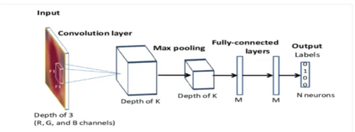
Figure 2: Schematic Representation of CNN Architecture

CNNs were developed for precisely this problem. How- ever, CNNs have performed well in a variety of other problem domains. In general, any problem for which there exists a data representation where local structure predominates is a candidate for a CNN. In addition to images, local structure is key in the fields of text analysis and speech analysis, among many others.

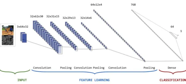
A CNN consists of an input layer, multiple hidden layers and an output layer. Each layer has the common property that it transforms an input to an output with the help of some function that may or may not have parameters. The hidden layers consist of convolution layer followed by pooling layer and then again convolution and pooling layers consecutively, depending on the size of the network. Convolutional layer is a primary building block of CNN which does most of the heavy computational tasks. It implements a convolution operation on the input and the result is passed to the next layer. This layer essentially computes the output values of the neurons which are connected to the local regions of inputs. The computation involves a dot product between the weights of the neurons and a small region in the input volume they are connected to. Figure 2 shows a symbolic representation of CNN architecture.

Pooling layer tries to reduce the number of parameters and amount of computation in the network. It essentially attempts to control overfitting through the reduction of spatial size of the network. There are two types of pooling operations, average pooling

and max pooling. Max pooling is commonly used in CNN applications. It performs a downsampling operation by extracting the maximum parameter and dropping the rest. The last layer is a fully connected layer where the neurons are fully connected to all the activations from previous layers.

CHAPTER 4 Experiments

This chapter presents the empirical analysis and results of our experiments. We discuss about the datasets used and criteria for evaluation followed by experiments and results.

4.1 Evaluation Metric

We evaluate the proposed technique based on accuracy. Accuracy measures how accurately the model has classified a spam as spam and a ham as ham. True positive (TP) is the number of correctly identified samples. False positive (FP) represents the number of incorrectly identified samples. True negatives (TN) are number of negative examples labeled as negatives and false negatives (FN) are number of positive examples labeled as negative. Accuracy can be represented in terms of TP, FP, TN and FN as

Accuracy= TP+TN

TP+TN+FP+FN

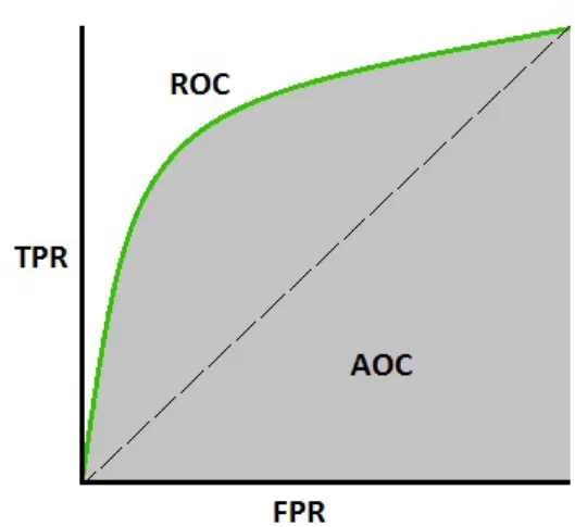
In machine learning, performance evaluation is a crucial task. When a classifica-tion problem is considered, we can count on the AUC of an ROC curve to quantify the performance of the classification problem. A receiver operating characteristic (ROC) curve is a probability curve which is used to compute the area under the curve (AUC) value. By analogy, Higher the AUC value, better the model at classifying between spam and ham images. ROC curve is graphically plotted with true positive rate (TPR) against false positive rate (FPR) at various threshold setting. Figure 3 shows ROC curve with shaded area. The area of the shaded section is computed to determine the AUC value. This value generally lies in between 0.5 to 1. Having an AUC value of 1 is an ideal situation with no false positive or negative.

Figure 3: ROC Curve with Shaded Area

4.2 Environment Setup

All of the experiments have been deployed on a Macbook machine with 8 GB RAM. We use Python for generating the learning models, OpenCV for image processing tasks, Scikit-learn library to implement machine learning algorithms [17], Numpy for mathematical functions and Tensorflow libraries for deep learning training and testing.

4.3 Dataset

Not many image datasets are available to the public due to privacy issues. We use one public dataset which contains actual spam and ham emails exchanged in real time. Moreover, we conduct our experiments on two other datasets generated to challenge existing detection technique.

4.3.1 Dataset 1

The dataset was developed by authors of Image Spam Hunter [3] from North-western University. The dataset contains 920 spam images and 810 ham images. All of the images have jpg/jpeg format.

4.3.2 Dataset 2

This dataset was created by Chavda et al. [4] using image processing techniques on spam images to make them appear more like a ham image. A public corpus named Spam Archieve [18] consists of only spam images. They use this corpus and use a weighted overlay technique to blend those spam images on the ham images from dataset 1.

4.3.3 Dataset 3

This dataset was also developed by Chavda et al. [4] by using a different overlay technique.For this dataset, the background of spam images was deleted and the resulting image was then overlaid onto a ham image. This makes the spam text easier to read, as compared to dataset 2, and according to the results in [4], also makes for a somewhat more challenging detection problem.

4.4 Feature Generation

We consider byte data to construct our feature vector. In the datasets, we observe that the images are of different size. Hence, to maintain consistency, we resize all of the images into 32×32 dimension. To build the feature matrix, we generate byte

data for each pixel in an image. Each pixel is contained in three bytes and each byte represents red, green and blue (RGB) color information within the range from 0 to 255. For computational convenience, each number is mapped into the range of 0 to 1 for the resized matrix. Thus, the feature matrix consists of byte information features for each raw and canny image where each feature vector has 3072 components.

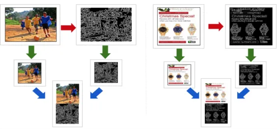
In the next phase, we transform each raw image into a canny image by following canny edge detection technique. Later, we merge each raw and the corresponding canny image to form a new image. This new image has a dimension of64×32and each

Figure 4: Feature Generation (Raw, Canny and Combination of Raw and Canny) features. We use raw, canny and the combination of these two feature vectors to train our models. Figure 4 shows a visual representation of the feature generation process we propose and use in our project. On the left side of the diagram, we transform a raw ham image into a canny hame image, followed by resizing these two images into the same dimension and lastly making the combined feature vector. The right side of the diagram depicts the same procedure that we follow for a spam image.

4.5 Results

We conduct our experiments with SVM, feed forward neural network and convo-lutional neural network. This section contains experimental details and results.

4.5.1 SVM Experiments

For our experiments, we generate separate SVM models for each of the three datasets. In each dataset, we perform a random shuffle and use 70% of the image samples for training and the remaining 30% for testing. In all of these SVM experiments we test both linear and RBF kernels.

Table 1 shows the accuracy of the SVM when trained and tested on Dataset 1, using the raw images resized to 32 ÃŮ 32. When using the RBF kernel, we achieve

an accuracy of 0.9748, which is better than the 0.9156 accuracy with the linear kernel. For comparison, we also build another SVM based on the Canny images. In this case, the accuracy drops to 0.9156 and 0.8492 for the RBF and linear kernels, respectively. We observe that for the SVM, the results for the raw images exceed those for the Canny image. 4.5.1.1 Dataset 1 Table 1: SVM Dataset 1 (32×32) 32×32 Raw Canny RBF 0.9748 0.901 Linear 0.9156 0.8492

Next, we give results for an analogous set of experiments, but with the images resized to 16 ÃŮ 16, giving us feature vectors of length 768. Here, we do sightly better than the 32 ÃŮ 32 case when using the rbf kernel, but worse for the linear kernel.

Table 2: SVM Dataset 1 (16×16)

16×16 Raw Canny

RBF 0.9752 0.9048

Linear 0.8838 0.7861

4.5.1.2 Dataset 2 and Dataset 3

Table 3: SVM Dataset 2

Dataset Raw Canny

RBF 0.7885 0.5553

We conduct our experiments on datasets 2 and 3 using both raw and canny images. Table 3 shows the results for dataset 2. From the results we observe that for both raw and canny image features, we achieve higher accuracies with rbf kernel while with linear kernel the accuracies are below 0.50. As these challenge datasets were specifically designed to make classification using an SVM model more challenging, these results are not unexpected. Table 4 shows the accuracies obtained for dataset 3.

Table 4: SVM Dataset 3

Dataset Raw Canny

RBF 0.6715 0.6271

Linear 0.6433 0.5965

4.5.1.3 Combination of Raw and Canny Features

Table 5: SVM (Combined Features - Raw and Canny))

Dataset RBF Linear

Dataset 1 0.9872 0.9806 Dataset 2 0.7265 0.6939 Dataset 3 0.6896 0.7183

Since we have tested each dataset on raw and canny image features individually, in the next phase, we build another SVM model on combined raw and canny image byte features. Table 5 presents the results from our experiments on the three datasets. We tune the model with rbf and linear kernel. Our experiment achieves slightly better accuracy for dataset 1 with rbf kernel. For dataset 2, our model yields an accuracy of 0.7265 with rbf kernel which is better than 0.6939 obtained from using linear kernel. On the contrary, for dataset 3, our SVM model performs well when we tune it with linear kernel, yielding an accuracy of 0.7183 against 0.6896 with rbf kernel. From the

(a) Dataset 1 (RBF) (b) Dataset 2 (RBF) (c) Dataset 3 (Linear)

Figure 5: ROC Curves for Combined Features

results, it is observed that for dataset 1, SVM technique performs well on combined features than using raw or canny features individually. But, for dataset 2, it is not the same case where we can see that our proposed SVM approach provides better results with raw image features alone . For dataset 3, combined features yield higher accuracy results in comparison with the accuracies from training with individual features.

Figure 5 gives the ROC curves for the best SVM result for each dataset, based on the combined (raw and Canny) features. As given in Table 4, the corresponding AUC values are 0.9872 for Dataset 1, 0.7265 for Dataset 2, and 0.7183 for Dataset 3.

4.5.2 MLP Experiments

To experiment with Multilayer perceptron (MLP) for classifying spam and ham images, we explore several architectures. The results reported here are for an MLP

with one input layer, two hidden layers and one output layer. For each 64×32

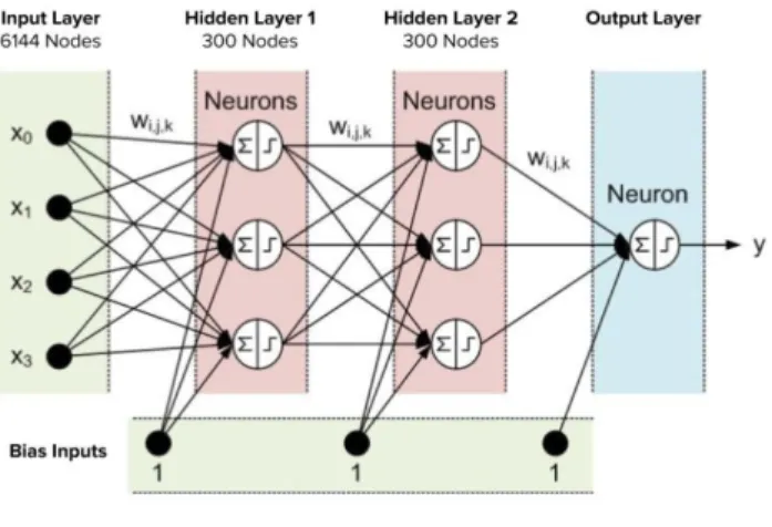
image, the input layer consists of 6144 nodes. Moreover, each hidden layer has 300 nodes and uses rectifier linear unit (ReLU) as activation function. To measure the loss, we selected binary cross entropy loss function. A sigmoid score function is used at the output stage. Our MLPs are trained on 70% of the image samples, and the models are trained for 100 epochs. At each epoch, a batch size of 64 is used, and the validation split is taken as 15% of the image data samples. We activate early stop

Figure 6: Proposed MLP Architecture

as regularization technique to prevent the proposed MLP from overfitting. Figure 6 shows the architecture of the MLP we use in this research.

We achieve an accuracy of 0.96 after testing the MLP on the remaining 30% images. Figure 7a shows MLP model accuracy over 100 epochs. The loss graph in Figure 7b shows that the model is converging with no overfitting.

Next, we conduct similar experiments using the MLP over datasets 2 and 3. The analogous MLP accuracy and loss curves are given in Figures 7c and 7d. Once the iteration stops, we observe that there is a big difference between the training and test accuracies. Moreover, there is no apparent overfitting or underfitting in the loss graph because the difference between training and test loss becomes very small after the first few epochs.

Figure 7e presents training and validation accuracy over dataset 3. The model iterates through 21 epochs. It is visible that when the model stops training, the test accuracy is less than the training accuracy. Figure 7f shows model loss where the model converges with no overfitting or underfitting .

sum-(a) Accuracy Dataset 1 (b) Loss Dataset 1

(c) Accuracy Dataset 2 _{(d) Loss Dataset 2}

(e) Accuracy Dataset 3 _{(f) Loss Dataset 3}

Figure 7: MLP Results

marized in above. In comparison to the SVM results, we see that the MLP fails to outperform the SVM on any of the three datasets. Also, on Dataset 2, the MLP is very poor, performing no better than a coin flip.

Table 6: MLP Accuracy Dataset Accuracy Dataset 1 0.9557 Dataset 2 0.5885 Dataset 3 0.6605 4.5.3 CNN Experiments

Convolutional neural networks provide some advantages—both in terms of effi-ciency and accuracy—for image analysis. As with the SVM and MLP experiments discussed above, we apply CNNs to each of the three datasets under consideration.

We experimented with various CNN hyperparameters, but for all of the experi-ments reported here, we use the following configuration. We use three convolution layers following the input layer. The first two con- volution layer has 32 filters. Layer two has 64 filters. Each layer has a kernel size of 3×3. We downsample the data

via a max pooling layer, using a 2×2 pool size. From the last pooling layer, 768

input features are derived and flattened, which are fed to a hidden layer containing 64 nodes. We use ReLU activation function to acitivate a subset of inputs from previous layer. Finally the hidden layer is fully connected to the output layer consisting of one node. At this layer, we use sigmoid activation function and cross entropy loss function. Finally an accuracy value is computed as output. Furthermore, in our experiments, to avoid overfitting, we use a dropout rate of 0.5. The batch size is set to 64 for each epoch, and we have a total of 100 epochs. As with our MLP experiments, we use 70% of the data for training and 30% for testing. Figure 8 represents the CNN artchitecture we propose in this research.

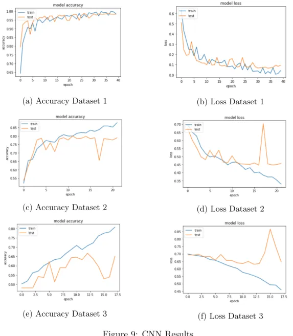
The accuracy and loss graphs for Dataset 1 are given in Figures 9a and 9b, and clearly show that overfitting does not occur. The analogous graphs for Dataset 2

Figure 8: CNN Architecture

appear in Figures 9c and 9d, while the results for Dataset 3 can be found in Figures 9e and 9f. From dataset 2 accuracy graph, we observe that the model iterates through 21 epochs and finally when the model converges we obtain an accuracy of 0.8313. Besides, loss graph exhibits no overfitting or underfitting in the model. Accuracy graph for dataset 3 shows that once the model converges there is a significant difference between training and test accuracies. Corresponding loss graph suggests that the model is overfitting the data in this dataset as the difference between validation land training loss is notable.

The optimal CNN testing accuracies for the three datasets under consideration are given in Table 7. From these results, we see that our CNN outperforms both the SVM and MLP on Datasets 1 and 2 , and does nearly as well as the SVM on Dataset 3.

4.5.4 Cold Start Experiments

Next, we evaluate the three models, namely, SVM, MLP and CNN, in the âĂIJcold startâĂİ case, that is, the case where the training data is limited. We

(a) Accuracy Dataset 1 (b) Loss Dataset 1

(c) Accuracy Dataset 2 _{(d) Loss Dataset 2}

(e) Accuracy Dataset 3 _{(f) Loss Dataset 3}

Figure 9: CNN Results Table 7: CNN Results Dataset Accuracy Dataset 1 0.9902 Dataset 2 0.8313 Dataset 3 0.6769

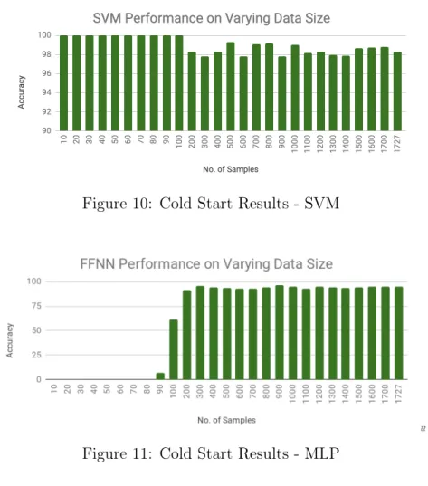
Figure 10: Cold Start Results - SVM

Figure 11: Cold Start Results - MLP

start our experiment with just 10 samples for training, and we gradually increase the number of samples used to train the models. Every result reported in this section is based on 10 separate experiments, with the training data randomly selected for each experiment. For a specific number of samples, we plot the maximum accuracy from the 10 iterations.

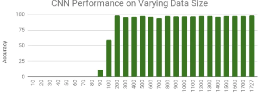
We generate each chart by plotting the number of samples in x-axis and accuracy in the y-axis. The chart in Figure 10 shows the accuracies from experiments with SVM. Figures 11 and 12 give the accuracies of our cold start experiments for MLP and CNN models, respectively.

Figure 12: Cold Start Results - CNN

case as we see for the first few set of samples, accuracies are very high. Once we train the SVM model with 200 samples or more, accuracy drops down a little and it is approximately around 0.98 for the rest of the sequence of experiments. On the contrary, MLP and CNN models seemingly do not learn adequate enough when number of training samples are as limited as 100 samples or less. Once the models are trained with 200 samples or more, accuracy rises above 0.90 and the graph stays smooth through the rest of the experiments.

4.5.5 Comparative Analysis

In this section, we analyze the comparative results of the proposed techniques. From the SVM-based experiments, we observe that we achieve a good accuracy of 0.9872 while for challenge datasets (dataset 2 and dataset 3) it yields 0.7885 and 0.7183, respectively. As these two datasets were generated to challenge existing detection methods, it is intuitive that the proposed technique would not yield as high accuracy as the results obtained for dataset 1. In the next set of experiments, we explore MLP for the three datasets considered in our project. Our proposed MLP approach provides 0.9557 accuracy for dataset 1 while for the two challenge datasets, the learning rate does not improve and we achieve 0.5885 and 0.6605 accuracies, respectively.

Figure 13: Comparison of Learning Techniques

In the following experiments, we implement CNN algorithm to detect spam images. For dataset 1, CNN gives the best accuracy score of 0.9902 among the three proposed techniques. When we train CNN model with images from challenge dataset 1, from the results, it is quite evident that the model learns competently and gives 0.8313 accuracy which is better than SVM and MLP results. On the other hand, CNN experiment for challenge dataset 2 does not yield an accuracy as better as SVM model and we obtain an accuracy of 0.6769. Figure 13 shows the comparative analysis of the accuracies we achieve from our proposed machine learning techniques.

4.5.5.1 Comparison to Previous Work

We conduct another comparative analysis of the results from this research work and previous research in image spam detection. For dataset 1, research by Chavda et al. [4] and Annadatha et al. [5] are considered. We refer to the work in this paper as Research 1, and the work in [4] and [5] as Research 2 and Research 3. From Figure 14, we see that for dataset 1, the highest accuracy previously achieved was 0.97, while our research obtains a better accuracy of 0.9902.

Research 2 generate challenge datasets (dataset 2 and dataset 3) to weaken current detection schemes. For challenge dataset 1, their proposed technique achieves best

Figure 14: Comparison to Previous Work (Dataset 1)

Figure 15: Comparison to Previous Work (Challege Dataset 1)

presents this analysis. For challenge dataset 2, in this research, proposed SVM technique with combined features performs slightly better than the approach in Research 2, with an accuracy of 0.7183 where the highest accuracy they achieved was about 0.70. Figure 16 shows this analysis.

CHAPTER 5 Conclusion

Since the evolution of electronic communication, spam has always been a chal-lenging problem to the cyber world. Hence, it requires substantial attention and a robust detection mechanism. There have been innumerable experimentations of different techniques to detect image spams. Several machine learning techniques have been proven to be quite useful in image spam classification.

In this research, we have analyzed three novel approaches for image spam filtering. One approach includes experimenting with Support Vector Machines and the other two methodologies employ deep learning techniques which are feed forward neural network and convolutional neural network. SVM model is generated by extracting normalized byte blocks of images. The neural network models do not require manual feature extraction. So, we build deep learning models by splitting image data into 70% for training and the remaining 30% for test purpose. We evaluate the model accuracy by tuning several parameters and in multiple iterations. Moreover, we also plot model loss to observe overfitting by taking training and validation data into account. We successfully deploy our models for binary classification of image spams with supervised learning.

Extensive assessment of experiments of various methods on three datasets demon-strates the effectiveness of the proposed approaches. From the results, we observe that CNN-based model achieves higher accuracy on the public dataset and one of the challenge datasets used in the project. As CNN employs convolutions to extract relevant properties at lower computational cost through automatic feature learning, it has been proved to be the most efficacious method in image spam classification.

Future works may include, but not limited to exploring more features related to edges which may guide to new and improved direction in the SVM part. In

addition, further research can be executed by exploring other deep learning techniques such as RNN and LSTM. Moreover, additional tuning of hyper parameters and the architecture may yield more insights in the deep learning network models. Besides, our proposed system can be extended to other image classification problems such as identifying people by recognizing facial expressions or detecting objects (pedestrians, stop signs, etc.) in images. Deep learning Neural networks are capable of uncovering the latent structure from unlabelled data. Hence, training neural networks on image datasets with no label might be another interesting experimentation.

LIST OF REFERENCES

[1] ‘‘How email works,’’ https://runbox.com/email-school/how-email-works/, ac-cessed on March 20, 2019.

[2] ‘‘Email statistics report, 2015-2019,’’ https://www.radicati.com/wp/wp-content/ uploads/2015/02/Email-Statistics-Report-2015-2019-Executive-Summary.pdf, accessed on October 10, 2018.

[3] Y. Gao, M. Yang, X. Zhao, B. Pardo, Y. Wu, T. Pappas, and A. Choudhary,

‘‘Image spam hunter,’’ in 2008 IEEE International Conference on Acoustics,

Speech and Signal Processing, ICASSP, 9 2008, pp. 1765--1768.

[4] A. Chavda, K. Potika, F. D. Troia, and M. Stamp, ‘‘Support vector machines for image spam analysis,’’ in Proceedings of the 15th International Joint Con-ference on e-Business and Telecommunications - Volume 2: BASS,, INSTICC.

SciTePress, 2018, pp. 431--441.

[5] A. Annadatha and M. Stamp, ‘‘Image spam analysis and detection,’’J. Computer Virology and Hacking Techniques, vol. 14, no. 1, pp. 39--52, 2018. [Online].

Available: https://doi.org/10.1007/s11416-016-0287-x

[6] S. Dhanaraj and V. Karthikeyani, ‘‘A study on e-mail image spam filtering tech-niques,’’ in 2013 International Conference on Pattern Recognition, Informatics and Mobile Engineering, Feb 2013, pp. 49--55.

[7] ‘‘Report: 51% of web site hacks related to seo spam,’’ https://searchengineland. com/report-51-of-web-site-hacks-related-to-seo-spam-313468, accessed on March 7, 2019.

[8] ‘‘5 types of social spam,’’ https://thenextweb.com/future-of-communications/ 2015/04/06/5-types-of-social-spam-and-how-to-prevent-them/, accessed on March 9, 2019.

[9] M. Hassan, W. Mirza, and M. Hussain, ‘‘Header based spam filtering using machine learning approach,’’ October 2017.

[10] ‘‘Apache spamassassin,’’ https://spamassassin.apache.org/, accessed on February 13, 2019.

[11] T. Kumaresan, S. Sanjushree, and C. Palanisamy, ‘‘Image spam detection

using color features and k-nearest neighbor classification,’’ International

Engineering, vol. 8, no. 10, pp. 1904 -- 1907, 2014. [Online]. Available:

http://waset.org/publications/10000193

[12] F. Aiwan and Y. Zhaofeng, ‘‘Image spam filtering using convolutional neural networks,’’ Personal Ubiquitous Comput., vol. 22, no. 5-6, pp. 1029--1037, Oct.

2018. [Online]. Available: https://doi.org/10.1007/s00779-018-1168-8

[13] T. Yu and W. Hsu, ‘‘E-mail spam filtering using support vector machines with selection of kernel function parameters,’’ in2009 Fourth International Conference on Innovative Computing, Information and Control (ICICIC), Dec 2009, pp.

764--767.

[14] T. Kumaresan, S.sanjushree, K.suhasini, and C.palanisamy, ‘‘Article: Image spam filtering using support vector machine and particle swarm optimization,’’ IJCA Proceedings on National Conference on Information Processing and Remote Computing, vol. NCIPRC 2015, no. 1, pp. 17--21, April 2015, full text available.

[15] M. Stamp, Introduction to Machine Learning with Applications in Information Security, 1st ed. Chapman & Hall/CRC, 2017.

[16] M. Soranamageswari and C. Meena, ‘‘Statistical feature extraction for classification of image spam using artificial neural networks,’’ in Proceedings of the 2010 Second International Conference on Machine Learning and Computing,

ser. ICMLC ’10. Washington, DC, USA: IEEE Computer Society, 2010, pp. 101--105. [Online]. Available: https://doi.org/10.1109/ICMLC.2010.72

[17] F. Pedregosa, G. Varoquaux, A. Gramfort, V. Michel, B. Thirion, O. Grisel, M. Blondel, P. Prettenhofer, R. Weiss, V. Dubourg, J. Vanderplas, A. Passos, D. Cournapeau, M. Brucher, M. Perrot, and E. Duchesnay, ‘‘Scikit-learn: Machine learning in python,’’J. Mach. Learn. Res., vol. 12, pp. 2825--2830, Nov.

2011. [Online]. Available: http://dl.acm.org/citation.cfm?id=1953048.2078195 [18] M. Dredze, R. Gevaryahu, and A. Elias-Bachrach, ‘‘Learning fast

classifiers for image spam.’’ January 2007. [Online]. Available: https: