Estimation of AUC for Assessing Its Significance in Classification
Models
Okeh Uchechukwu Marius1 Mbegbu Julian Ibezimako2
1. Department of Mathematics and Computer Science, Ebonyi State University Abakaliki, Nigeria. 2. Department of Statistics, Nnamdi Azikiwe University Awka, Nigeria
ABSTRACT
The assessment of the performance of a diagnostic test when test results are measured on continuous scale can be evaluated using the measures of sensitivity and specificity over the range of possible cut-off points for the predictor variable. This is achieved by the use of a receiver operating characteristic (ROC) curve which is a graph of sensitivity against 1-specificity across all possible decision cut-offs values from a diagnostic test result. This curve evaluates the diagnostic ability of tests to discriminate the true state of subjects especially in classification models. These tasks of assessing the predictive accuracy of classification models is always better achieved using a summary measure of accuracy across all possible ranges of cut-off values called the area under the receiver operating characteristic curve (AUC). In this paper, we propose a simple nonparametric method of calculating AUC from predicted probability of positive response involving multiple prediction rules. This method is based on the knowledge of non-parametric Mann-Whitney U statistic. Based on the predicted outcomes and observed outcomes, the performance of diagnostic tests is assessed for the classification models through the AUC calculated from these outcomes. The proposed method when applied on real data, the significance of AUC for the classification models is assessed. The method offers reliable statistical inferences and circumvents the difficulties of deriving the statistical moments of complex summary statistics seen in the parametric method. The proposed method as a non-parametric estimation is recommended for calculating the AUC as it compares favorably with the existing parametric and non-parametric methods.
Keywords: Cut-off value, ROC, Predicted probability, parametric, non-parametric
DOI: 10.7176/JNSR/9-9-03
Publication date:May 31st 2019
INTRODUCTION
In medical sciences, the use of diagnostic procedures is based on clinical investigations or laboratory experiments or trials purposely to classify subject into diseased or non-diseased. These procedures makes for vital decision making aided with advanced machines/tools to detect any given condition. For decades now, receiver operating characteristic curve (ROC) analysis has been used as a popular technique of evaluating the performance or ability of a test to discriminate between alternative health status. The ROC curve represents a graph of sensitivity against 1-specificity across various cut-off values of diagnostic test. It assesses the effectiveness of continuous diagnostic test results to differentiate between groups of healthy and diseased individuals (Greiner et al., 2000; Zhou et al., 2002; Pepe, 2004). It is also a common tool for assessing the performance of various classification tools such as biological test results, diagnostic tests, and statistical distributional models and in assessing accuracy quantitatively or to compare accuracy between tests or predictive models. The ROC curve was originated in the theory of signal detection in the years 1950-1960 (Green and Swets, 1966; Egan, 1975) to discriminate between signal and noise. It has been used in so many areas such as radiology (Metz,1989), psychiatry(Hsiao et al,1989), epidemiology(Aoki et al, 1997), biomedical informatics(Lasko et al,2005). It can provide a direct and visual comparison of two or more diagnostic tests on a single set of scales. It is possible to compare different tests at all decision cut-offs by constructing the ROC curves. For statistical analysis, a recommended numerical index of accuracy associated with an ROC curve are often better used to summarize the information provided for the ROC curve into a single global value or index(Swets and Picket,1982). This index is called area under the ROC curve. AUC takes values between 0.5 (which corresponds to the diagonal ROC curve that passes through the points (0,0) and (1,1)) and 1 (representing perfect test where all cases are correctly classified). AUC represents the diagnostic accuracy of the test Y, so that the larger the area the better the diagnostic accuracy of Y. This means that values closer to 1 indicate that Y optimally discriminates between healthy and diseased subjects, while values near 0.5 indicate that the test is not informative (Zhou et al, 2002). According to Mann-Whitney (1947), AUC is the probability that the observed test result of a randomly selected subject from the diseased population (
Y
1) is larger than the observed test resultof a randomly selected subject from the non-diseased population (
Y
0).For comparing two diagnostic processes,the difference between AUCs is often used. In diagnostic imaging it is generally known that the changes due to subjects represent a major component of the overall changes of the AUC. To better control for the sources of changes when comparing diagnostic tests, a paired study design is often advised because it usually induces positive
correlation between the tests results of the same subjects.
This paper is devoted to reviewing some existing methods of calculating AUC. It attempts to calculate AUC based on a simple new method and evaluate its significance in assessing classification models.
EXISTING METHODS OF CALCULATING AUC
There are several methods of calculating the AUC. All these methods differ in the way the distribution functions of both populations are estimated based on their sample values. In Lopez-Raton et al (2012a), a review of all these methods to estimate ROC curve and AUCs is performed. The two basic methods of estimating AUC are the parametric (bi-normal) and non-parametric (empirical).
Parametric (Binormal ROC curve) method
This estimation is based on the assumption that the test results in the diseased and non-diseased populations or some unknown monotonic transformation of the test results follows a bi-normal distribution. Dorfman and Alf, Jr (1968, 1969) and McClish (1989) proposed maximum-likelihood estimates (MLEs) for the parameters of a bi-normal ROC curve and provided parametric methods for estimating and comparing the partial AUC respectively.
According to Dorfman and Alf (1968), McClish (1989), Metz (1978), suppose that continuous diagnostic test results are normally distributed in the healthy and diseased populations, to be able to properly define ROC curve, let Y denote a random variable representing a continuous diagnostic test result. The diagnosis according to any cutoff value c is positive (diseased) if Y ≥ c and negative (non-diseased) if Y < c. Let D0 and D1 denote the
non-diseased and non-diseased populations, respectively. The true and false positive rates at the cut-off value c, true positive rate, TPR(c), and false positive rate, FPR(c) are
1 0(
)
1 . 1 1
(
)
T P R
c
P
Y
c D
F P R
c
P
Y
c D
Let 2 2 1(
1,
1) ,
0(
0,
0)
1 .1 2
Y
N
Y
N
Where 2 2 1 1 0 0(
,
)
and
(
,
)
are the population mean and variance of the disease and non-diseased group. For any cut-off value c, we have
1 1 0 0
( )
(
)
1 .1 3
( )
(
)
c
T P R c
P Y
c
c
F P R c
P Y
c
where
denotes the standard normal cumulative distribution function. Note also that t is the all possible FPRs according to the varying c values in (−∞, ∞). Simplifying, we have0 0 1 0 0 1 0 0
( )
( )
c
t
c
t
t
c
1 0 0( ).
1.14
c
t
Equation 1.14 is the corresponding cut-off value. Hence
The ROC curve is obtained by substituting for c in equation 1.13 to have the function
1 1 0 0 1 1 1 1
( )
c
( ) .
1.15
RO C t
t
If according to McClish(1989) and Metz(1978), we define
1 0 0 1 0 1 1
,
a
and a
1
1 0
( )
( )
1.16
R O C t
a
a
t
In other to show that AUC measure has an analytic form, we recall and show that
AUC
P Y
(
1
Y
0)
under thebinormal or bi-lognormal ROC curve,
Let
Y and Y
0 1 be two random vectors that are independently drawn from the healthy and diseased population and 0Y
follows lognormal distribution with mean,
0 and variance, 2 0
and
Y
1 follows lognormal distribution withmean,
1 and variance, 2 1
.We here use log transformation to the random vectors
Y and Y
0 1.
SinceY and Y
0 1follows log-normal distribution, then logarithm of
Y and Y
0 1 follows normal distribution. Let1 1 0 0
InY
y and InY
y
be for diseased and non-diseased group respectively, since it is easier to work with normal distribution than the lognormal distribution,
Then
AUC
P Y
1
Y
0
P InY
1
InY
0
P y
1
y
0
This follows that
2 2 1 0 1 0
,
1 0y
y
N
implying that
0 1 1 0 2 2 1 00
P y
y
P Z
1 0 2 2 1 01 . 1 7
A U C
Where
1,
and
0are the means and 2 2 1,
0
are the variances of the result
y and y
1 0 respectively.This is the form AUC takes if binormality is assumed. The AUC can be obtained numerically by substituting the estimated values of the parameters given as
2 2 1 0 1 0
垐
,
,
垐
,
from the sample data.
Alternative method of calculating AUC.
Based on the bi-normal assumption, we know that
0 0 1 1 1 0 1 0
(0,1)
y
(0,1)
y
Z
N
and Z
N
1 0 1 0 1 0 1 1 1 0 0 0 1 1 0 0 0 1 1 1 0 0 0 1 2 2 2 2 0 1 0 1 0 1 0 1 0 1 1 0 2 2 2 2 2 2 2 0 1 0 1 0 1 0(
)
(
)
(
) 0
(
) 0
1
1
1
AUC
P Y
Y
P InY
InY
P y
y
P Z
Z
Z
Z
P Z
Z
P
P Z
P Z
1 0 2 2 2 1 0 1
Therefore 1 0 1 1 0 2 2 2 0 1 0(
)
1.18
1
a
AUC
P Y
Y
a
where
(.)
is the cumulative standard normal distribution function (Pepe,2003;Metz,1986;Zou et al,1997;Hanley and McNeil,1982).Estimating Variance of AUC
2
2
2 1 1 0 0 1 0 0 1 0 0 1 0 1垐
2
2
ˆ
垐
(
)
; (
)
1.19
2
2
n
a
n a
n
n
a
V a
V a
n n
n n
where
n and n
1 0 are the numbers of diseased and non-diseased study subjects, respectively. The variance ofAUC
)
can be estimated by substituting estimators for the parametersa and a
1 0.
To estimate the variance ofAUC, recall that
1 0 2 2 1 01 . 2 0
A U C
The maximum likelihood estimate of δ is obtained substituting the MLE’s of the means and variances.
The MLE of AUC is found by substituting the MLE’s of the means and variances into equation 1.20 and using numerical integration. The AUC now reduce to
1 2 0ˆ
ˆ
ˆ
1 .2 1
ˆ
1
a
A U C
a
Since
ˆ
is a monotonic increasing function of
ˆ
, it is enough to find the variance and standard error of
ˆ.
Since
is a function of the parameters,2 2
1
,
0,
1and
0
,we will adopt the Delta method (Zhou et al, 2002) for finding the approximate variance and standard error for
ˆ.
By definition,
2 2 2 2 2 2 1 0 2 1 2 0 1 0 1 0 2 2 1 0 2 2 1 0 1 0 1 0 2 2 2 0 1 2 2 2 2 0 1 0 1 0ˆ
垐
垐
( )
(
)
(
)
(
)
(
)
垐
垐
2
2
,
1
1
V
V
V
V
V
Cov
Cov
n
2 2 4 2 4 1 0 0 1 0 1 3 3 2 2 2 2 1 2 0 2 1 1 0 1 0ˆ
ˆ
(
)
2
(
)
2
1
1
2
n
n
n
Hence the variance expression for
ˆ
can be obtained using the following expression
2 2 4 2 4 0 1 0 0 1 1 3 2 2 2 2 1 0 1 0 1 0 1 0(
)
1
ˆ
( )
1.22
(
1)
(
1)
垐
2
V
n
n
n
n
The variance of
AUC
ˆ
or
ˆ
can be obtained by substituting the estimated values of2 2
1
,
0,
1and
0
in the above expression. The standard error
ˆ
( )
SE
of
ˆ
is just the square root of the above expression for the variance of estimated AUC. To determine the asymptotic 100(1-α) % confidence interval for AUC, we have
2
垐
. (
)
(
)
1 .2 3
C I A U C
Z
V
Where
is the level of significance and 2Z
is the critical value of Z for a two tailed test at level of significance
.
2
NON-PARAMETRIC (EMPIRICAL ROC CURVE) METHOD OF CALCULATING AUC
Some methods using the empirical ROC curve are the trapezoidal rule to approximate AUC by integration, the Mann-Whitney statistic and the empirical method by DeLong et al. (1988).
Nonparametric (conventional) Delong et al method
The empirical (nonparametric) method by DeLong et al. (1988) is a popular and best known method to compare two correlated AUCs by using the theory of generalized U statistics. They used the structural components method provided by Sen (1960) to generate consistent variance estimates of the elements of the variance-covariance matrix of a vector of U statistics, and the resulting test statistic has asymptotically a
2
distribution. This method isimportant as it helps to study the behavior of the type I error and the statistical power of the conventional nonparametric test for comparing two AUCs over a wide range of relevant parameters and against various alternatives. According to Delong et al. (1988), let the variance of
Y
1 being the component of the ith subject fromthe diseased population,
V Y
(
1i)
be defined as
0 1 1 0 1 01
(
)
,
1 . 2 4
n i i j jV
Y
Y
Y
n
and the variance of
Y
0 being the component of the jth subject from the healthy population,V Y
(
0j)
be defined as
1 0 1 0 1 11
(
)
,
1 . 2 5
n j i j iV Y
Y
Y
n
where
n and n
1 0 are the number of diseased and non-diseased subjects respectively. WhileY and Y
i1 j0are the diagnostic test result of the ith subject with disease and the diagnostic test result of the
jth
subject without disease respectively and
is a function comparingY and Y
i1 j0 such that
1 0
11 00 1 01
,
,
0.5
,
0
,
i j i j i j i jif Y
Y
Y Y
if Y
Y
if Y
Y
The empirical AUC is estimated as
0 1 1 1 0 0 1 1
(
)
(
)
1 .2 6
n n E m p ir ic a l i j i jA U C
V Y
n
V Y
n
The variance of the estimated AUC is estimated as
1 0 2 2 1 0
1
1
(
E m p ir ic a l)
Y Y1 .2 7
V A U C
S
S
n
n
Where 1 0 2 2 Y YS and S
, the variances of the diseased and non-diseased subjects is defined as
2 2 1 1
1
(
)
,
0,1.
1
i i n Y i i Empirical iS
V Y
AUC
i
n
The variance of 0 2 YS
is similarly defined.THE TRAPEZOIDAL RULE AND MANN-WHITNEY U STATISTIC METHODS
To calculate the AUC using the Trapezoidal rule, first the ROC curve is separated into many segments, the area of each segment is computed by joining the points (sensitivity, Se, 1-specificity, Sp) at each interval value of the continuous test results and draws a straight line joining the x-axis. This forms several trapezoids and the AUC can be easily calculated directly by summing the area of the trapezoids that are formed below the connected points making up the ROC curve.
According to Bamber(1975), Hanley and McNeil (1982), the area under an empirical ROC curve, when calculated by the trapezoidal rule, is equal to the Mann-Whitney two sample statistics applied to the two samples since the nonparametric analog to the t-test is the Wilcoxon rank-sum test, or synonymously the Mann-Whitney U test. Here, the possible diagnostic test results for each cutoff value c are considered, and the corresponding true
and false positive rates are calculated by 1 1 0 0
(
)
(
)
1 . 2 8
(
)
(
)
s
c
T P R
c
n
s
c
F P R
c
n
where s1(c) is the number of subjects with test results greater than or equal to c(Y ≥ c) among the diseased subjects
and s0(c) is the number of subjects with test results greater than or equal c(Y ≥ c) among the non-diseased subjects.
The ROC curve is subsequently created by connecting these points with a straight line (Bamber, 1975;Hanley and McNeil,1982). The AUC of the nonparametric ROC curve is obtained using trapezoidal rule and is estimated by
0 1 1 0 1 1 1 01
ˆ
,
1 .2 9
n n i j i jA U C
Y
Y
n n
where
n and n
1 0 are the number of diseased and non-diseased subjects respectively. WhileY and Y
i1 j0 are thediagnostic test result of the ith subject with disease and the diagnostic test result of the
jth
subject without disease respectively and
is a function comparingY and Y
i1 j0 such that
1 0
1 1 0 0 1 01
,
0 .5
1 .3 0
0
i j i j i j i ji f Y
Y
Y
Y
if
Y
Y
i f Y
Y
AUC is estimated by substituting for equation 1.30 in equation 1.29 to yield
0 1 1 0 1 0 1 1 1 01
1
1.31
2
n n i j i j i jAU C
Y
Y
Y
Y
n n
)
Since the Mann-Whitney U-statistic is based upon an estimate of
P Y
(
1
Y
0)
, which is exactly the AUC, theproperties of the Mann-Whitney U-statistic can be used to predict the statistical properties of the AUC(Hanley and McNeil,1982). The variance of the estimated AUC is computed using Mann-Whitney Statistic (Hanley and McNeil, 1982) as:
2
2
1 1 0 2 1 0 1 0垐
1
(
1)
垐
(
1)
ˆ
(
)
.
1.32
AUC
AUC
n
Q
AUC
n
Q
AUC
V AUC
n n
n n
Where
Q and Q
1 2 are defined as2 2 1 1 2 0 1 1 1 0 1 2 2 0 2 2 1 0 0 0 0 1
(
)
1
(
)
3
1.33
(
)
1
(
)
3
y y y y y Y y y y y y Yn
Q
n
n
n
n
n n
n
Q
n
n
n
n
n n
where 0 yn
is the number of true negative subjects with testresults equal to
,
1 yy n
is the number of true positive subjects with test results equal to
,
0y
y n
is the number of true negative subjects with test results less than
1 y
y and n
is the numberof true positive subjects with test results greater than y(Hanley and McNeil,1982). The trapezoidal approach systematically underestimates the AUC, because of the way all of the points on the ROC curve are connected with straight lines, rather than smooth concave curves which is normally experienced when the Mann-Whitney U statistic approach is used for estimation (Zhou et al, 2002).By increasing the number of the possible cut-off points, the bias of the estimation of AUC can be significantly reduced and make it acceptable for the estimation. Hanley and McNeil (1983) showed that the area computed by trapezoidal rule under an empirical ROC curve is equal to the Mann-Whitney Ustatistic for comparing correlated AUCs from two samples. In general the interpretation of the AUC is the same regardless of whether trapezoidal rule or the Mann-Whitney U statistic
was used. A way to compare the trapezoidal rule and the Mann-Whitney U statistic in estimating AUC is to compare their respective AUCs. In order to determine if the two AUCs are significantly different, the variances of both AUCs estimates must be taken into account.
CLASSIFICATION MODELS ASSESSMENT
Classification models discussed generally here includes logistic regression, discriminant analysis and dummy variable multiple regression because of their similarity in models and estimation techniques. Classification modeling has the purpose of finding a mathematical relationship between a response, or “dependent” variable and “independent” variables with the purpose of estimating the independent variables through which future values of the response variable could be predicted from the estimated variable(s). We shall verify the significance of AUC in assessing classification models. For instance, based on the previous works by Okeh and Oyeka (2014,2015,2016), on dummy variable regression analysis, predicted probability of positive response can be obtained and applied in calculating AUC for assessing the dummy variable regression model. This assessment is based on the p-value of the AUC calculated. So much have been said about some of these models: Ogum(2003) said that discriminant analysis is a rather powerful statistical tool when many variables (e.g. patients risk factors for diabetes) are to be considered simultaneously while Onyeagu (2003) viewed discriminant analysis as a technique concerned with the problem of classification in the sense that the output generated from these classification models belong to a certain range of values defined by the cut-off value c. This cut-off value if known or assumed can always be applied on the basis of which classification into groups of presence or diseased (coded 1) or negative or non-diseased (coded 0) is made. Applying the cut-off value c in dichotomizing a continuous or discrete outputs into the range [1,0], so that this output
y x
( )
,is set such that1,
(
)
1 . 3 4
0 ,
i f x
c
y x
o t h e r w i s e
And can be used in constructing a contingency table from where a set of pairs of sensitivity and 1-specificity can be obtained for constructing the ROC curve and calculating AUC. The alternative method developed here in building a contingency table required having observed outcomes generated by equation 1.34 and predicted outcomes obtained from predicted probability of positive response. This method will be demonstrated as a new method under methodology.
METHODOLOGY
Here we propose a simpler method of calculating AUC from predicted probability of positive response obtained from classification models. We shall also propose an easy to understand method of comparing between two or more diagnostic tests in terms of their AUCs. To define the AUC, this paper adopted the pattern of Mann-Whitney (MW, 1947) statistic approach of calculating AUC based on predicted probability of positive response from classification models and observed outcomes. In particular to specify the observed subjects’ outcomes, let
1,
0 ,
( 2 .1)
1, 2 , ...,
;
1, 2 , ..,
.
ij ijif x is th e sa m p le te st re su lt o f th e ith su b je ct
y
sc re en e d a n d tes te d p o sitiv e a t jth d ia g n o stic te st
o th e rw is e
fo r i
n su b je cts j
T
d ia g
test
In other to predict the outcome values or obtain the predicted subjects’ outcomes using the predicted probability of positive response denoted as,
ˆ
1
ijP
, we propose to develop multiple rules, called
-prediction rules which represents unbiased estimate of an indicator variable
y
ij, used in modeling AUC and this is given as,
ˆ
1,
(1)
1
; 0
1
ˆ
2 .2
0 ,
i j i ji f P
y
o t h e r w i s e
Where
y
ˆ
ij, is the predicted outcome (in row) for ith subject atjth
diagnostic test,P
ˆ (1)
ij
is the predicted probability of positive response of ith subject at the
jth
diagnostic test. Also
is some probability real numbersgiven the fact that the graph of ROC curve is within this probability range. Equation 2.2 implies that higher values of
means that more predicted outcome values will be 1 while lower values of
indicates that more predicted outcome values will be zero.CONSTRUCTING ROC CURVE BASED ON THE
PREDICTION RULESTo construct ROC curve, let Y be a random variable representing a continuous diagnostic test result. To dichotomize these test results, we assume that there exist a cut-off value c such that test results of the population of diseased subjects(coded 1) are classified based on Y ≥ c and the population of non-diseased subjects(coded 0) are classified based on Y < c.
Mathematically, using a cut-off value c to define a dichotomous test result from a continuous diagnostic tests
(
.
)
Y
y
as diseased (D=1) if Y ≥ c and non-diseased (D=0) if Y < c.
To construct ROC curve, let a total random sample of a+c subjects be observed outcomes
(
y
ij
1)
that areknown or believed on the basis of diagnosis to actually have the disease in a population and a total random sample of b+d subjects be observed outcomes
(
y
ij
0)
from the same population known or believed on the basis ofdiagnosis not to actually have the disease. Similarly, let a total of a+b subjects be predicted outcomes
(
y
ˆ
ij,
1)
that are estimated to have actually tested positive to the disease and let a total of c+d subjects be predicted outcomes
,
ˆ
(
y
ij
0)
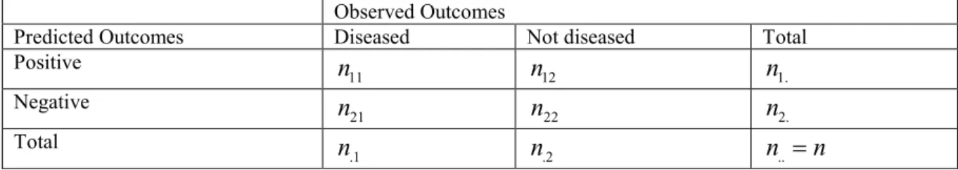
estimated to have actually tested negative to the disease. The resulting four fold contingency table for a given α–prediction rule is Table 1
Table 1: Contingency Table notation for a given
–prediction ruleObserved outcomes Total Predicted outcomes
1
ijy
y
ij
0
,ˆ
ij1
y
a
b
a b
,ˆ
ij0
y
c
d
c d
Totala
c
b d
..n
n
a b c d
Note that a or true positive(TP) is the number of subjects that are observed to have disease
y
ij
1
and predicted to have disease also
y
ˆ
ij,
1
,b or false positive(FP)is the number of subjects that are observed not to have disease
y
ij
0
and predicted to have disease
y
ˆ
ij,
1
,c or false negative(FN)is the number of subjects that are observed to have disease
y
ij
1
and predicted not to have disease also
y
ˆ
ij,
0
,d or true negative(TN)is the number of subjects that are observed not to have disease
y
ij
0
and predicted not to have disease also
y
ˆ
ij,
0
and
n
n
..
a b c d
is the total number of subjects randomly sampled from the population.Based on the results in a classification table 1 for each model, we carry out ROC curve analysis to measure the accuracy of the diagnostic test in discriminating between alternative health status by first calculating the sensitivity and 1-specificity since ROC curve is a graph resulting from the plotting of these values. By varying the value of
in Equation 2.2 between 0 and 1 inclusive, we generate so many predicted outcomes that can be represented inthere corresponding contingency tables for each model. Based on these tables, we calculate values of sensitivity and 1-specificity that will be used in constructing an ROC curve. Specifically here, each α-rule contributes one point to the ROC curve and so since a pair of sensitivity and 1-specificity values contributes one point to the ROC curve, several pairs will be used in constructing a smooth ROC curve. This method of defining AUC represents a shift from the existing works by Buros and Tubbs (2013); Hanley and McNeil (1982) and Mann-Whitney (1947).
CALCULATING AUC BASED ON PREDICTED PROBABILITY OF POSITIVE RESPONSE
To model the AUC based on the contingency table 1, let
y
1ijand y
0ijbe the diagnostic test results of the ithsubject at jth diagnostic test who are drawn randomly from the diseased and non-diseased population respectively while n represents the total number of sampled observations of subjects for those responding positive (diseased)
and negative(non-diseased) from the population, then the AUC is defined as
1 0 1 1 1 0 1 0 1 0 1 0 1 0 1 0 1 11
ˆ
,
,
1, 2,...,
;
1, 2,...,
(
.
)
2.3
1,
,
0.5,
0,
1
ˆ
0.5
2.4
n T ij ij i j ij ij ij ij ij ij ij ij n T ij ij ij ij i jAUC
y
y
i
n subjects j
T diag test
n
where
if y
y
y
y
if y
y
if y
y
Equivalently
AUC
y
y
y
y
n
The AUC defined by equations 2.3 or 2.4 follows the non-parametric MW approach and it is rather flexible and yields ROC estimates even with a better precision than the MW approach or the trapezoidal rule for calculating the AUC. This method of calculating AUC avoids the computational complex procedures of the maximum likelihood estimation (MLE) and numerical integration methods which not only involves lengthy calculations but also have restrictive assumptions about the distribution of diagnostic test results. It is note worthy that estimates from parametric methods such as the method of MLE are inconsistent thereby giving a misleading picture of the regression relationship (Pepe, 2003). Our method of calculating AUC is unique in so many ways: it incorporates predicted probability of positive response in the construction of ROC curve and indeed AUC, it uses the
prediction rule which enables the construction of very smooth ROC curve because several values of
normally will produce smoothness in the curve, the AUC calculated is also diagnostic test dependent since the test result depends on the test for the subjects and finally the method is not only simpler and straight forward but also it avoids the iteration procedure which is rigorous, time consuming and liable to errorrneous results. The new AUC if obtained for two or more diagnostic tests can be compared using a chi-square test statistic proposed for that purpose which approximates continuous distribution to discrete distribution as seen in a contingency table.APPLICATION TO REAL DATA
The proposed methods can be applied to real data on gestational diabetes mellitus(GDM).This was a retrospective study of test results of pregnant women screened using 1 hour 50g Glucose Challenge Test(GCT) and diagnosed using 75g OGTT as well as 100g OGTT according to WHO(1999) and National Diabetic Data Group(NDDG,1979) criteria. These test results were collected using the simple random sampling method. Medical records showed that out of a total of six thousand and ten (6010) pregnant women registered for antenatal clinic (ANC) who were screened using a universal screening with 1 hour 50g Glucose Challenge Test (GCT) for GDM in the sampled hospitals within the two years (from January 2011 to December 2012) chosen for this study, a total sample of 1113 pregnant women who had positive risk factors (such as positive family history of diabetes, age at least 30 years, BMI
30 kg/m2, previous fetal weight
4kg, and positive obstetric history of GDM) and aged between 15-45years at less than 24 weeks and between 24-28 weeks of gestation tested positive for GDM(indicating the presence of GDM) since their plasma blood glucose level was at least 140 mg/dl after 1 hour. These positively responding women were subsequently recalled for confirmatory diagnostic test using 2-hour 75g OGTT in accordance with the criteria set by WHO (1985) and later repeated using 3-hours 100g OGTT during the later part of their gestation period.
The study protocol was according to the recommendations for universal screening by the Fifth International Workshop Conference on Gestational Diabetes (Metzger et al, 2007).The essence of the repeated tests was to actually determine the status of GDM in them. Since the results of the diagnosis are two, one stands the chance of comparing between their tests results (between 2-hours 75g OGTT and 3-hours 100g OGTT). Women who were known diabetics, or who were suffering from any chronic illness were excluded from the study. After obtaining permission from the hospitals’ Research and Ethics Committee, assess was granted into the record units of the antenatal wards of these hospitals where the medical history of the patients were kept in a proforma containing general information on demographic characteristics such as body mass index, maternal age, previous fetal weight and vital clinical histories such as obstetric history of GDM, and family history of diabetes were taken. BMI was calculated by dividing the weight in kilograms by the height in meters squared.
The data for this paper is recorded according to the number of pregnant women, GDM test results (response variable) and their observed risk factors or parent independent variables. This is suitable for fitting the classification models for analysis. Since we have two set of response variable from the two diagnostic tests, we took the average of the test results as observed outcomes. Analysis of this data will yield the predicted probability of positive response needed to be applied in calculating the AUC for the models.
PREDICTED PROBABILITY OBTAINED FROM THE CLASSIFICATION MODELS
We here calculate predicted probability of positive response from the classification models for the purpose of calculating the AUC. Fitting the data to the models, the analysis yielded the results shown in table 2.
Table 2. Predicted probability from the classification models
Classification models Predicted probability p-value F-ratio
Logistic Regression 0.1949 0.0251 10.346
Linear Discriminant Analysis 0.1184 0.0425 6.6421
Dummy variable regression 0.4785 0.0013 15.843
Having obtained the predicted probability of positive response for each of the models as in table 2, we now use each of them to find the predicted outcomes as defined in equation 2.2 as well as the observed outcomes as defined in equation 2.1. Since ROC curve has the ability of evaluating the discriminatory power of a continuous test result (observed outcome) to correctly assign into a two-group classification, the observed outcomes is dichotomized using at least 7.8mmol/l as cut-off value for GDM diagnosis as recommended. Having generated the observed outcomes based on equation 2.1 and predicted outcomes based on equation 3.2, the resulting coded data from these outcomes are cross-classified and will constitute as many tables as contingency table 2.5 for constructing ROC curve for each model. For instance, the contingency table 3 represents a pair of sensitivity and 1-specificity out of 1113 pairs required for constructing the ROC curve for each model.
Table 3. Outcome values for a given
–prediction ruleObserved Outcomes
Predicted Outcomes Diseased Not diseased Total Positive 11
n
n
12n
1. Negative 21n
n
22n
2. Total .1n
n
.2n
..
n
Suppose each α-rule (for instance, table 3) contributes one point to the ROC curve, the estimates of sensitivity and specificity obtained from this table for generating the point is not enough to be used to obtain sufficient pairs of sensitivity and 1- specificity that will enable for the actual smooth ROC curve analysis for each model. In order to have sufficient estimated pairs of sensitivity and 1-specificity that can generate a smooth curve, we vary the
value from 0 to 1 in the prediction rule of equation 2.2 so as to generate multiple prediction rule capable of being used in obtaining enough contingency tables for the construction of ROC curve. This computation is supported by SAS version 9 soft ware. The difference between one model and another model is the predicted probability of positive response for that model. The number of pairs of sensitivity and 1-specificity equals a sample size 1113 for each model. Using this method, the AUCs are obtained for the models.ASSESSING THE DISCRIMINATING ABILITY OF CLASSIFICATION MODELS
Assessment of classification models here is based on their discriminating or predictive ability of diagnostic accuracy. Since many models are available for assessment, interpreting and comparing the models using the ROC curves may be erroneous, instead the interpretation and comparison of the discriminatory accuracy of the test will be based on the AUC which summarizes the accuracy of each model. It is vital to note that these models were chosen because of their similar set of modeling techniques. The estimators of AUC for the selected models are estimated using both parametric and non-parametric methods. From Table 4, result shows that little differences exist among the non-parametric estimates than the parametric estimates. The highest difference in AUC can be seen in linear discriminant analysis. This may be due to its strict compliance to the normality assumption as well as equal variance.
Table 4. CLASSIFICATION MODELS AGAINST METHODS OF CALCULATING AUC
Classification models Binormal parametric mtd(parametric mtd) Predicted probability method (nonparametric mtd) Mann-Whitney U statistic method (nonparametric mtd) Trapezoidal Rule (nonparametric mtd) 1 Logistic Regression 0.6284832 0.6034563 0.6007869 0.6034212 2 Dummy Variable Regression 0.6194562 0.6004383 0.6003231 0.6007853 3 Linear Discriminant Analysis 0.6384753 0.6013955 0.6002135 0.6011457
NORMALITY TEST FOR THE CLASSIFICATION MODELS
The test of normality for the models shows that after estimating maximum likelihood estimate
ˆ
by power transformation, it was discovered that only discriminant analysis is the distribution (Table 5) that have the normal distribution on the basis of the specification of Shapiro-Wilk normality test say at
0.05
. This test suggests that if the chosen alpha level is 0.05 and the p-value is less than 0.05, then the null hypothesis that the data are normally distributed is rejected. If the p-value is greater than 0.05, then the null hypothesis is accepted. Similarly, two test results such as X(diseased) and Y(non-diseased) may not follow normal distribution according to Krzyśko et al (2008), but the fact that parametric binormal ROC curve suggests that two test results such as X(diseased) and Y(non-diseased) must each follow normal distribution always give good results, due to the fact that ROC curves concerns itself with the relationship between distributions instead of the individual distributions.Table 5 Test of Normality for the classification models
GDM STATUS
Diseased=1 Non-diseased=0
ˆ
p-value
ˆ
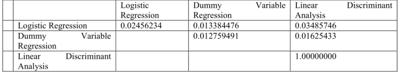
p-value 1 Logistic Regression 1.22 0.0350 1.19 1.05E-26 2 Dummy Variable Regression 0.52 0.0112 0.74 1.03E-04 3 Linear Discriminant Analysis 0.63 0.1064 0.69 2.16E-07Information in cells of Table 6 shows the p-values for the difference between two AUCs when the predicted probability method of calculating AUC is used. The null hypothesis of no difference in AUCs is rejected when any of the p-value is smaller than the level of significance (
0.05
). Table 2.8 showed that the AUCs for linear discriminant analysis did not show any significant difference because the assumptions of normality and equal covariance are not met while dummy variable regression analysis followed by logistic regression analysis showed significant differences in AUCs indicating their flexibility in handling data when the assumption of normality and equal variance is violated.TABLE 6. TESTING THE DIFFERENCE BETWEEN TWO MEASUREMENTS OF AUC USING P-VALUES Logistic Regression Dummy Variable Regression Linear Discriminant Analysis Logistic Regression 0.02456234 0.013384476 0.03485746 Dummy Variable Regression 0.012759491 0.01625433 Linear Discriminant Analysis 1.00000000
SUMMARY AND CONCLUSION
The purpose of this paper was to evaluate the methods of calculating AUC and its significance in assessing classification models. In assessing these classification techniques, it was discovered that non-parametric methods of estimating AUC give convergent results in terms of their measurement for AUC while parametric approaches are known generally for the higher values of AUC. Practically, the assumption of normality cannot be achieved for the parametric methods of estimating AUC. This is why the non-parametric methods are recommended. The strength of our method is that it has easy implementation to discriminate diagnostic test procedures even by non-statisticians. The proposed method offers reliable statistical inferences even in small sample problems and circumvent the difficulties of deriving the statistical moments of complex summary statistics.
DISCUSSION
procedures of the maximum likelihood estimation (MLE) and numerical integration methods which not only involves lengthy calculations but also have restrictive assumptions about the distribution of diagnostic test results since there are parametric methods. It is note worthy that estimates from parametric methods such as the method of MLE are inconsistent thereby giving a misleading picture of the regression relationship (Pepe, 2003). Our method of calculating AUC is unique in so many ways: it incorporates predicted probability of positive response in the construction of ROC curve and indeed AUC, it uses the
prediction rule which enables the construction of very smooth ROC curve because several values of
normally will produce smoothness in the curve, the AUC calculated is also diagnostic test dependent since the test result depends on the test for the subjects and finally the method is not only simpler and straight forward but also it avoids the iteration procedure which is rigorous, time consuming and liable to errorrneous results. Computational burden can still be substantial in binormal ROC curve as a method of calculating AUC because a number of iterative procedures that are involved in obtaining estimators, for instance MLE of AUC (Dorfmann & Alf 1969; Metz et al, 1998).RECOMMENDATIONS
The new method of calculating AUC from predicted probability is recommended because of the reasons given above. It is highly recommended that non-parametric method of calculating AUC such as the predicted probability method be employed because of the fact that it is always distribution free and heavy computational procedures are not required. It is also advised that dummy variable regression be utilized in classifying disease conditions since it not discriminates well, it determines the contributions of the various levels of the parent independent variables.
Acknowledgement
We will not fail to appreciate Dr. Happiness Ilouno of the Department of Statistics, Nnamdi Azikiwe University Awka Nigeria for her encouragement during this research work. Her effort was wonderful.
References
Aoki, K., J. Misumi, T. Kimura, W. Zhao and T. Xie, 1997. Evaluation of cutoff levels for screening of gastric cancer using serum pepsinogens and distributions of levels of serum pepsinogens I, II and of PG I/PG II ratios in a gastric cancer case-control study. Journal of Epidemiology, 7, 143 – 151.
Bamber D. (1975). The area above the ordinal dominance graph and the area below the receiver operating characteristic graph. Journal of Mathematical Psychology 12, 387-415.
Buros, Amy and Tubbs, Jack D.(2013). Applying the Jonckheere-Terpstra Statistic to AUC Regression. Department of Statistical Science, Baylor University, Waco, TX 76706. www.louisville.edu/sphis/bb/srcos-2013/….
DeLong, E.R., DeLong, D.M., Clarke-Pearson, D.L. (1988). Comparing the area under two or more correlated receiver operating characteristic curves: a nonparametric approach. Biometrics 44(3), 837-845.
Dorfman DD, Alf JrE. Maximum likelihood estimation of parameters of signal detection theory and determination of confidence intervals – rating-method data. Journal of Mathematical Psychology 1969; 6: 487-496. D. D. Dorfman and E. Alf, “Maximum likelihood estimation of parameters of signal detection theory: a direct
solution,” Psychometrika, vol. 33, no. 1, pp. 117–124, 1968.
Egan, JP. (1975). Signal detection theory and ROC Analysis. New York: Academic Press.
Green, DM. and Swets, JA. (1966). Signal detection theory and psychophysics. John Wiley & Sons, Inc. New York.
Greiner, M., Pfeiffer, D., and Smith, RD. (2000). Principals and practical application of the Receiver Operating Characteristic analysis for diagnostic tests. Preventive Veterinary Medicine, 45:23–41.
J. A. Hanley and B. J. McNeil, “The meaning and use of the area under a receiver operating characteristic (ROC) curve,” Radiology, vol. 143, no. 1, pp. 29–36, 1982.
Hanley JA, McNeil BJ. A method of comparing the area under two ROC curves derived from the same cases.
Radiology 1983; 148: 839-843.
Hsiao, J. K., J. J. Barko and W. Z. Potter, 1989. Diagnosing diagnoses: receiver operating characteristic methods and psychiatry. Archives of General Psychiatry, 46, 664 – 667.
Krzyśko M., Wołyński W., Górecki T., Skorzybut M. (2008) Systemy uczące się, Wydawnictwo Naukowo-Techniczne
Lasko, T. A., J. G. Bhagwat, K. H. Zou and L. Ohno-Machado, 2005. The Use of Receiver Operating Characteristic Curves in Biomedical Informatics. Journal of Biomedical Informatics, 38, 404 – 415.
L´opez-Rat´on, M., Cadarso-Su´arez, C., and Lado, MJ. (2012a). T´ecnicas de estimaci´on e inferencia de las curvas ROC. Editorial Acad´emica Espa˜ nola.
Mann, H.B & Whitney D.R (1947).On a test whether one of two random variables is stochastically larger than the other.Ann.Math.Statist;18,pp.50-60.
Metz CE. Basic Principles of ROC analysis. Seminars in Nuclear Medicine 1978; 8(4): 283-298. Metz CE. ROC methodology in radiologic imaging. Investigative Radiology 1986; 21(9): 720-733.
Metz, C. E., 1989. Some practical issues of experimental design and data analysis in radiological ROC studies.Investigation Radiology, 24, 234 – 245.
Metzger BE, Buchanan TA, Coustan DR, de Leiva A, Dunger DB, Hadden DR, et al. Summary and recommendations of the fifth international workshop-conference on gestational diabetes mellitus. Diabetes Care 2007; 30: S 251.
Metz, CE., Herman, BA., and Shen, JH. (1998). Maximum likelihood estimation of Receiver Operating Characteristic (ROC) curves from continuously-distributed data. Statistics in Medicine, 17:1033–1053. National Diabetes Data Group. Classification and diagnosis of diabetes mellitus and other categories of glucose
intolerance. Diabetes 1979; 28: 1039–1057
Ogum, G. E. O. (2003). Introduction to methods of multivariate analysis. Afri Towers Ltd. Aba. Nigeria. Okeh U.M and Oyeka I.C.A (2014) Two Factor Analysis of Variance and Dummy Variable Regression Models.
Global Journal of Science Frontier Research: F Mathematics and Decision Sciences. Volume 14 Issue 6 Version 1.0. Online ISSN: 2249-4626 & Print ISSN: 0975-5896.
Okeh U.M and Oyeka I.C.A (2015) One Factor Analysis of Variance and Dummy Variable Regression Models. Global Journal of Science Frontier Research: F Mathematics and Decision Sciences. Volume 15 Issue 7 Version 1.0. Online ISSN: 2249-4626 & Print ISSN: 0975-5896.
Okeh UM and Oyeka ICA (2016). Dummy Variable Multiple Regression Analysis of Matched Samples. Biometrics & Biostatistics International Journal.Volume 3 Issue 5.
Onyeagu, S. I. (2003). A first Course in Multivariate analysis. MegaConcept, Nigeria.
Pepe, M.S. (2003). The statistical evaluation of medical test for classification and prediction. Oxford: Oxford University Press.
Pepe, MS. (2004). The statistical evaluation of medical tests for classification and prediction. 1st ed. Oxford
University Press, USA.
P.K. Sen, On some convergence properties of U statistics, Calcutta Statist. Assoc. Bull. 10 (1960), pp. 1{18. Swets, J. A. and R. M. Picket, 1982. Evaluation of diagnostic systems: methods from signal detection theory.
Academic Press, New York.
WHO. Definition, Diagnosis and Classification of Diabetes Mellitus and its Complications. Report of a WHO consultation. Part 1: Diagnosis and Classification of Diabetes Mellitus. Geneva: Department of Non-communicable Disease Surveillance, World Health Organization, 1999.
Zou, KH., Hall, WJ., and Shapiro, DE. (1997). Smooth non-parametric Receiver Operating Characteristic (ROC) curves for continuous diagnostic tests. Statistics in Medicine, 16:2143–2156.
Zhou, X. H., N. A. Obuchowski and D. K. McClish, 2002. Statistical methods in diagnostic medicine. Wiley, New York.