Genetic Algorithms Applied to Inconsistent Matrices
Correction in the Analytic Hierarchy Process (AHP)
Leonardo S. Wanderer1, Marcelo Karanik1, Diana M. Carpintero1 1Artificial Intelligence Research Group (GISIA)
Universidad Tecnológica Nacional – Facultad Regional Resistencia French 414, Resistencia (3500)
{leonardo.wanderer,dianimax}@gmail.com, [email protected]
Abstract. Making Decision in non-structured problems is not a simple task. For
this reason, decision makers use Decision Support Systems (DSS). These kinds of systems implement techniques and algorithms in order to improve the deci-sion process. Analytic Hierarchy Process (AHP) is one of these techniques which yields a ranking scale of alternatives based on criteria and alternative ma-trices. These matrices make a pairwise comparison between a set of elements compared and must be complete and consistent in order to be processed with AHP. Incompleteness and inconsistency emerge as a consequence of the large data required to be compared by an expert, which exceeds his or her human abilities. Genetic Algorithms (GA) is a powerful used technique which provides simplicity, broad applicability and flexibility for search problems. In this work a GA model is exposed, being its aims to help the expert to fill the matrix and provide reasonable judgments by suggesting possible values.
Keywords: decision making, AHP, genetic algorithms, inconsistency.
1
Introduction
The Analytic Hierarchy Process (AHP) [1] is a general theory, developed by Thomas Saaty, based on pairwise comparisons used to determine priorities of a set of ele-ments. The value assigned to these comparisons could be obtained either by real measurements or by an expert judgment of preference using the fundamental scale proposed by Saaty. AHP is widely used in multi-criteria decision making [2], plan-ning and resource assignment [3], and conflict resolution [4].
Typical decision making problems are characterized by the presence of one or more “experts” who provide their knowledge, many alternatives and many criteria used to evaluate the mentioned alternatives. The available information is processed in order to determine the adequate alternative to solve the problem.
Goal
Criterion 1 Criterion 2 ... Criterion N
Alternative 1 Alternative 2 ... Alternative M
Criterion 3
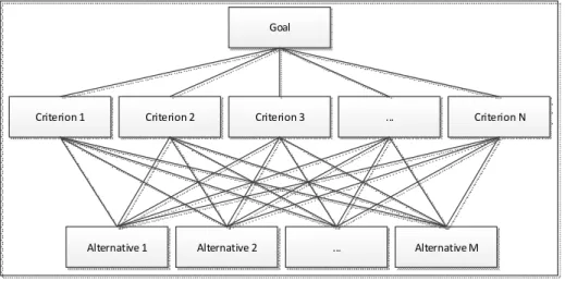
Fig. 1. Hierarchal structure representation.
When the hierarchical structure is built, the expert completes a criteria pairwise comparison matrix using the scale proposed by Saaty. In the same way, comparison matrices for alternatives (one for each criterion) are filled with expert’s preferences.
All mentioned matrices are squared and reciprocal, and their order depends on the number of elements to compare. I.e., for an order matrix the number of comparisons is:
( ) (1) Due to the fact that AHP cannot be used with incomplete matrices, it is necessary to fill all this information. When the number of matrices and elements within them grow, two problems arise: firstly, the large amount of data required to the expert gen-erates tedious data loading process; secondly, the relationship between the compared elements can be inconsistent [5]. The summarization process can only be made after all the comparisons are completed and they are consistent.
The inconsistency can be defined as a mismatch in the value assigned by an expert in the comparison, usually bound to the transitive relationship with other elements. For example, if the relative importance we assign to an element A is more than the assigned to B, and also B is more important than C we would expect that A has much more importance than C. It is more complex to maintain these transitive relationships when the number of elements to compare and the matrix order grow. Saaty proposes a Consistency Ratio (CR) in order to measure the inconsistency level of pairwise matri-ces.
In this work a model to fill incomplete pairwise matrices is presented. Section 2 describes the completeness and consistency problems in AHP. In Section 3 basic con-cepts of Genetic Algorithms are presented. Section 4 introduces the proposed model and Section 5 shows the simulations made and obtained results. Finally, in Section 6 conclusions and Section 7 further work with the genetic algorithm is exposed.
2
Completeness and Consistency in AHP
As mentioned above, AHP has two fundamental requirements for pairwise matrices in order to obtain the priorities of alternatives: completeness and consistency.
Completeness is the easier one because it requires the expert to insert all values in the matrix. Nevertheless, the expert might ignore the exact relationship between the considered elements and, consequently, build inconsistent matrices. Logically, it is desirable that the expert evaluates only those well-known relationships and to deduce the rest based on the transitivity relationship of elements. Clearly, filling those values in this way requires many well-known values already set.
Consequently, consistency requires having other considerations in mind. The pur-pose of consistency check is to guarantee that the judgments are not random or illogi-cal [6]. Since the expert is constrained to the fundamental sillogi-cale and the comparisons are subjectivities, an adequate level of consistency is not easy to obtain. Therefore, Saaty defines a tolerance for the inconsistence equal to 0.1 compared to the consisten-cy ratio (CR) [5], which denotes the actual inconsistenconsisten-cy degree of a matrix. Hence, if this value is less than 0.1, the matrix is consistent enough to obtain an eigenvector (associated to maximum eigenvalue) which represents the relative importance of the compared elements. Otherwise, the matrix needs to be modified whether by an auto-matic or manual method [8].
The is calculated with the following formula:
(2)
where the is the Consistency Index and is the Random Index (which is obtained with the average CI of 500 matrices). The is calculated as follows:
( ) ( ) (3) where the is the maximum matrix’s eigenvalue and is the matrix’s order.
Within the automatic methods we can name the Saaty’s mathematical method [5] and another one which uses neural networks to adjust the matrix values [9]. The ad-vantage of the first method is the simplicity, but its disadad-vantage is the strong modifi-cation of decision maker preferences and the eigenvector tends to change the order of importance of each element. On the other hand, neural networks do not alter radically the valuation but they require a heavy training phase before using. Also, one neural network for each matrix order is required, because they are static structures.
Given the completeness and consistency constraints, we propose a method that merges both advantages from the later exposed methods. This could be achieved de-fining a properly genetic algorithm which considers consistency and the original ex-pert’s valuation. This technique could be useful for correcting and assisting the expert data loading process, and even solving the inconsistency problem.
3
Genetic Algorithms
Genetic Algorithm (GA) is an artificial intelligence technique belonging to the evolu-tionary algorithms group. They are usually used in resources optimization problems and are very useful when there is not a clear heuristic function which defines the strength of a solution. Advantages related to them are the conceptual simplicity, broad applicability, hybridization with other methods, parallelism, and the fact that they are robust to dynamic changes and that they solve problems that have no solution [10].
Genetic algorithms require the definition of two basic elements, the individual structure (or chromosome) and the fitness function. The structure is the representation of a possible solution to the problem. The fitness function assigns the corresponding aptitude value to each individual and guides search among iterations in order to obtain the best solution(s) [10].
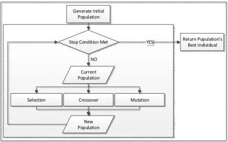
The algorithm is characterized by an iterative process which starts with the creation of a random initial population. This population evolves by using three operators which obtain better individuals that are going to be part of the next population (and replace the previous ones): selection, crossover and mutation [11]. Then, a new itera-tion is made, unless a specific condiitera-tion or set of condiitera-tions are met and the algo-rithms finishes returning the solution(s) [11].
Selection Crossover Mutation
Current Population Generate Initial Population New Population Stop Condition Met
NO
Return Population s Best Individual YES
Fig. 2. Evolutionary Process Overview
4
Proposed Model
Mentioned AHP’s matrix problems could be faced like an operation research optim i-zation problem [12]. The objective is to complete the matrix and preferably alter the smallest number of values, according to the Saaty’s distance [9]. This objective is constrained to the matrix’s inconsistency degree, which must be smaller than 0.1.
Additionally, it is desirable to maintain the importance order of the compared ele-ments (the eigenvector).
Applying this technique to the problem led to an individual structure defined as a vector within an object. This object resembles a wrapper for the structure and offers the services required to evaluate its fitness, expose the underlying matrix and its in-consistency and cloning services among others. The vector structure (see Fig. 3) con-tains an element for each of the r missing values of the original matrix. Many individ-ual objects are contained in the population object which offers another set of services, such as the convergence, the generation (iteration) and the best individual.
Fig. 3.Individual’s structure
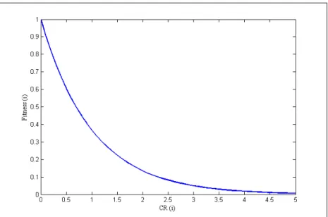
The defined fitness function considers the inconsistency (CR) of the matrix bound to the structure within the individual. For an individual , with an inconsistency ratio ( ), its fitness is defined as shown in the next equation:
( ) ( ) (4) This simple exponential equation makes individuals with high CR to be considered poorly fitted in a similar way. As well as the CR decreases beyond values close to 1, each decrement is considered a much bigger improvement in its fitness.
Defining the structure and the fitness function, the design of the model is described as follows: The process starts with a random population of 150 individuals. Then this population is set as the “current population” and its individuals get through three g e-netic operators: selection, crossover and mutation. The selection causes that an indi-vidual belongs to the next population; the crossover involves a set of indiindi-viduals to interchange their characteristics (i.e. their “genetic material”); and the mutation makes a copy of an individual and induces changes in it, altering its “genetic material”. After that, the new population is checked against the stop condition. This condition contains two exclusive sub-conditions: the first one is met when any individual of the popula-tion has a CR smaller than or equal to 0.1; the second one is an iterapopula-tion threshold (currently set to 100). If these conditions are not met, the process sets the “current population” with the new population and starts a new iteration. Otherwise, the process finishes and returns the best individual of the last obtained population.
The operators and the way in which they are applied, the convergence evaluation methods, the stopping condition, the fitness function and the variation of the mutation probability are parameters for the GA, and can be modified in order to check the ben-efits and drawbacks they induce in the process.
5
Simulations and Results
The main goal is to obtain consistent AHP’s matrices by providing an efficient and unbiased suggesting method for completing and correcting the values in the expert’s comparisons. When the project started, there were defined specific goals in order to achieve the main goal:
Information surveying. GA model design.
Computational module design. Programming.
Testing.
User interface redesign.
Integration between the computational module and the decision support system. Since many of these goals have been already achieved, the goal in progress is “Testing”. These first tests focus on completing the matrix values specifically. After those, it will be defined test for correcting matrices.
The testing set was built with 500 complete matrices for each order from 4 to 9 and for each inconsistency degree: consistent (CR < 0.1), low inconsistency (0.1 ≤ CR < 0.3), medium inconsistency (0.3 ≤ CR < 0.5) and high inconsistency (CR ≥ 0.5). Therefore, three matrices are based on each complete matrix, having respectively 50.00%, 66.66%, and 83.33% of its original values (on the upper diagonal values). Consequently, there are 36000 incomplete matrices in this first testing set.
For this first simulation, the used operators in each phase of the process are: Selection – 10% ─ Elitist Selector Crossover – 85 to 90% ─ Roulette Selector ─ Simple Crossover Mutation – 0 to 5%
─ Uniform Selection (Random) ─ Simple Mutation
─ Percentage: adaptive mutation based on the population’s convergence.
Nevertheless, more operators have been defined, and they will be tested further and compared against this configuration of operators.
The defined model was applied to a set of generated matrices and showed the fol-lowing results:
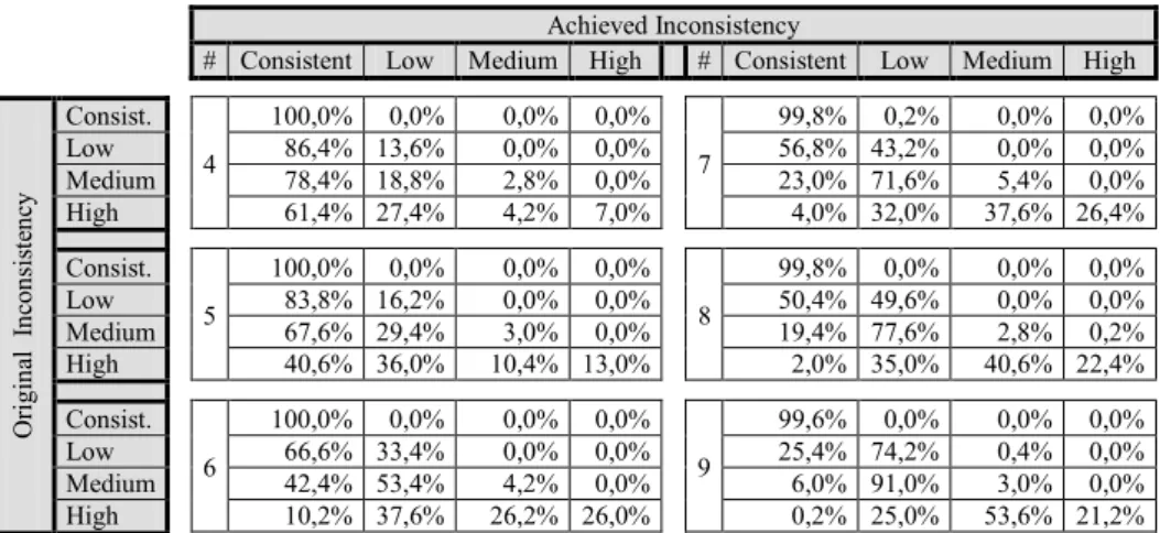
Table 1. Results from 50% complete original matrices.
Achieved Inconsistency
# Consistent Low Medium High # Consistent Low Medium High
O ri gi na l In co nsi st en cy Consist. 4 100,0% 0,0% 0,0% 0,0% 7 99,8% 0,2% 0,0% 0,0% Low 86,4% 13,6% 0,0% 0,0% 56,8% 43,2% 0,0% 0,0% Medium 78,4% 18,8% 2,8% 0,0% 23,0% 71,6% 5,4% 0,0% High 61,4% 27,4% 4,2% 7,0% 4,0% 32,0% 37,6% 26,4% Consist. 5 100,0% 0,0% 0,0% 0,0% 8 99,8% 0,0% 0,0% 0,0% Low 83,8% 16,2% 0,0% 0,0% 50,4% 49,6% 0,0% 0,0% Medium 67,6% 29,4% 3,0% 0,0% 19,4% 77,6% 2,8% 0,2% High 40,6% 36,0% 10,4% 13,0% 2,0% 35,0% 40,6% 22,4% Consist. 6 100,0% 0,0% 0,0% 0,0% 9 99,6% 0,0% 0,0% 0,0% Low 66,6% 33,4% 0,0% 0,0% 25,4% 74,2% 0,4% 0,0% Medium 42,4% 53,4% 4,2% 0,0% 6,0% 91,0% 3,0% 0,0% High 10,2% 37,6% 26,2% 26,0% 0,2% 25,0% 53,6% 21,2%
Table 1 shows that in most of the cases, matrices which belong to a determinate in-consistency range can be improved and can take part of the next more consistent range. The better improvements are shown in the cases when the matrix order is smaller than or equal to 6. It can also be observed that medium inconsistent matrices tend to have better results reducing their CR.
Tables 2 and 3 show a similar behavior as that shown in Table 1. Nevertheless, the reduction in the performance is noticeable. This is due to the fact that improvements are constrained to the number of elements each matrix allows the genetic algorithm to modify. The more complete is the matrix the more constrained is the process to re-duce the inconsistency, and better improvements can be hardly made.
Table 2. Results from 66% complete original matrices.
Achieved Inconsistency
# Consistent Low Medium High # Consistent Low Medium High
O ri gi na l In co nsi st en cy Consist. 4 100,0% 0,0% 0,0% 0,0% 7 100,0% 0,0% 0,0% 0,0% Low 63,2% 36,8% 0,0% 0,0% 13,6% 86,4% 0,0% 0,0% Medium 43,8% 43,4% 12,8% 0,0% 0,4% 71,2% 28,4% 0,0% High 21,0% 33,0% 13,8% 32,2% 0,0% 6,2% 23,6% 70,2% Consist. 5 100,0% 0,0% 0,0% 0,0% 8 99,6% 0,4% 0,0% 0,0% Low 40,0% 60,0% 0,0% 0,0% 9,4% 90,0% 0,6% 0,0% Medium 17,4% 62,4% 20,2% 0,0% 1,2% 69,6% 29,0% 0,2% High 6,4% 25,2% 15,8% 52,6% 0,0% 6,2% 25,4% 68,4% Consist. 6 100,0% 0,0% 0,0% 0,0% 9 99,0% 1,0% 0,0% 0,0% Low 18,6% 81,4% 0,0% 0,0% 4,0% 95,0% 1,0% 0,0% Medium 5,6% 66,6% 27,8% 0,0% 0,8% 74,2% 25,0% 0,0% High 0,4% 10,0% 21,6% 68,0% 0,0% 2,0% 18,2% 79,8%
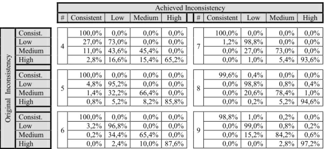
Table 3. Results from 83% complete original matrices.
Achieved Inconsistency
# Consistent Low Medium High # Consistent Low Medium High
O ri gi na l In co nsi st en cy Consist. 4 100,0% 0,0% 0,0% 0,0% 7 100,0% 0,0% 0,0% 0,0% Low 27,0% 73,0% 0,0% 0,0% 1,2% 98,8% 0,0% 0,0% Medium 11,0% 43,6% 45,4% 0,0% 0,0% 27,0% 73,0% 0,0% High 2,8% 16,6% 15,4% 65,2% 0,0% 1,0% 5,4% 93,6% Consist. 5 100,0% 0,0% 0,0% 0,0% 8 99,6% 0,4% 0,0% 0,0% Low 4,8% 95,2% 0,0% 0,0% 0,0% 98,8% 0,8% 0,4% Medium 1,4% 32,2% 66,4% 0,0% 0,0% 20,6% 78,4% 1,0% High 0,8% 5,2% 8,2% 85,8% 0,0% 0,2% 5,2% 94,6% Consist. 6 100,0% 0,0% 0,0% 0,0% 9 98,8% 1,0% 0,2% 0,0% Low 3,2% 96,8% 0,0% 0,0% 0,0% 99,0% 0,8% 0,2% Medium 0,2% 34,4% 65,4% 0,0% 0,0% 15,2% 84,2% 0,6% High 0,0% 2,4% 10,0% 87,6% 0,0% 0,0% 2,8% 97,2%
Additionally, as it was shown in the first table, the medium inconsistent matrices show better results, as well as the matrices with less order.
In all tables the existence of some isolated cases in which the inconsistency got worse can be observed. These cases show that the genetic algorithm requires being adjusted and then tested with other operators for a better performance and for a reduc-tion in these errors.
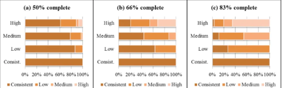
In the graphics below, the decrease in the performance as well as the completeness percentage increases are shown. The predominance of low inconsistent matrices con-sequence as the medium matrices improvements and the unchanged low ones can also be observed.
Fig. 5. Order 4 matrices results.
Fig. 6. Order 5 matrices results.
So forth, many matrices became consistent from each the set. However, this per-formance is not observed with higher matrix order due to having high inconsistency.
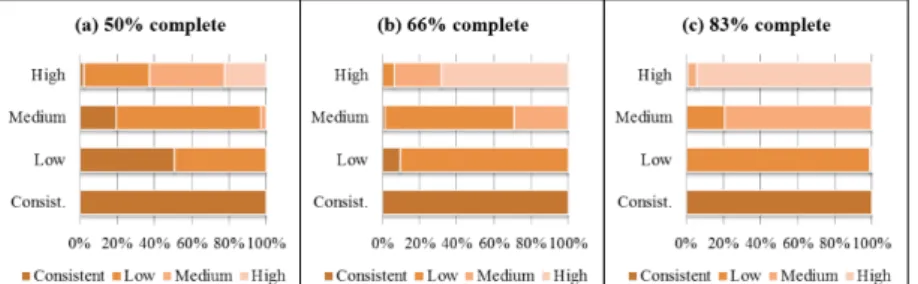
Fig. 9. Order 8 matrices results.
Fig. 10. Order 9 matrices results.
Order 6 and 7 matrices hardly became consistent if they have high or medium in-consistency with more than 50% of its elements complete. Furthermore, in order 8 and 9 matrices with low inconsistency the same behavior is observed.
Additionally, the good performance of the algorithm completing consistent matri-ces and improving inconsistent matrimatri-ces is also noticeable, even though this result decreases while the matrix is more complete, inconsistent and presents a growing order.
6
Conclusions
Summarizing the previous results, four main conclusions can be stated.
First of all, it is easier to reduce inconsistency in medium inconsistent matrices than in high and low ones. As a consequence, there is a predominance of low incon-sistent matrices in the obtained results, being the reasons for this:
Low inconsistent matrices might be inconsistent enough to forbid the genetic algo-rithm to change its values for a better solution.
High inconsistent matrices have such a high CR value that they cannot be modified to reduce it.
Secondly, higher orders of matrices make the inconsistency reduction harder, and most of the matrices just stay in the same inconsistency range as their related com-plete matrices.
Thirdly, the complete percentage has the same effect than the order. The less com-plete matrices provide the genetic algorithm with more freedom degrees in the explo-ration process and, consequently, better solutions are found.
And finally, these first test conclusions reveal the need for a matrix correction which also alters the expert’s original judgments. Some matrices cannot be just co m-pleted in order to achieve a value of 0.1 for the CR due to fact that they are too incon-sistent. It is expected that this situation should hardly arise since the users providing data to AHP are supposed to be experts making decisions in the context of the prob-lem. However, human behavior is very complex and errors under some circumstances should be also expected and have to be fixed. As we stated before, the way we con-sider to be the best is to provide suggestions and let the expert decide if those sugges-tions are what he or she really meant, always trying to alter the judgment already done as little as possible.
7
Further Work
Currently, the genetic algorithm is being adjusted in order to give better results. This also requires trying other genetic operators and make sensitivity analysis over some parameters, such as operator’s usage percentages.
After that, altering the expert’s judgments will be considered during operation, which will also require testing and adjustments as those previously mentioned.
Later, the integration with the DSS will be finally done and the suggesting values module will be ready to provide services to the users of the system.
Furthermore, a sensitivity analysis of eigenvector’s changes will be made in order to compare this technique to the neural networks and Saaty’s correction methods, to see how intrusive its results in the expert’s judgments are.
Acknowledgments. This work has been supported by the project “Design of Tec h-niques for Uncertainty Handling in Multiple Experts Decision Support Systems” UTN-1315 (National Technological University).
References
1. Saaty, R. W.: The analytic hierarchy process - What it is and how it is used. Math Model-ling, Vol. 9, No. 3-5, pp. 161-176 (1987).
2. Triantaphyllou, E., Shu, B., Nieto Sanchez, S., Ray, T.: Multi-Criteria Decision Making: An Operations Research Approach. Encyclopedia of Electrical and Electronics Engineer-ing, (J.G. Webster, Ed.), John Wiley & Sons, New York, NY, Vol. 15, pp. 175-186, (1998).
3. Russell, S., Norvig, P.: Inteligencia Artificial: Un enfoque moderno. Prentice Hall His-panoamericana S.A., México (1996).
6. Kwiesielewicz, M., van Uden, E.: Inconsistent and contradictory judgments in pairwise comparison method in the AHP. Computer & Operations Research 31 pp. 713-719 (2004). 7. Gramajo, S., Karanik, M., Pinto, N., Cabrera, D., Alurralde, M.: Modelo de Apoyo para la
Toma de Decisiones en QoS. CACIC (2011).
8. Gramajo, S., Karanik, M., Cabrera, D., Alurralde, M., Ojeda, P., Pinto, N.: Diseño de Téc-nicas para el Tratamiento de Situaciones de Incertidumbre en Sistemas de Soporte de De-cisiones con Múltiples Expertos. WICC (2012).
9. Gomez-Ruiz, J.A., Karanik, M., Pelaez, J. I.: Estimation of missing judgments in AHP pairwise matrices using a neural network-based model. Applied Mathematics and Compu-tation, Elsevier. Vol. 216(10), pp: 2959-2975. (2010).
10. Sivanandam, S. N., Deepa, S. N.: Introduction to Genetic Algorithms. Springer, Heidel-berg (2008).
11. Goldberg, D. E.: Genetic Algorithms in Search, Optimization and Machine Learning. Ad-dison-Wesley Longman Publishing Co., Boston (1989).