Estimation and inference in univariate and multivariate log-GARCH-X models when the conditional density is unknown

This is a postprint version of the following published document:

Sucarrat,

G

.

,

Grønneberg, S. and

Escribano, A.

(2016).

Estimation and inference in univariate and multivariate

log-GARCH-X models when the conditional density is unknown

.

Computational Statistics & Data Analysis

, v. 100, pp.

582-594.

Available in:

https://doi.org/10.1016/j.csda.2015.12.005

©

Elsevier

This work is licensed under a Creative Commons

Attribution-NonCommercial-NoDerivatives 4.0 International License.

Estimation and inference in univariate and multivariate

log-GARCH-X models when the conditional

density is unknown

Genaro Sucarrat

a,∗

, Steffen Grønneberg

a

, Alvaro Escribano

b

a_{Department of Economics, BI Norwegian Business School, Oslo, Norway} b_{Department of Economics, Universidad Carlos III de Madrid, Madrid, Spain}

Keywords: Log-GARCH-X ARMA-X Multivariate log-GARCH-X VARMA-X Volatility

a b s t r a c t

A general framework forthe estimation and inference in univariate and multivariateGeneralised log-ARCH-X (i.e. log-GARCH-X) models when the conditional density isunknownisproposed.Theframeworkemploys(V)ARMA-Xrepresentationsandrelieson abias-adjustmentinthelog-volatilityintercept.Thebiasisinducedby(V)ARMAestimators,buttheremainingparameterscanbe estimatedinaconsistentandasymptoticallynormalmannerbyusual(V)ARMAmethods.Anestimatorofthebiasandaclosed-form expressionfortheasymptoticvarianceisderived.Addingcovariatesand/orincreasingthedimensionof the model does not change the structure ofthe problem, so the univariatebias-adjustmentprocedureisapplicablenotonlyinunivariatelog-GARCH-Xmodels estimated bytheARMA-Xrepresentation,but also inmultivariatelog-GARCH-Xmodelsestimated byVARMA-Xrepresentations. Extensivesimulationsverifythepropertiesofthelog-momentestimator,andanempiricalapplicationillustratestheusefulnessofthe methods.

1. Introduction

The Autoregressive Conditional Heteroscedasticity (ARCH) class of models due toEngle(1982) is useful in a wide range

of applications. In finance, in particular, it has been extensively used to model the clustering of large (in absolute value) financial returns. Engle himself, however, originally motivated the class as useful in modelling the time-varying conditional uncertainty (i.e. conditional variance) of economic variables in general, and of UK inflation in particular. Other areas of

application include, among others, the uncertainty of electricity prices (e.g.Escribano et al., 2011,Koopman et al., 2007),

the evolution of temperature data (e.g.Franses et al., 2001) and – more generally – positively valued variables, i.e. so-called

Multiplicative Error Models (MEMs), seeBrownlees et al.(2012) for a survey.

Within the ARCH class of models exponential versions are of special interest. This is because they enable richer autore-gressive volatility dynamics (e.g. contrarian or cyclical) compared with non-exponential ARCH models, and because their fitted values of volatility are guaranteed to be positive. The latter is not necessarily the case for ordinary (i.e. non-exponential) ARCH models, particularly when covariates or other conditioning variables (‘‘X’’) are added to the volatility equation. In fact, the greater the dimension of X, the more restrictions are needed in order to ensure positivity. Another desirable property is that volatility forecasts are more robust to jumps and outliers. Robustness can be important in order to avoid volatility

fore-∗_{Correspondence to: Nydalsveien 37, 0484 Oslo, Norway. Tel.: +47 46 41 07 79; fax: +47 23 26 47 88.}

E-mail address:[email protected](G. Sucarrat).

cast failure subsequent to jumps and outliers. The log-GARCH class was independently proposed byPantula (1986);Geweke (1986)andMilhøj(1987).Engle and Bollerslev(1986) argued against log-ARCH models because of the possibility of applying the log-operator (in the log-ARCH terms) on zero-values, which occurs whenever the error term in a regression equals zero.

A solution to this problem, however, is provided inSucarrat and Escribano(2013) for the case where the zero-probability

is zero (e.g. because zeros are due to discreteness or missing values). The solution is only available when estimation is via

the (V)ARMA representation. Finally, two competing classes of exponential ARCH models are the EGARCH (Nelson, 1991)

and the Beta-t-EGARCH model (Harvey, 2013). The former has proved to be much more difficult theoretically (more on this

below), and the latter is not – by its very nature – amenable to the assumption of an unknown conditional density (i.e. the conditional density must be known).

The assumption that the conditional density is unknown is particularly convenient from a practitioner’s point of view. This is because the user then does not need to worry about changing the conditional density from application to application, or alternatively to work with a sufficiently general density that will often make estimation and inference numerically more challenging. This explains the attraction of Quasi Maximum Likelihood Estimators (QMLEs). In the univariate case,

consistency and asymptotic normality of QMLE for GARCH models under mild conditions were first established byBerkes

et al.(2003), andFrancq and Zakoïan(2004). In the exponential case, most of the attention has been directed at the EGARCH,

whose asymptotic properties have turned out to be very difficult to establish, see e.g.Straumann and Mikosch(2006). Only

recently was consistency and asymptotic normality proved (for the univariate EGARCH(1,1) only) under the complicated

condition of continuous invertibility, seeWintenberger(2013). The log-GARCH model is much more tractable.Francq et al.

(forthcoming) prove consistency and asymptotic normality of the Gaussian QMLE for an asymmetric log-GARCH(p

,

q) model under mild conditions. Their method does not employ ARMA representations, which means it is more efficient when the conditional error is normal or close to normal, but not when the conditional density is fat-tailed, see the asymptotic efficiency

comparison inFrancq and Sucarrat(2013). Moreover, the estimator ofFrancq et al.(forthcoming) cannot handle zero-errors

or missing values in the manner suggested bySucarrat and Escribano(2013). Finally,Francq and Sucarrat(2013) propose

an estimator that achieves efficiency for conditional densities that are normal or close to normal, by combining the ARMA-approach with the Centred Exponential Chi-Squared as instrumental QML-density. In the multivariate case, QML results have

been established for the BEKK model ofEngle and Kroner(1995) byComte and Lieberman(2003), for an ARMA–GARCH with

constant conditional correlations (CCCs) byLing and McAleer(2003), for a factor GARCH model byHafner and Preminger

(2009), for a multivariate GARCH with CCCs byFrancq and Zakoïan(2010), and for a multivariate GARCH with stochastic

correlations byFrancq and Zakoïan(2015) under the assumption that the system is estimable equation-by-equation. For

exponential ARCH models there are no multivariate results.Kawakatsu(2006) proposed a multivariate exponential ARCH

model, the matrix exponential GARCH, which contains a multivariate version of the EGARCH model. But there are no proofs for the estimation and inference methods that he proposes.

This paper makes three contributions. It is well-known that all the coefficients apart from the log-volatility intercept in a univariate log-GARCH specification can be estimated consistently (under suitable assumptions) via an ARMA representation,

see for examplePsaradakis and Tzavalis(1999), andFrancq and Zakoïan(2006). However, the estimate of the log-volatility

intercept will be asymptotically biased, and the bias is made up of a log-moment expression that depends on the unknown density of the conditional error. A simple estimator of the log-moment expression made up of the empirical residuals of

the ARMA regression (Section2.2) is derived. The implication of this is that the log-volatility intercept can be estimated

consistently, and hence thatallthe log-GARCH parameters can be estimated consistently via the ARMA representation. An

expression for the asymptotic variance (Section2.3) of the estimator of the log-moment expression is also derived.

In the second contribution of the paper (Section2.4), it is shown that the addition of covariates, i.e. the log-GARCH-X

model, does not alter the relation between the ARMA coefficients and the log-GARCH coefficients. In other words, consistent and asymptotically normal estimation of the ARMA-X representation will produce exactly the same bias as earlier, and so the bias correction procedure described above is applicable also for ARMA-X models. Next, a multivariate log-GARCH-X

model that admits time-varying conditional correlations is proposed (Section3). The model has a VARMA-X representation

with a vector of error-terms. The vector is either IID, which corresponds to the Constant Conditional Correlation (CCC) case, or independent but non-identical (ID), which corresponds to the time-varying correlations case. In both cases, however, each entry in the vector of standardised errors is marginally IID. So the bias-correction from the univariate case can be used equation-by-equation – under suitable assumptions – subsequent to the consistent estimation of the VARMA-X representation.

In the third contribution (Section4) the usefulness of the results is illustrated by means of an application to the modelling

of the uncertainty of electricity prices. Electricity prices are characterised by autoregressive persistence, day-of-the-week effects, large spikes or jumps, ARCH and non-normal conditional errors that are possibly skewed. For robust (to jumps) fore-casts of uncertainty (i.e. volatility) that accommodate all these characteristics, the log-GARCH-X model is particularly suited. The investigation shows that estimated volatility can be substantially biased if sufficient ARCH-lags and day-of-the-week effects are not included.

The rest of the paper is organised as follows. Section2presents the univariate log-GARCH model, the relation between

the univariate log-GARCH model and its ARMA representation, and derives the log-moment estimator and its asymptotic variance. Also, it is shown that the addition of covariates does not alter the relationship between the log-GARCH and ARMA

parameters. Section3shows how the ideas extend to the multivariate case. Section4contains our empirical application,

2. Univariate log-GARCH

The univariate log-GARCH(p

,

q) model is given by

ϵt

=

σt

zt

,

zt

∼

IID

(

0

,

1

),

P

(

zt

=

0

)

=

0

, σt

>

0

,

(1) ln

σ

_t2

=

α

₀

+

p



i=1

αi

ln

ϵ

2_t−i

+

q



j=1

βj

ln

σ

t−j,2 t

∈

_Z

,

(2)

wherepis the ARCH order andqis the GARCH order. In finance,

ϵt

is often interpreted as return or mean-corrected return,

but more generally it is simply the error in a regression model. Throughout, it is assumed that

ϵt

is observable and known. Of

course, this is neither a realistic nor a desirable assumption, but simply reflects the current state of the theoretical literature.

Denotingp∗

=

max{p

,

q

}, if the roots of the lag polynomial 1

−

(α

₁

+

β

₁

)

L

− · · · −

(αp

∗

+

βp

∗

)

Lp

∗

are all greater than 1

in modulus and if

|

E

(

lnz2

t

)

|

<

∞, then ln

σ

t2is stable. For common densities like the Student’stwith degrees of freedom

greater than 2, and the Generalised Error Distribution (GED) with shape parameter greater than 1, then

σ

2

t will generally

be stable as well if ln

σ

_t2is stable. Practitioners are often interested in the dynamics of other powers, e.g. the conditional

standard deviation. For that purpose, it should be noted that thedth power log-GARCH(p

,

q) model can be written as

ln

σ

_td

=

α

_0,d

+

p



i=1

αi

ln

|

ϵt−i

|

d

+

q



j=1

βj

ln

σ

t−j,d d

>

0

,

(3)

where

α

0,d

=

α

0d

/

2. This means a complete analysis of thedth power log-GARCH model can be undertaken in terms of the

d

=

2 representation.

2.1. The ARMA representation

If

|

E

(

lnz2_t

)

|

<

∞, then the log-GARCH(

p

,

q) model(1)–(2)admits the ARMA(p

,

q) representation ln

ϵ

_t2

=

φ

₀

+

p



i=1

φi

ln

ϵ

_t−i2

+

q



j=1

θj

ut−j

+

ut

,

ut

=

lnzt2

−

E

(

lnz2t

),

(4) where

φ

0

=

α

0

+



1

−

q



j=1

βj



·

E

(

lnz_t2

),

φi

=

αi

+

βi

and

θj

= −

βj.

(5) Consistent and asymptotically normal estimates of all the ARMA parameters – and hence all the log-GARCH parameters

except the log-volatility intercept

α

0– are thus readily obtained via usual ARMA estimation methods subject to appropriate

assumptions, see e.g.Brockwell and Davis(2006). To estimate

α

0, the most common solutions have been to either impose

restrictive assumptions regarding the distribution ofzt(say, normality, see e.g.Psaradakis and Tzavalis(1999)), or to use an

ex postscale-adjustment (see e.g.Bauwens and Sucarrat, 2010, andSucarrat and Escribano, 2012). What is shown below is

that theex postscale-adjustment (i.e. formula(6)and its modified version(8)) provides a consistent estimate ofE

(

lnz2

t

)

.

Consequently, the final log-GARCH parameter

α

0can also be estimated consistently.

2.2. On consistency

The scale-adjustment employed byBauwens and Sucarrat(2010), andSucarrat and Escribano(2012), is essentially a

smearing estimate (more on this below). Consider writing(1)as

ϵt

=

σ

_t∗z_t∗

,

z_t∗

∼

IID

(

0

, σ

_z2∗

),

where

σ

_t∗is a time-varying scale, not necessarily equal to the standard deviation, and wherez_t∗does not necessarily have

unit variance. Of course, by construction

σt

=

σ

∗

t

σz

∗ andzt

=

zt∗

/σz

∗. Next, suppose a log-scale specification (e.g. an

ARMA specification contained in(4)) is fitted to ln

ϵ

_t2, with ln

_

σ

_t∗2denoting the fitted value of the ARMA specification such

that

_

σ

∗

t

=

exp

(

ln



σ

∗

t

)

, and with the ARMA residual defined as



ut

=

ln

ϵ

2

t

−

ln



σ

∗2

t . In order to obtain an estimate of the

time-varying conditional standard deviation, which is needed for comparison with other volatility models, then it is natural

to consider adjusting

_

σ

∗

t by multiplying it with an estimate of

σz

∗, say, the sample standard deviation of the standardised

residuals



z

∗

t. Although this argument is fine heuristically, it is not straightforwardly apparent what underlying magnitude

the adjustment actually estimates. It transpires that, in the log-GARCH model, the log of the scale-adjustment provides an

estimate of

−

E

(

lnz2_t

)

. To see this, consider the scale adjustment and its approximation:



σ

2 z∗

=

1 T

−

1 T



t=1

(



z ∗ t

−



z ∗ t

)

2

_≈

1 T T



t=1

(



z ∗ t

)

2

₌

1 T T



t=1 exp

(



ut

).

The population analogue of the final expression isE

[exp

(

ut

)

]. Taking the natural log of

E

[exp

(

ut

)

]

gives lnE

[exp

(

ut)

] =

−

E

(

lnz2

t

)

under the assumption thatE

(

zt2

)

=

1, i.e. the identifiability assumption from(1). This suggests that

−

ln



1 T T



t=1 exp

(

_

ut)



(6)

provides a consistent estimate ofE

(

lnz2

t

)

, due to the continuity of the logarithm function.

The expression in square brackets in(6), i.e.T−1



t=Texp

(



ut

)

, is well-known as the ‘‘smearing estimate’’, seeDuan

(1983). It provides an estimate of the adjustment needed for an unbiased estimate ofE

(

yt

|

xt

)

when the left-hand side of

the estimated model is lnyt. The proof ofDuan(1983), however, is for static models. In dynamic models, e.g. when the



ut’s

are ARMA residuals, then a different proof strategy and additional assumptions are needed. Complete proofs under mild assumptions that hold under all the configurations covered in this paper, however, are beyond our scope. For simplicity and convenience, therefore, a set of minimal assumptions and conditions relied upon throughout is formulated, and a proof

of the key condition (A2) is provided only in the log-ARCH(p) case (recently,Francq and Sucarrat(2015) prove A2 for an

equation-by-equation least squares estimator of a multivariate log-GARCH-X model with Dynamic Conditional Correla-tions).

Formally, the following assumptions are relied upon: A1:E

(

z2

t

)

=

1 and

|

E

(

lnzt2

)

|

<

∞.

A2: Let



ut,t

=

1

, . . . ,

Tdenote the ARMA-residuals resulting from estimating the ARMA representation(4). Then:

1 T T



t=1 exp

(

_

ut

)

−

1 T T



t=1 exp

(

ut

)

=

oP(1

).

(7)

In A1, the first moment condition is simply the identifiability condition from(1), whereas the other moment condition

|

E

(

lnz_t2

)

|

<

∞

is required for the ARMA representation(4)to exist. For the two most commonly used densities ofzt in

finance, i.e.N

(

0

,

1

)

andt,E

(

lnz_t2

)

are finite. Regarding A2, it immediately implies that(6)is a consistent estimator ofE

(

lnz_t2

)

due to the continuity of the logarithm function. As already noted, though, a complete proof of A2 under all the configurations

covered by this paper is beyond our scope. In the log-ARCH(p) case, however, the proof is relatively straightforward.

Theorem 1.Supposeln

σ

2

t

=

α

0

+



p i=1

αi

ln

ϵ

2

t−iin(1)–(2), that ln

ϵ

2t is strictly stationary and that A1holds. The

mean-corrected AR(p) representation is then given by

(

ln

ϵ

2

t

−

E

(

ln

ϵ

t2

))

=



p

i=1

φi(

ln

ϵ

t−i2

−

E

(

ln

ϵ

2t

))

+

ut, where

φi

=

αi

as

in(5). Define



Yt

=

ln

ϵ

t2

−

T −1



T

t=1ln

ϵ

t2. Let



φ

1

, . . . ,



φp

denote the OLS estimates of

φ

1

, . . . , φp

based on the



Yt’s, let



ut

=



Yt

−



p

i=1



φi



Y_t−ifor t

>

p and let

_

u_t

=

0for0

<

t

≤

p. If E

(

z_t4

) <

∞

and

|

E

[

(

lnz_t2

)

2

]|

<

∞

, thenA2holds.

Proof. SeeAppendix A.

The theorem states that A2 holds when the mean-corrected AR(p) representation of a log-ARCH(p) model is estimated

by OLS, which then implies that(6)is a consistent estimator ofE

(

lnz2

t

)

. Next, it follows straightforwardly that all the

log-ARCH(p) parameters can be estimated via the relationships in(5), since



φ

0

=

(

1

−



p

i=1



φi)

·

T−1



T

t=1ln

ϵ

2t provides

a consistent estimate of

φ

0under the assumptions of the theorem. Strict stationarity of ln

ϵ

t2follows if the roots of the

AR-polynomial are all outside the unit-circle.

2.3. On normality

Our main interest is a consistent estimator ofE

(

lnz2

t

)

, so that the ARMA-estimates can be used to consistently estimate

all the log-GARCH parameters via the relationships in(5). To this end, the limiting distribution of the estimator ofE

(

lnz_t2

)

is of minor interest. In simulations, however, the limiting distribution and an expression for the asymptotic variance can be useful in verifying simulation results.

Let(6)be modified to



τT

= −

ln



1 T T



t=1 exp

(



ut

−



uT)



,

(8)

where



uTis the empirical mean of the ARMA-residuals. The mean-correction term



uTis needed, since asymptotic normality

may not be achieved without it. See e.g. the related discussion inYu(2007), where high moment partial sum processes of

residuals in ARMA models are treated, and where a mean-correction term is needed for asymptotic normality. In some cases,

e.g. when OLS is used to estimate the AR(p) representation of a log-ARCH(p) model, then



uTis zero by construction, and so

A3: Let

{

_

ut

}

Tt=1denote the ARMA-residuals resulting from estimating the ARMA representation(4). Denoting



uTanduTas

the averages of

_

utandut, respectively:

√

T



1 T T



t=1 exp

(

_

ut

−



uT)

−

1 T T



t=1 exp

(

ut

−

uT)



=

oP(1

).

A4: E

(

z4 t

) <

∞

and

|

E

[

(

lnzt2

)

2

]|

<

∞.

Condition A3 is slightly stronger than A2, since A3 implies that(8)provides a consistent estimate ofE

(

lnz2

t

)

as long as A1

holds. The moment conditions inA4 are needed for the asymptotic variance of(8)to be finite.

Theorem 2. Suppose(1)–(2),A1,A3andA4hold. Then

√

T



_

τT

−

E

(

lnz_t2

)



−→

D N

(

0

, ζ

2

),

where

ζ

2

=

Var

(

z_t2

−

lnz_t2

).

(9)

Proof. SeeAppendix B.

The key assumption for asymptotic normality to hold is A3, but a complete proof under all the configurations covered

by this paper is beyond our scope. Just as for consistency in the log-ARCH(p) case (seeTheorem 1), however, a proof of

asymptotic normality is relatively straightforward.

Theorem 3. Suppose the assumptions of Theorem1hold. If in addition E

(

u4

t

) <

∞

, thenA3holds.

Proof. SeeAppendix A.

Assumption A4 holds under the assumptions ofTheorem 1. The conditionE

(

u4

t

) <

∞

is, in fact, a very weak additional

assumption, since it follows from E

(

e|ut|

_{) <}

_{∞. An extensive set of Monte Carlo simulations have been performed,}

of which a small subset is available as supplementary material from the Webpage of the first author (available as

http://www.sucarrat.net/research/lgarchxsims.pdf). The simulations confirm that the usual ARMA-methods (e.g. Nonlinear Least Squares and Gaussian QML) provide consistent estimates, and that the empirical standard errors coincide with their asymptotic counterparts.

2.4. Log-GARCH-X

Additional covariates or conditioning variables (‘‘X’’) can be added linearly or nonlinearly to the log-volatility specification ln

σ

2

t without affecting the relationship between the log-GARCH coefficients and the ARMA coefficients. Specifically, let the

log-GARCH-X model be given by

ln

σ

_t2

=

α

₀

+

p



i=1

αi

ln

ϵ

2_t−i

+

q



j=1

βj

ln

σ

_t−j2

+

g

(λ,

xt

),

(10)

whereg is a linear or nonlinear function of the conditioning variablesxtand a parameter vector

λ

. The indextinxtdoes

not necessarily mean that all (or any) of its elements are contemporaneous. If

|

E

(

lnz_t2

)

|

<

∞, then

(10)admits the ARMA-X

representation ln

ϵ

_t2

=

φ

₀

+

p



i=1

φi

ln

ϵ

_t−i2

+

q



j=1

θj

ut−j

+

g

(λ,

xt)

+

ut

,

ut

=

lnz2t

−

E

(

lnz 2 t

),

(11)

where the ARMA coefficients are defined as before, i.e. by(5). A complete proof of consistency and asymptotic normality

would of course require precise assumptions on the behaviour ofxt, see for exampleFrancq and Sucarrat(2015), and Chapter

4 inHannan and Deistler(2012).

One type of conditioning variable that is of special interest in financial applications is leverage or volatility asymmetry.

Table 1provides simulation results for a simple version of leverage,g

(λ,

xt

)

=

λ

1I{zt−1<0}, whereI{zt−1<0}is an indicator

function equal to 1 ifzt−1

<

0 and 0 otherwise. Note thatI{zt−1<0}is observable, sinceI{zt−1<0}

=

I{ϵt−1<0}. The simulations

show that all the parameters are estimated consistently, and the second-to-last column shows that the finite sample

empirical standard error of the estimate ofE

(

lnz2_t

)

corresponds well to its asymptotic counterpart (last column), both for

Table 1

Finite sample properties of the LSE via the ARMA representation for a log-GARCH(1,1) with leverage.

DGP T m(α0) se(α0) m(α1) se(α1) m(β1) se(β1) m(λ1) se(λ1) m(τ) se(τ) ase(τ) A: 500 −0.056 0.146 0.098 0.034 0.765 0.124 0.001 0.138 −1.272 0.078 0.067 1000 −0.021 0.079 0.099 0.023 0.785 0.065 −0.011 0.088 −1.271 0.054 0.054 2000 −0.011 0.048 0.099 0.016 0.795 0.041 −0.008 0.063 −1.270 0.039 0.038 B: 500 −0.101 0.271 0.050 0.032 0.830 0.198 −0.019 0.131 −1.271 0.078 0.067 1000 −0.035 0.101 0.050 0.019 0.877 0.073 −0.016 0.079 −1.273 0.054 0.054 2000 −0.013 0.045 0.050 0.012 0.891 0.039 −0.021 0.044 −1.270 0.038 0.038 C: 500 −0.064 0.157 0.099 0.035 0.756 0.132 −0.013 0.142 −1.384 0.086 0.085 1000 −0.023 0.079 0.100 0.023 0.784 0.064 −0.010 0.094 −1.392 0.060 0.061 2000 −0.009 0.050 0.100 0.016 0.793 0.039 −0.010 0.065 −1.391 0.043 0.043 D: 500 −0.099 0.251 0.049 0.030 0.841 0.173 −0.020 0.137 −1.394 0.092 0.085 1000 −0.038 0.119 0.050 0.018 0.874 0.090 −0.027 0.078 −1.392 0.061 0.061 2000 −0.016 0.051 0.050 0.013 0.889 0.040 −0.022 0.049 −1.390 0.045 0.043 The estimated model is lnσ2

t =α0+α1lnϵt2−1+β1lnσt2−1+λ1I{zt−1<0}. DGP A:(α0, α1, β1, λ1, τ)=(0,0.1,0.8,−0.01,−1.27)withzt ∼N(0,1).

DGP B:(α0, α1, β1, λ1, τ) = (0,0.05,0.9,−0.02,−1.27)withzt ∼ N(0,1). DGP C:(α0, α1, β1, λ1, τ) = (0,0.1,0.8,−0.01,−1.39)withzt ∼

standardised t(10). DGP D:(α0, α1, β1, λ1, τ)=(0,0.05,0.9,−0.02,−1.39)withzt ∼standardised t(10).m(x), sample mean of the estimatex.se(x),

sample standard deviation (division byRinstead ofR−1, whereR=1000 is the number of replications).ase(τ), asymptotic standard error ofτ(computed

asζ2_/√_{T, whereζ}2_{is given inTheorem 2). Computations inR(R Core Team, 2014) with thelgarchpackage version 0.2 (Sucarrat, 2014).} 3. Multivariate log-GARCH

TheM-dimensional log-GARCH model is given by

ϵt

∼

ID

(

0

,

Ht), t

∈

_Z

,

(12) D2_t

=

diag



σ

_m2_,t



,

m

=

1

, . . . ,

M

,

(13) zt

=

D−t1

ϵt

,

∀

m

:

zm,t

∼

IID

(

0

,

1

),

P

(

zt

=

0

)

=

0

,

(14) ln

σ

_t2

=

α

₀

+

p



i=1

αi

ln

ϵ

_t−i2

+

q



j=1

βj

ln

σ

t−j,2 p

≥

q

,

(15) where

ϵt

,

σ

2

t andztareM

×

1 vectors, and whereHtandDtareM

×

Mmatrices. In(15)we have that

α

0

=

(α

1.0

, . . . , αM

.0

)

′,

αi

=







α

11.i

· · ·

α

1M.i

... ... ...

αM

1.i

· · ·

αMM

.i







and

βj

=







β

11.j

· · ·

β

1M.j

... ... ...

βM

1.j

· · ·

βMM

.j







,

(16)

where′is the transpose operator. Eq.(12)means that

ϵt

is independent with mean zero and a time-varying conditional

covariance matrixHt. The IID assumption in Eq.(14)states that each marginal series

{

zm,t

}

isIID

(

0

,

1

)

. Marginal identicality is

a key characteristic of the ARCH class of models, and is needed for(6)(or(8)) to be applicable after estimation via the VARMA

representation. An implication of(14)is thatzt

∼

ID

(

0

,

Rt

)

, whereRtis both the conditional covariance and correlation

matrix – possibly time-varying – ofzt. In other words, the vectorztis ID, but not necessarily IID, even though each marginal

series

{

zmt

}

is IID. In the special case where vectorzt is IID, thenRt is a Constant Conditional Correlation (CCC) model.

Estimation of the volatilitiesD2

t does not require that the off-diagonals ofHt(i.e. the covariances) are specified explicitly.

Nor need we assume that

ϵt

is distributed according to a certain density, say, the normal.

3.1. The VARMA representation

If

|

E

(

lnz2

t

)

|

<

∞, then the

M-dimensional log-GARCH(p

,

q) model(15)admits the VARMA(p

,

q) representation

ln

ϵ

_t2

=

φ

₀

+

p



i=1

φi

ln

ϵ

_t−i2

+

q



j=1

θj

ut−j

+

ut

,

ut

=

lnz2t

−

E

(

lnzt2

),

(17) where

φ

0

=

α

0

+



IM

−

q



j=1

βj



·

E

(

lnz_t2

),

φi

=

αi

+

βi,

and

θj

= −

βj.

(18)

In the special case where vectorztis IID, which implies a CCC model for the correlations (assuming they exist), then vector

utis IID as well. In this case, it is well-known that the multivariate Gaussian QMLE provides consistent and asymptotically

normal estimates of the VARMA coefficients under suitable assumptions, see e.g.Lütkepohl(2005). Accordingly, consistent

Table 2

Finite sample properties of equation-by-equation Gaussian QML of a 2-dimensional log-GARCH(1,1) w/diagonal matrixβ1when the correlations follow the DCC ofEngle(2002). DGP T m(α10) m(α20) m(α11) m(α21) m(α12) m(α22) m(β11) m(β22) m(τ1) se(τ1) m(τ2) se(τ2) ase(τ) A: 1 000 −0.065 −0.229 0.046 0.101 0.101 0.048 0.902 0.680 −1.270 0.056 −1.270 0.054 0.054 5 000 −0.013 −0.042 0.049 0.100 0.100 0.049 0.900 0.697 −1.271 0.024 −1.270 0.023 0.024 10 000 −0.005 −0.023 0.049 0.100 0.100 0.050 0.900 0.698 −1.271 0.017 −1.270 0.017 0.017 B: 1 000 −0.029 −0.026 0.098 0.053 0.053 0.097 0.791 0.792 −1.270 0.055 −1.268 0.053 0.054 5 000 −0.005 −0.004 0.100 0.051 0.050 0.099 0.799 0.799 −1.270 0.024 −1.270 0.024 0.024 10 000 −0.003 −0.002 0.100 0.050 0.050 0.100 0.799 0.799 −1.269 0.017 −1.271 0.017 0.017 The estimated model is lnσ2

t =α0+α1lnϵt2−1+β1lnσt2−1, whereα0=(α10, α20)′,α1= 

α11 α12 α21 α22 

andβ1=diag(β11, β22). The standardised errors (z1t,z2t)′are governed by the DCC ofEngle(2002):(z1t,z2t)′∼N(0, Σt),Σt=

 1 ρt ρt 1  ,ρt=q12,t/ √ q1,tq2,t,q12,t=ρ+a(z1,t−1z2,t−1−ρ)+b(q12,t−

ρ),q1,t=1+a(z21,t−1−1)+b(q1,t−1),q2,t=1+a(z22,t−1−1)+b(q2,t−1)witha=0.05 andb=0.9. Estimation proceeds in three steps (the DCC

is not estimated). First, a univariate ARMA-X specification is fitted to each of the two equations with the Gaussian QMLE. Second, the ARMA-X residuals

u1tandu2t, respectively, are used equation-by-equation to estimateτ1andτ2, respectively, with formula(8). Finally, the ARMA-X estimates andτ1and τ2are combined using the relationships in(18)to obtain the log-GARCH estimates.m(x), sample mean of the estimatex.se(x), sample standard deviation

(division byRinstead ofR−1, whereR=1000 is the number of replications).ase(x), asymptotic standard error ofx(computed as√av(x)/√T, where

av(τ1)=av(τ2)=ζ 2_{, seeTheorem 2). In DGP A:α} 1 =c(0,0)′,α1=  0.05 0.10 0.10 0.05  ,β1=diag(0.90,0.70)andρ = −0.2. In DGP B:α1=c(0,0)′, α1=  0.10 0.05 0.05 0.10 

,β1=diag(0.80,0.80)andρ=0.4. Computations inR(R Core Team, 2014) with thelgarchpackage version 0.2 (Sucarrat, 2014).

intercept

α

0– are available as well. In order to obtain a consistent estimate of

α

0, then an estimate of theM

×

1 vector

E

(

lnz2

t

)

is needed. Since the process

{

um,t

}

is marginally IID for eachm, equation-by-equation application of(6)(or of(8))

after estimation of the VARMA can be used to estimate each element inE

(

lnz2_t

)

.

In the case where vector zt is only ID, which is implied by time-varying correlations, then vectorut is only ID as

well. This corresponds to a VARMA model with heteroscedastic errorut. Fewer QML results are available in this case, e.g.

Bardet and Wintenberger(2009). However, in the special case where the

βj

matrices are diagonal, then theM-dimensional

VARMA model can be estimated equation-by-equation (along the lines ofFrancq and Zakoïan(2015)) by univariate ARMA-X

methods, since – equation-by-equation – each error termum,tis IID. Next, equation-by-equation application of(6)provides

an estimate of each element inE

(

lnz2

t

)

, and hence of the log-volatility intercept

α

0.Table 2contains simulation results of

the case where the correlations are governed by the Dynamic Conditional Correlations (DCC) model ofEngle(2002). The

finite sample bias tends to zero asTincreases, and the last two columns show that the empirical sample standard errors

coincide with their asymptotic counterparts as implied by(9). Additional simulations are available from the Webpage of the

first author (available ashttp://www.sucarrat.net/research/lgarchxsims.pdf).

3.2. Multivariate log-GARCH-X

Just as in the univariate case, the multivariate log-GARCH model permits additional covariates or conditioning variables

in each of theMequations. Specifically, write the multivariate log-GARCH-X specification as

ln

σ

_t2

=

α

₀

+

p



i=1

αi

ln

ϵ

2_t−i

+

q



j=1

βj

ln

σ

_t−j2

+

λ

xt

,

(19)

wherextis anL

×

1 vector of covariates, and where

λ

is anM

×

Lmatrix. For notational economy, the covariatesxtenter

linearly, but in principle they can enter non-linearly as in the univariate case, see(11). Similarly, indext inxt does not

necessarily mean that all (or any) of its elements are contemporaneous. The VARMA-X representation of(19)is then given by

ln

ϵ

_t2

=

φ

₀

+

p



i=1

φi

ln

ϵ

_t−i2

+

q



j=1

θj

ut−j

+

λ

xt

+

ut,

with the VARMA coefficients andutdefined as before, i.e. by(18). In other words, the relation between the VARMA

coeffi-cients and the log-GARCH coefficoeffi-cients are not affected by adding

λ

xtto(19). So VARMA-X methods can be used to estimate

all the log-GARCH parameters (under suitable assumptions onxt) except the log-volatility intercept

α

0in a first step, and

then in a second step equation-by-equation application of(6)can be used to estimate each element inE

(

lnz_t2

)

and, hence,

the log-volatility intercept

α

0. Also here it is useful to distinguish between the CCC and time-varying correlations cases. Ifut

is IID, i.e. the CCC case, then – under suitable assumptions – the multivariate Gaussian QMLE provides consistent estimates

of the VARMA-X representation, see e.g.Hannan and Deistler(2012). If correlations are time-varying, and if the matrices

βj

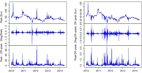
are diagonal, then each equation can be estimated separately in terms of their ARMA-X representations, seeFrancq and

Fig. 1. Daily peak and off-peak spot electricity prices (and their nominal and relative differences) in Euros per MW/h, and log-returns for the Oslo area in Norway, 1 January 2010–20 May 2014 (1601 observations before lag-adjustments).

4. Application: Modelling the uncertainty of electricity prices

Daily electricity prices are characterised by autoregressive persistence, day-of-the-week effects, large spikes or jumps,

ARCH and non-normal conditional errors that are possibly skewed.Koopman et al.(2007),Escribano et al.(2011), and

Bauwens et al.(2013) have proposed univariate and multivariate models that contain some or several of these features. However, in none of these models is the volatility specification – a non-exponential GARCH – robust to the large spikes that are a common characteristic of electricity prices. Nor, are they flexible enough to accommodate a complex and rich heteroscedasticity dynamics similar to that of the mean specification without imposing very strong parameter restric-tions (e.g. non-negativity). Finally, automated model selection with a large number of variables is infeasible in practice due to computational complexity and positivity constraints. The log-GARCH-X class of models, by contrast, remedies these deficiencies.

The data consist of the daily peak and off-peak spot electricity prices (in Euros per kW/h) from 1 January 2010 to 20 May 2014 (i.e. 1601 observations before lag-adjustments) for the Oslo region in Norway. The source of the data is

http://www.nordpoolspot.com/, and the sample was determined by availability: Observations prior to the sample period are not available, and the data were downloaded just after 20 May 2014. Electricity forwards for this region are traded at the Nord Pool Spot energy exchange, a leading European market for electrical energy. Factories, companies and other institutions with electricity consumption may want to shift part of their activity to and from peak hours for efficient cost management, since the difference between peak and off-peak prices can be very large at times, see the bottom graphs of

Fig. 1. As an aid in the decision-making process, forecasts of future prices and of price uncertainty (i.e. volatility or risk) can,

therefore, be of great usefulness. The daily peak spot priceS1,tis computed as the average of the spot prices during peak

hours, i.e.S1,t

=

(

St(8 am)

+ · · · +

St(9 pm)

)/

14, whereas the daily off-peak spot priceS2,tis computed as the average of the

spot prices during off-peak hours, i.e.S2,t

=

(

St(0 am)

+ · · · +

St(7 am)

+

St(10 pm)

+

St(11 pm)

)/

10. Note thatSt(8 am)should

be interpreted as the electricity price from 8 am to 9 am,St(9 am)should be interpreted as the electricity price from 9 am

to 10 am, and so on. Graphs ofS1,t,S2,tand their log-returns (rt

=

∆lnSt) are contained inFig. 1. The price and returns

figures exhibit the usual characteristics of electricity prices, namely that the price variability is substantially larger than the variability of, say, stock prices, stock indices and exchange rates, and that big jumps occur relatively frequently.

The conditional mean is specified as a two-dimensional Vector Error Correction Model (VECM) augmented with day-of-the-week dummies in both equations (the R-squared of the two equations are 0.26 and 0.17, respectively; more details are available on request). The residuals or mean-corrected returns from the estimated model are then used for the estimation of the log-volatility specifications. The univariate models of the two mean-corrected returns are

log-GARCH-1

:

ln

σ

_t2

=

α

₀

+

α

₁ln

ϵ

_t−2₁

+

β

₁ln

σ

_t−2₁

,

(20) log-GARCH-2

:

ln

σ

_t2

=

α

₀

+

7



i=1

αi

ln

ϵ

_t−i2

+

β

₁ln

σ

_t−2₁

,

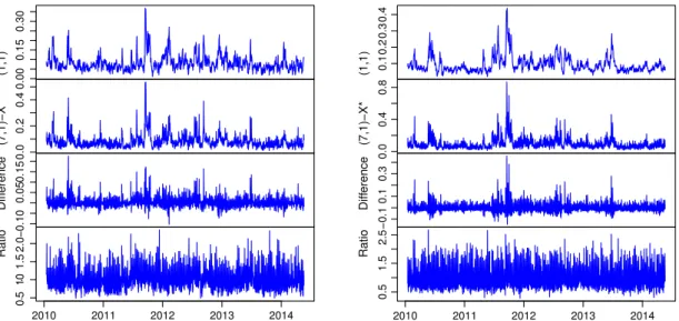
(21)

Fig. 2. Fitted standard deviations (SDs) of the univariate log-GARCH-1 and log-GARCH-4 models, and the nominal differences and ratios between the SDs (computed as log-GARCH-4 minus log-GARCH-1 and log-GARCH-4 over log-GARCH-1, respectively).

log-GARCH-3

:

ln

σ

_t2

=

α

₀

+

7



i=1

αi

ln

ϵ

_t−i2

+

β

₁ln

σ

_t−2₁

+

6



l=1

λl

xlt

,

(22) log-GARCH-4

:

ln

σ

₁2_t

=

α

₀

+

7



i=1

α

1.iln

ϵ

12,t−i

+

7



i=1

α

2.iln

ϵ

22,t−i

+

β

1ln

σ

12,t−1

+

6



l=1

λl

xlt

,

(23) log-GARCH-5

:

ln

σ

₁2_t

=

α

₀

+

7



i=1

α

1.iln

ϵ

12,t−i

+

7



i=1

α

2.iln

ϵ

22,t−i

+

6



l=1

λl

xlt

,

(24)

where

ϵt

is the mean-corrected return in question, and wherex1t, . . . ,x6tare six day-of-the-week dummies for Tuesday

to Sunday. In the last two specifications,

ϵ

2,t is the mean-corrected off-peak return when

ϵ

1,t is the mean-corrected

on-peak return, and vice-versa,

ϵ

2,tis the mean-corrected on-peak return when

ϵ

1,tis the mean-corrected off-peak return. Of

course, this means that the last two equations could be considered as an equation-by-equation estimation scheme similar

to that ofFrancq and Zakoïan(2015), except that we do not estimate the time-varying correlations. The last specification, i.e.

log-GARCH-5, actually refers to a more parsimonious version than the one displayed. The parsimonious specification

is obtained by automated General-to-Specific (GETS) modelling starting from (24), seeSucarrat and Escribano (2012).

Arguably, the most important specifications are log-GARCH-4 and log-GARCH-1. The former since it nests all the others, the latter for benchmarking.

The upper part ofTable 3contains the estimation results of the peak models (an * to the right of the standard error means

thet-ratio is greater than 2 in absolute value). The first striking characteristic is that volatility is much more volatile (i.e. less

persistent) than is usually the case for financial returns. The ARCH(1) estimate is large and about 0.2 in all models—in daily financial returns it is typically about 0.05 (or lower), and the GARCH(1) estimate falls from about 0.7 in log-GARCH-1 to an insignificant 0 in log-GARCH-4. Moreover, several additional ARCH-lags and day-of-the-week dummies are significant in log-GARCH-4. In particular, the results show that the most precise peak return forecasts are produced on Fridays, whereas the most uncertain ones are produced on Mondays. Also, in addition to several significant own ARCH-lags, four off-peak ARCH-lags are significant. This means that there is a feedback effect from off-peak volatility. Altogether, daily intra-week dynamics and day-of-the-week effects account for all the variation in volatility, as there is little – if any – persistence.

The lower part ofTable 3contains the estimation results of the off-peak models. These are much more in line with what

one usually finds in other financial returns. In log-GARCH-4 the ARCH(1) and GARCH(1) estimates are 0.092 and 0.845, respectively, which compares with 0.137 and 0.792 in log-GARCH-1. In other words, the inclusion of lags and the-week dummies do not affect these estimates very much. However, just as for peak volatility, several ARCH-lags and day-of-the-week dummies are significant. In particular, the most precise forecasts of off-peak return are produced on Fridays—just as in the peak case, whereas the most uncertain ones are produced on Sundays. Also, just as in the peak case, there is volatility-feedback, since several (three) peak lags are significant.

Fig. 2contains the fitted standard deviations of the log-GARCH-1 and log-GARCH-4 models, their nominal difference and their ratio. The bottom graphs, in particular, show that they can produce fundamentally different volatility forecasts. Specifically, they show that the log-GARCH-1 underestimates volatility on average, and that the log-GARCH-4 models can

Table 3

Estimation results of the models(20)–(24).

Peak specifications: LogL

1: lnσ 2 1,t= −0.434+₍0_0..₀₀₈202₎∗lnϵ 2 1,t−1+₍0₀._.018639₎∗lnσ 2 1,t−1 1890_[k=3._]3 2: lnσ 2 1,t= −0.976+₍0_0..₀₀₇232₎∗lnϵ 2 1,t−1+₍0₀._.016124₎∗lnϵ 2 1,t−2+₍0₀._.010053₎∗lnϵ 2 1,t−3−0₍₀._.010₀₀₈₎lnϵ 2 1,t−4 +0.063 (0.008)∗lnϵ 2 1,t−5+₍0₀._.009029₎∗lnϵ 2 1,t−6+₍0₀._.008121₎∗lnϵ 2 1,t−7−0₍₀._.039₀₆₀₎lnσ 2 1,t−1 1841_[k=9._]9 3: lnσ 2 1,t= −0.127+0.228 (0.007)∗lnϵ 2 1,t−1+0.119 (0.021)∗lnϵ 2 1,t−2+0.059 (0.013)∗lnϵ 2 1,t−3−0.002 (0.009)lnϵ 2 1,t−4 +0.064 (0.008)∗lnϵ 2 1,t−5+0.018 (0.010)lnϵ 2 1,t−6+0.093 (0.008)∗lnϵ 2 1,t−7+0.014 (0.086)lnσ 2 1,t−1−0.749 (0.112)∗Tuet −1.194

(0.071)∗Wedt−₍1₀._.071066₎∗Thut−₍1₀._.068268₎∗Frit−₍0₀._.074923₎∗Satt−₍0₀._.068940₎∗Sunt 1896[k=15.]3

4: lnσ 2 1,t= 0.224+₍0_0..₀₀₈203₎∗lnϵ 2 1,t−1+₍0₀._.020103₎∗lnϵ 2 1,t−2+₍0₀._.012041₎∗lnϵ 2 1,t−3−0₍₀._.014₀₀₉₎lnϵ 2 1,t−4+₍0₀._.008046₎∗lnϵ 2 1,t−5 +0.013 (0.009)lnϵ 2 1,t−6+₍0₀._.008091₎∗lnϵ 2 1,t−7+₍0₀._.008057₎∗lnϵ 2 2,t−1+₍0₀._.010043₎∗lnϵ 2 2,t−2+₍0₀._.009038₎∗lnϵ 2 2,t−3 +0.013 (0.009)lnϵ 2 2,t−4+₍0₀._.008037₎∗lnϵ 2 2,t−5+0₍₀._.008₀₀₉₎lnϵ 2 2,t−6−0₍₀._.015₀₀₈₎lnϵ 2 2,t−7−0₍₀._.013₀₉₀₎lnσ 2 t−1 −0.773

(0.111)∗Tuet−₍1₀._.073208₎∗Wedt−₍1_0..₀₇₆019₎∗Thut−₍1_0..₀₇₂295₎∗Frit−₍0_0..₀₈₁905₎∗Satt−₍0₀._.070863₎∗Sunt 1963[k=22.]0 5: lnσ 2 1,t= −0.071+₍0_0..₀₀₈209₎∗lnϵ 2 1,t−1+₍0₀._.008120₎∗lnϵ 2 1,t−2+₍0₀._.007066₎∗lnϵ 2 1,t−5+₍0₀._.007093₎∗lnϵ 2 1,t−7 +0.070 (0.008)∗lnϵ 2 2,t−1+₍0₀._.008063₎∗lnϵ 2

2,t−3−₍0_0..₀₆₇681₎∗Tuet−₍1₀._.070194₎∗Wedt−₍0₀._.070957₎∗Thut

−1.197

(0.068)∗Frit−₍0_0..₀₆₉801₎∗Satt−₍0₀._.069857₎∗Sunt 1955[k=13.]5

Off-peak specifications: LogL

1: lnσ 2 2,t= −0.070+₍0.137 0.006)∗lnϵ 2 2,t−1+₍0.792 0.010)∗lnσ2,t−1 1676_[k=3._]0 2: ln_σ2 2,t= −0.548+₍0_0..₀₀₈202₎∗lnϵ 2 2,t−1+₍0₀._.012065₎∗lnϵ 2 2,t−2+₍0₀._.008083₎∗lnϵ 2 2,t−3+₍0₀._.008064₎∗lnϵ 2 2,t−4 +0.012 (0.008)lnϵ 2 2,t−5+₍0₀._.007107₎∗lnϵ 2 2,t−6+₍0₀._.009170₎∗lnϵ 2 2,t−7−₍0₀._.041103₎∗lnσ 2 2,t−1 1665_[k=9._]9 3: lnσ 2 2,t= −0.148+₍0_0..₀₀₈202₎∗lnϵ 2 2,t−1+₍0₀._.024106₎∗lnϵ 2 2,t−2+₍0₀._.012091₎∗lnϵ 2 2,t−3+₍0₀._.012068₎∗lnϵ 2 2,t−4 +0.048 (0.010)∗lnϵ 2 2,t−5+₍0₀._.009111₎∗lnϵ 2 2,t−6+₍0₀._.014094₎∗lnϵ 2 2,t−7−0₍₀._.135₁₀₈₎lnσ 2 2,t−1−₍0₀._.110805₎∗Tuet −1.341

(0.184)∗Wedt−0₍₀._.401₂₃₁₎Thut−₍1₀._.125255₎∗Frit−₍1₀._.232091₎∗Satt+₍0₀._.540₁₉₆₎∗Sunt 1801[k=15.]3

4: lnσ 2 2,t= −0.603+₍0.092 0.008)∗lnϵ 2 1,t−1−0₍.004 0.012)lnϵ 2 1,t−2−₍0.060 0.011)∗lnϵ 2 1,t−3−0₍.022 0.011)lnϵ 2 1,t−4−0₍.013 0.011)lnϵ 2 1,t−5 +0.034 (0.011)∗lnϵ 2 1,t−6−0₍₀._.014₀₀₈₎lnϵ12,t−7+₍0.155 0.009)∗lnϵ 2 2,t−1−₍0.085 0.011)∗lnϵ 2 2,t−2+₍0.030 0.012)∗lnϵ 2 2,t−3 −0.005 (0.012)lnϵ 2 2,t−4−0₍₀.004_.012)lnϵ22,t−5+₍0₀._.012065₎∗lnϵ 2 2,t−6−₍0₀._.008058₎∗lnϵ 2 2,t−7+₍0₀._.009845₎∗lnσ 2 2,t−1 −0.152 (0.113)Tuet +0.030 (0.092)Wedt +1.567

(0.090)∗Thut−₍0₀._.091356₎∗Frit+₍0_0..₀₉₃858₎∗Satt+₍2_0..₁₁₀168₎∗Sunt 1849_[k=22._]2 5:lnσ 2 2,t= −0.047+₍0.087 0.008)∗lnϵ 2 1,t−1+₍0.081 0.007)∗lnϵ 2 1,t−2+₍0.179 0.008)∗lnϵ 2 2,t−1+₍0.078 0.008)∗lnϵ 2 2,t−3 +0.056 (0.008)∗lnϵ 2 2,t−4+₍0.111 0.008)∗lnϵ 2 2,t−6+₍0.080 0.008)∗lnϵ 2 2,t−7−₍0.547 0.059)∗Tuet−₍1_0..₀₆₁119₎∗Wedt −0.997

(0.058)∗Frit−₍0_0..₀₆₁651₎∗Satt+₍0₀._.060839₎∗Sunt 1812_[k=13._]6

LogL, Gaussian log-likelihood computed asT

t=1lnfϵ(ϵt;σt), wherefϵ(ϵt;σt)is the univariate normal density,ϵtis the mean-corrected return andσtis

the fitted standard deviation (T=1586 is the number of observations).k, the number of log-GARCH parameters (τnot included). Estimation of the ARMA representation is with the LSE without mean-correction. An asterisk * to the right of the standard error means|t|>2, wheretis thet-ratio. Computations inR(R Core Team, 2014) with thelgarch(Sucarrat, 2014) andAutoSEARCH(Sucarrat, 2012) packages.

produce fitted standard deviations that are more than twice as big on specific days. In other words, volatility may be seriously underestimated if lag and day-of-the-week effects are not accommodated.

5. Conclusions

A general and flexible framework for the estimation of and inference in univariate and multivariate Generalised log-ARCH-X (i.e. log-GARCH-X) models when the conditional density is unknown is proposed. Estimation is via the (V)ARMA-X representation, which induces a bias in the log-volatility intercept made up of a log-moment expression that depends on the conditional density. An estimator of the log-moment expression, together with its asymptotic variance, is derived under mild assumptions. Due to the structure of the problem, the bias-correction procedure is likely to also hold for univariate log-GARCH-X models, and – equation-by-equation – in multivariate log-GARCH-X models with time-varying correlations. An extensive number of simulations support the conjecture. Finally, an empirical application shows that the methods are particularly useful when the volatility dynamics are complex and possibly affected by many factors.

An early version of this paper (Sucarrat and Escribano, 2010) initiated the larger research agenda of which it is a part.

Sucarrat and Escribano(2012) relies explicitly on the results of this paper, whereas (Bauwens and Sucarrat, 2010) is a

precursor. These led to the development of theR(R Core Team, 2014) software packages

AutoSEARCH

(Sucarrat, 2012)

and

gets

(Sucarrat, 2014) for automated General-to-Specific (Gets) modelling of log-ARCH-X models. An early critique of the log-ARCH class of models was that the log-ARCH terms in the log-volatility specification may not exist, since the errors