Multi-parametric programming and explicit model predictive control of hybrid systems

Imperial College London

Department of Chemical Engineering

Multi-parametric programming and explicit

model predictive control of hybrid systems

by Pedro Rivotti

March,

2014

Supervised by Prof. Efstratios N. Pistikopoulos

Submitted in part fulfilment of the requirements for the degree of Doctor of Philosophy in Chemical Engineering of Imperial College London

Declaration of originality

I herewith certify that all material in this dissertation which is not my own work has been properly acknowledged.

The copyright of this thesis rests with the author and is made available under a Creative Commons Attribution Non-Commercial No Derivatives licence. Researchers are free to copy, distribute or transmit the thesis on the condition that they attribute it, that they do not use it for commercial purposes and that they do not alter, transform or build upon it. For any reuse or redistribution, researchers must make clear to others the licence terms of this work.

This thesis is concerned with different topics in multi-parametric pro-gramming and explicit model predictive control, with particular emphasis on hybrid systems. The main goal is to extend the applicability of these concepts to a wider range of problems of practical interest, and to propose algorithmic solutions to challenging problems such as constrained dynamic programming of hybrid linear systems and nonlinear explicit model predic-tive control. The concepts of multi-parametric programming and explicit model predictive control are presented in detail, and it is shown how the so-lution to explicit model predictive control may be efficiently computed using a combination of multi-parametric programming and dynamic programming. A novel algorithm for constrained dynamic programming of mixed-integer linear problems is proposed and illustrated with a numerical example that arises in the context of inventory scheduling. Based on the developments on constrained dynamic programming of mixed-integer linear problems, an algorithm for explicit model predictive control of hybrid systems with linear cost function is presented. This method is further extended to the design of robust explicit controllers for hybrid linear systems for the case when uncertainty is present in the model. The final part of the thesis is concerned with developments in nonlinear explicit model predictive control. By using suitable model reduction techniques, the model captures the essential nonlin-ear dynamics of the system, while the achieved reduction in dimensionality allows the use of nonlinear multi-parametric programming methods.

Acknowledgements

The research presented in this thesis has been supported by the European Research Council (mobile,ercAdvanced Grant, No:226462),epsrc(ep i014640) and thecpse Industrial Consortium.

Working at Imperial College has been a very stimulating and fruitful experience. I would like to thank my supervisor, Prof. Stratos Pistikopoulos, a passionate ambassador and pioneer of the topics explored in this thesis, for the guidance and encouragement provided during the four years of my degree. This experience was made possible by Prof. Carla Pinheiro, who introduced me to Stratos and offered friendly and valuable advice for my early career.

Throughout my stay in London, I had the pleasure of meeting interesting people from all around the world. I thank you all for your friendship and support, and hope that we stay in touch for a long time.

Finally, I would like to thank my parents and sister for their love and friendship. A very special thanks to Inˆes for being truly wonderful and for keeping me happy day after day.

List of acronyms 7 List of tables 8 List of figures 9 1 Introduction 11 1.1 Multi-parametric programming . . . 12 1.2 Dynamic programming . . . 14

1.3 Model predictive control . . . 16

1.3.1 Explicit model predictive control . . . 17

1.3.2 Hybrid explicit model predictive control . . . 19

1.3.3 Explicit robust model predictive control . . . 20

1.3.4 Nonlinear explicit model predictive control . . . 21

1.4 Thesis goals and outline . . . 22

2 Multi-parametric programming and explicit model predictive control 25 2.1 Fundamentals of multi-parametric linear and quadratic programming . . 26

2.2 Explicit model predictive control . . . 30

2.2.1 Closed-loop stability . . . 31

2.2.2 Choice of weights . . . 32

2.3 Explicit model predictive control - a dynamic programming approach . . 33

2.3.1 Complexity of explicit model predictive control . . . 33

2.3.2 Explicit model predictive control by multi-parametric program-ming and dynamic programprogram-ming . . . 34

2.4 Illustrative example . . . 38

2.4.1 Solution using explicit model predictive control . . . 38

2.4.2 Solution using dynamic programming and explicit model predic-tive control . . . 39

2.5 Concluding remarks . . . 41

Contents 5 3 Constrained dynamic programming of mixed-integer linear problems by

multi-parametric programming 45

3.1 Constrained dynamic programming and multi-parametric programming 46 3.2 Algorithm for constrained dynamic programming of mixed-integer linear

problems . . . 48

3.3 Illustrative example - An inventory scheduling problem . . . 50

3.4 Concluding remarks . . . 56

4 Explicit model predictive control for hybrid systems 57 4.1 Modelling and optimisation of hybrid systems . . . 58

4.2 Hybrid explicit model predictive control . . . 59

4.3 Explicit hybrid model predictive control by dynamic programming . . . . 62

4.4 Illustrative example . . . 67

4.4.1 Solution using explicit model predictive control . . . 69

4.4.2 Solution using dynamic programming and explicit model predic-tive control . . . 70

4.5 Concluding remarks . . . 73

5 Robust explicit model predictive control for hybrid systems 75 5.1 Uncertainty description for piece-wise affine systems . . . 76

5.2 Robust explicit model predictive control for hybrid systems . . . 77

5.3 Illustrative example . . . 83

5.4 Concluding remarks . . . 88

6 Model reduction and explicit nonlinear model predictive control 89 6.1 Explicit nonlinear model predictive control . . . 90

6.1.1 Nonlinear multi-parametric programming and model predictive control . . . 90

6.1.2 nlsens algorithm for nonlinear mp-mpc . . . 91

6.2 Background on model reduction . . . 92

6.2.1 Nonlinear model reduction - balancing of empirical gramians . . . 92

6.2.2 Meta-modelling based model approximation . . . 94

6.3 Examples . . . 95

6.3.1 Example1- Distillation column . . . 95

6.3.2 Example1- Train ofcstr . . . 100

6.4 Concluding remarks . . . 103

7 Conclusions 107 7.1 Thesis summary . . . 107

7.2 Main contributions . . . 109

7.3 Future research directions . . . 110

7.4 Publications from this thesis . . . 113

A Multi-parametric programming example from§1.1 129

B Further results for example of§2.4 131

C Further results for example of§3.3 133

D Further results for example of§4.4 135

E Equations and parameters for examples of§6.3 137

E.1 Distillation column with32states . . . 137 E.2 cstr train with 6 states . . . 138

F Further results for examples of§6.3 141

F.1 Distillation column with32states . . . 141 F.2 cstr train with 6 states . . . 141

List of acronyms

CSTR Continuous stirred-tank reactor.

HDMR High dimensional model representation. KKT Karush-Kuhn-Tucker.

LICQ Linear independence constraint qualification. LP Linear programming problem.

MILP Mixed-integer linear programming problem. mp-LP Multi-parametric linear problem.

mp-MILP Multi-parametric mixed-integer linear problem. mp-MINLP Multi-parametric mixed-integer nonlinear problem. mp-MIQP Multi-parametric mixed-integer quadratic problem. mp-MPC Explicit model predictive control.

mp-NLP Multi-parametric nonlinear problem. mp-NMPC Nonlinear model predictive control. mp-QP Multi-parametric quadratic problem. MPC Model predictive control.

NLP Nonlinear programming problem. NLSENS Nonlinear sensitivity based algorithm. NMPC Nonlinear model predictive control. ODE Ordinary differential equation.

PID Proportional-integral-derivative controller. SCS Strict complementary slackness.

SOSC Second order sufficiency conditions.

1.1 Applications of multi-parametric programming. . . 12 1.2 Review of algorithms for different classes of multi-parametric programming

problems. . . 14 1.3 Some applications of mp-mpc. . . 18 1.4 Multi-parametric programming in the context of model predictive control. . 19 1.5 Algorithms for robust multi-parametric programming according to the type

of uncertainty description. . . 21 A.1 Optimal solution and critical regions of multi-parametric linear problem(A.1).130 B.1 Sample of critical regions and corresponding optimal solutions for (2.29),

N=2. . . 131

B.2 Sample of critical regions and corresponding optimal solutions for (2.29),

N=25. . . 132

C.1 Critical regions and corresponding optimal solutions for example of §3.3,

i=5,N=6. . . 133

C.2 Critical regions and corresponding optimal solutions for final solution of example of_§3.3,N=6. . . 134

D.1 Critical regions and corresponding optimal solutions for the solution of (4.20),

N=2. . . 135

D.2 Critical regions and corresponding optimal solutions for the solution of (4.20),

N=5. . . 136

F.1 Critical regions for the reduced controllers with1state and corresponding optimal solutions. . . 141 F.2 Example of critical regions for the reduced controllers with 2 state and

corresponding optimal solutions. . . 142 F.3 Example of critical regions for the reduced controllers with 2 state and

corresponding optimal solutions. . . 143

List of figures

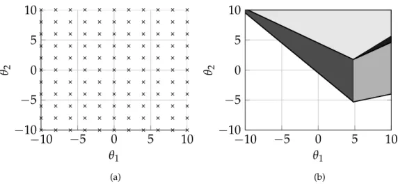
1.1 Two strategies for solving an optimisation problem under uncertainty – (a)

grid optimisation; (b) multi-parametric programming. . . 13

1.2 Principle of optimality (Bellman, 1957) for a generic multi-stage decision process. Figure adapted from (Sieniutycz,2000). . . 15

1.3 Model predictive control - receding horizon scheme. . . 17

1.4 Framework for the development of explicit model predictive controllers. Figure adapted from (Pistikopoulos,2009). . . 19

2.1 Model predictive control as a multi-stage process with Ndecision stages. . . 33

2.2 Map of critical regions for the solution of (2.29) withN=2. . . 39

2.3 Map of critical regions for the solution of (2.29) withN=25. . . 40

2.4 Contour plot showing how the first element of the solution of (2.29) with N=25 is distributed in the parameter space. . . 40

2.5 State-space trajectories for different initial conditions () converging in the set-point (♦). . . 41

2.6 Temporal trajectories of the two components of the system state,x1andx2. . 42

2.7 Temporal trajectory of the control input of the system,u. . . 42

2.8 Comparison of computational times required for the solution of problem (2.29) usingmp-qp, and dynamic programming basedmp-qp. . . 43

3.1 Schematic depiction of process with2stages. . . 49

3.2 Map of critical regions for iterationi =5 of dynamic programming based algorithm with N=6. . . 54

3.3 Comparison of computational times required for the solution of problem (3.17) usingmp-milpand dynamic programming basedmp-milp. . . 54

3.4 Algorithm profile for average between N=4, 5, 6. . . 55

4.1 Map of critical regions for the solution of (4.20) withN=2. . . 70

4.2 Map of critical regions for the solution of (4.20) withN=5. . . 71

4.3 State-space trajectories for different initial conditions () converging to the set-point (♦). . . 71

4.4 Temporal trajectories of the two components of the system state,x1andx2. . 72

4.5 Temporal trajectory of the control input of the system,u. . . 72 4.6 Switching between affine dynamics of (4.20). . . 73 4.7 Comparison of computational times required for the solution of problem

(4.22) usingmp-milpand dynamic programming basedmp-milp. . . 74 5.1 State-space trajectories for different initial conditions () converging to the

set-point (♦) or resulting in infeasible operation (×). . . 84 5.2 Map of critical regions for the solution of (5.33) withN=2. . . 85 5.3 Map of critical regions for the solution of (5.33) withN=5. . . 85 5.4 Map of critical regions for a robust controller with N=2 for different values

ofγ: (a)γ=10%; (b)γ=10%; (c)γ=30%. . . 86 5.5 State-space trajectories for different initial conditions () converging to the

set-point (♦). . . 86

5.6 Temporal trajectories of the two components of the system state,x1andx2. . 87

5.7 Temporal trajectory of the control input of the system,u. . . 87 5.8 Switching between affine dynamics of (5.33). . . 88 6.1 Schematic representation of the distillation column in example6.3.1. . . 96 6.2 Control inputs as a function of the states for the controllers based on the

reduced model with one state. . . 97 6.3 Control inputs as a function of the states for the controllers based on the

reduced model with two states. . . 98 6.4 Critical regions and system trajectory for different disturbances. . . 98 6.5 Closed-loop performance for reduced order onlinenmpcand explicit

multi-parametric controllers (2states). . . 99 6.6 Closed-loop performance for the reduced order controllers with one state

and two states. . . 100 6.7 Closed-loop controller performance for disturbance rejection. . . 100 6.8 Schematic representation of a train ofcstrs. . . 101 6.9 Second component of the control input as a function of the states for reduced

order controller with two states. . . 102 6.10 Critical regions and system trajectory for different disturbances. . . 102 6.11 Output trajectories of the volume in the second reactor for a disturbance of +5%103 6.12 Output trajectories of the temperature in the second reactor for a disturbance

of +5% . . . 104 6.13 Closed-loop controller performance for disturbance rejection. . . 104 6.14 Closed-loop controller performance for disturbance rejection. . . 105

Chapter

1

Introduction

The concept of optimisation has been expressed in a variety of ways, but perhaps the most eloquent and adequate is the following, attributed to Wilde and Beightler (Wilde and Beightler,1967).

Man’s longing for perfection finds expression in the theory of optimisation. It studies how to describe and attain what is Best, once one knows how to measure and alter what is Good or Bad.

While perfection is not always attainable, optimisation provides the mathematical tool that assists in making decisions that minimise undesired outcomes or maximise a certain quality criteria. Mathematically, optimisation corresponds to the problem of finding local or global extreme points of a function, possibly subject to a set of equality or inequality constraints.

Applications of optimisation are numerous and extend to fields of knowledge ranging from production planning, economics, resource allocation, urban planning, engineering, social sciences, and many more. Several textbooks have been devoted to the theory and practice of optimisation techniques (Luenberger,1973; Bertsimas and Tsitsiklis,1997; Schrijver,1998; Winston et al.,2003; Bazaraa et al.,2013).

This thesis is concerned with the concept of multi-parametric programming which, in a way, takes optimisation one step further, by enabling the analysis of the optimal solution of an optimisation problem in face of inexact or unreliable data. The topics explored in this thesis are far from the originally intended purposes of multi-parametric programming, but still maintain the connection to the ideas developed over50 years ago.

This introductory chapter presents a brief overview of the state of the art on multi-parametric programming, with particular emphasis on its applicability in the context of model predictive control. The concept of dynamic programming is also introduced here due to its importance in most of the developments proposed in this thesis. The shortcomings of the state of the art motivate the work on different aspects of the theory of multi-parametric programming which are outlined in the end of the chapter.

Table1.1: Applications of multi-parametric programming.

Application Reference

Energy and environmental analysis (Pistikopoulos et al.,2007a)

Process planning (Hugo and Pistikopoulos,2005), (Li and Ier-apetritou,2007a)

Proactive scheduling (Ryu et al.,2004), (Ryu et al.,2007)

Multi-stage optimisation (Bard, 1983), (Vicente, 2001), (Fa´ısca et al., 2007), (Pistikopoulos et al.,2007a)

Game theory (Fa´ısca et al.,2008)

Model predictive control (Bemporad et al., 2002a), (Pistikopoulos et al.,2007b)

1

.

1

Multi-parametric programming

The first works on parametric programming date as far back as the1950s and are often attributed to Saul Gass and Thomas Saaty (Gass and Saaty,1955).

The idea of moving towards an optimisation strategy that encompasses variations in the objective function or constraints paved the way to many new research directions in optimisation theory. One of the earlier examples of this is attributed to Robinson and Day (Robinson and Day,1974), who used parametric programming to study the effect of round-off errors in the solution of an optimisation problem.

With the establishment of a solid theory on parametric programming, and its exten-sion to the general case of multi-parametric programming, its ideas became important in several fields of study. Table1.1presents a selection of applications in which multi-parametric programming is used.

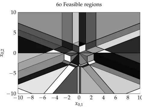
To illustrate the concept of multi-parametric programming, consider the decision faced by a decision maker when solving an optimisation problem with two uncertain parameters,θ1andθ2, with values in the rangeθ∈[−10, 10].

One possible strategy for solving the optimisation problem for the given range of parameters would be to define a grid of points in the space defined byθ1and θ2, as

illustrated in Figure1.1a, and to solve an optimisation problem at each point in the grid. While this approach may be suitable in certain cases, two shortcomings may be identified: a) it is not clear how fine the grid should be in order to capture the most important values of the parameters; b) for the cases in which a fine grid is required, a large number of optimisation problems needs to be solved.

A more elegant solution could be obtained by using multi-parametric programming, with the two uncertain variables,θ1andθ2, being the parameter vector. In contrast to

Figure1.1a, the solution obtained by multi-parametric programming corresponds to a map of regions in the parameter space, denoted critical regions (Figure1.1b), where a certain solution is valid.

In contrast to the grid optimisation approach, the entire parameter space is explored by using multi-parametric programming. Another important piece of information is the region in the parameter space for which no critical region is shown in Figure1.1b,

1.1. Multi-parametric programming 13

−

10

−

5

0

5

10

−

10

−

5

0

5

10

θ

θ

−

10

−

5

0

5

10

−

10

−

5

0

5

10

θ

θ

Figure1.1: Two strategies for solving an optimisation problem under uncertainty – (a) grid optimisation; (b) multi-parametric programming.

which corresponds to combinations of parameters that lead to infeasible solutions of the optimisation problem. The procedure used to solve multi-parametric programming problems and fully explore a given parameter space is described in Chapter2. The results of Figure1.1b may be replicated by solving the example shown in Appendix A. Consider the general formulation of a multi-parametric programming problem given by (1.1). z(θ) =min x,y f(x,y,θ) s.t.g(x,y,θ)≤0 h(x,y,θ) =0 θ∈Θ (1.1)

In problem (1.1),z(θ)is the optimal value of the cost function, f, evaluated at the

optimised set of decision variables which may be continuous, x, or discrete, y. The problem is subject to a set of inequality and equality parametric constraints,gandh, respectively, which may be nonlinear.

The aim of multi-parametric programming is to solve an optimisation problem, such as (1.1) for which the outcome depends on a varying set of parameters,θ, contained in a setΘ, usually pre-defined. The equality constraints often contain the equations defining the discrete-time or continuous-time dynamics of the system under study. The set of inequalities may include physical constraints, production requirements, or any generic constraints imposed on the system.

The solution of problem (1.1) comprises (a) the optimal cost function, z(θ), and the

corresponding optimal decision variables,x∗_(θ)andy∗_{(θ); (b) the map of regions in the}

Table1.2: Review of algorithms for different classes of multi-parametric programming problems.

Problem class References

mp-lp (Gass and Saaty, 1955), (Gal and Nedoma, 1972), (Adler and Monteiro,1992), (Dua and Pistikopoulos,2000), (Borrelli et al., 2003), (Filippi,2004)

mp-qp (Dua et al.,2002), (Bemporad et al.,2002a), (Tøndel et al.,2003b), (Gupta et al.,2011), (Feller et al.,2013)

mp-milp (Acevedo and Pistikopoulos,1997), (Dua and Pistikopoulos,2000), (Li and Ierapetritou,2007b), (Mitsos and Barton,2009), (Wittmann-Hohlbein and Pistikopoulos,2012b)

mp-miqp (Dua et al.,2002)

mp-nlp (Kyparisis, 1987), (Fiacco and Kyparisis, 1988), (Acevedo and Salgueiro,2003), (Bemporad and Filippi,2006), (Grancharova and Johansen,2006), (Dom´ınguez et al.,2010)

mp-minlp (Pertsinidis et al.,1998), (Dua and Pistikopoulos,1999), (Mitsos, 2010)

Depending on properties such as convexity and linearity of the functions f,g, andh, and the presence or not of integer variables, problem (1.1) belongs to a certain class of problems, for which specific algorithms exists.

Table 1.2 presents references to algorithms for solving typical classes of multi-parametric programming problems. The results presented in all chapters of this thesis rely on the existence of algorithms to solve classes of multi-parametric problems pre-sented in Table1.2.

Despite the significant amount of publications and algorithms proposed for the multi-parametric problems presented in Table 1.2, most classes of problems remain active subjects of research. Even for well established classes of problems, such as multi-parametric linear programming problems, there is continued interest in further improving the efficiency of the algorithm, reducing the complexity of exploring large-dimensional parameter spaces, or extending the approach to wider ranges of uncertainty descriptions in the cost function or constraints of the problem.

1

.

2

Dynamic programming

Multi-stage decision processes occur in different fields of study, such as energy planning (Pereira and Pinto,1991; Pistikopoulos and Ierapetritou,1995; Growe-Kuska et al.,2003), computational finance (Pliska,1997; Seydel,2012), computer science (Sakoe,1979; Amini et al.,1990; Leiserson et al.,2001), or optimal control (Bertsekas,1995; Fleming and Soner,2006; Powell,2007).

An illustration of a multi-stage decision process is shown in Figure1.2. The structure of the problem corresponds to a block diagram in which an initial state of the system,s0,

undergoes a sequence ofNdecision stages in which its value is affected by the decision variablesx0,· · ·,xN.

1.2. Dynamic programming 15

Stage

1

Stage

2

. . .

Stage N

s

x

s

x

s

s

s

x

Figure1.2: Principle of optimality (Bellman,1957) for a generic multi-stage decision process. Figure adapted from (Sieniutycz,2000).

Dynamic programming (Bellman,1957; Bertsekas,1995; Sniedovich,2010; Powell, 2007) is an optimisation theory used to efficiently obtain optimal solutions for problems involving multi-stage decision processes by exploring the sequential structure shown in Figure1.2. Dynamic programming has been used to address problems in a variety of fields, such as process scheduling (Bomberger,1966; Choi et al.,2004; Herroelen and Leus,2005), optimal control (Dadebo and McAuley,1995; Bertsekas,1995) or robust control (Nilim and El Ghaoui,2005; Kouramas et al.,2012).

The method is based on the principle of optimality, proposed by Bellman (Bellman, 1957), which states the equivalence of the solution obtained by dynamic programming to the solution obtained using conventional optimisation techniques. The following definition corresponds to the original formulation of the principle of optimality, given by Bellman (Bellman,1957).

Principle of optimality:

An optimal policy has the property that whatever the initial state and initial decision are, the remaining decisions must constitute an optimal policy with regard to the state resulting from the first decision.

The principle of optimality reflects the fact that if a decision taken at stageNof a multi-stage process such as Figure1.2is optimal, it will remain optimal regardless of the decisions taken in previous stages. Having this simple principle in mind, it is possible to transform anN-dimensional problem into a set ofNone-dimensional problems that may be solved sequentially.

The dashed boxes in Figure1.2illustrate this concept. The index irepresents the progression of an algorithm for the solution of the multi-stage problem based on a backwards dynamic programming recursion. For a certain value of i, the optimal decisions of future stages have been determined in previous iterations, and the task is reduced to finding the optimal value ofxN−i. After solving the iterationi=N, the

optimal sequence of decision variables,x0, . . . ,xN−1, is obtained.

Despite the advantages of using dynamic programming in the context of multi-stage decision processes, its use is limited in the presence of hard constraints. In this case, at

each stage of the dynamic programming recursion, linear decisions result and non-convex optimisation procedures are required to solve the dynamic programming problem (Fa´ısca et al.,2008). Another important challenge in constrained dynamic programming is that the computation and storage requirements may significantly increase in the presence of hard constraints (Bertsekas,1995).

To address these issues, different algorithms for constrained dynamic programming have been proposed, combining the principle of optimality of Bellman and multi-parametric programming techniques. By combining these techniques with the principle of optimality, the issues that arise for hard constrained problems are handled in a systematic way, and the shortcomings of conventional dynamic programming techniques are avoided. This method has been used to address constrained dynamic programming problems involving linear/quadratic models (Borrelli et al.,2005; Fa´ısca et al.,2008), and mixed-integer linear/quadratic models (Borrelli et al.,2005).

The use of dynamic programming and multi-parametric programming in the context of explicit model predictive control is described in_§2.3. The concept is extended for the case of constrained dynamic programming of mixed-integer linear problems in Chapter3.

1

.

3

Model predictive control

Model predictive control (Maciejowski and Huzmezan,1997; Mayne et al.,2000; Camacho and Bordons,2004; Rawlings and Mayne,2009) is an advanced control strategy used for the regulation of multi-variable complex plants with strict standards in terms of product specifications and safety requirements. The control problem is formulated as an optimisation problem, which results in optimality of the control inputs with respect to a certain quality criteria, while guaranteeing constraint satisfaction and inherent ability to handle a certain degree of model uncertainty and unknown disturbances (Magni and Sepulchre,1997; Findeisen and Allg¨ower,2002).

The main concept behind model predictive control is illustrated in Figure1.3. The optimisation problem takes place at each time instant,t. The state of the system at timet

is either directly measured or, more commonly, estimated based on the measured output (Lee and Ricker,1994; Mayne et al.,2000). Using this information and the model of the system, the optimiser projects the output of the system over a specified prediction horizon and determines the optimal sequence of inputs that drive the output as close as possible to the desired reference output.

It is possible to operate a model predictive controller in an open-loop fashion, in which the sequence of optimal control inputs determined at timetis only determined once. However, in face of model uncertainty and unknown disturbances, it is more common to apply the scheme in a closed-loop manner: only the first element of the sequence of optimal inputs is applied to the system, and the optimisation procedure is repeated at timet+1. As the optimisation is repeated at timet+1, the prediction

horizon also shifts in time, which is the reason for model predictive control often being referred to as receding horizon control.

1.3. Model predictive control 17

t−2 t−1 t t+1 t+2 t+3 t+4 t+5 t+6 Prediction horizon

Output Current state

Reference output Predicted output Optimal input

Figure1.3: Model predictive control - receding horizon scheme.

Despite the well established benefits of using model predictive control, it has not seen a wide-spread adoption in industrial processes, particularly when the sampling rates of the process are fast. Part of the reason for this is related to the large amounts of legacy controllers based onpid, or other classic controller schemes, and the difficulty in training the plant personnel in the use of a control scheme as drastically different as model predictive control. Another important limitation is related to the computational requirements associated with running an online optimiser at every instance of the sampling time (Engell,2007), despite the recent advances in fast online optimisation (Wang and Boyd,2010).

To address these issues, the idea of explicit model predictive control was developed, combining the principles of model predictive control and multi-parametric programming. These concepts are introduced in_§1.3.1.

1

.

3

.

1

Explicit model predictive control

Explicit model predictive control (Bemporad et al., 2002a; Pistikopoulos et al.,2002, 2007b) is a relatively recent concept, as testified by its absence in important survey papers, such as (Morari and Lee,1999; Mayne et al.,2000). It has, however, been a very significant advance in control theory, and the drive behind much research both in academic topics and applications. A selection of applications reported in the literature, where explicit model predictive control is used, is presented in Table1.3.

The idea behind explicit model predictive control is to link the theory of multi-parametric programming, presented in_§1.1, and model predictive control.

As mentioned in §1.3, a closed-loop model predictive control scheme involves solv-ing an optimisation problem whenever a sample of the system state is available. By formulating the optimisation problem as a multi-parametric programming problem such as (1.1), with the state of the system being the vector of parameters (Bemporad et al.,

Table1.3: Some applications of mp-mpc.

Application References

Active valve train control (Kosmidis et al.,2006)

Cruise control (M¨obus et al.,2003)

Traction control (Borrelli et al.,2006) Direct torque control of induction motors (Papafotiou et al.,2007) Biomedical drug delivery systems (Dua et al., 2006; Krieger

et al.,2013)

Hydrogen storage (Panos et al.,2010)

Marine vessels with rudders (Johansen et al.,2008)

2002a), it is possible to shift the computational effort involved in online optimisation to an offline step in which the optimal solutions for every possible realisation of the state vector are pre-computed.

The use of an explicit model predictive controller as a control device consists therefore of evaluating the state of the system, at every sampling instance, and looking-up the corresponding optimal control input in the pre-computed map of critical regions. This operation is usually significantly faster than repeatedly solving optimisation problems, and therefore the method may be used for systems with more frequent sampling times.

Apart from the reduced computational costs, there is also a benefit in terms of porta-bility. The storage requirements and the processing power required to run an explicit model predictive controller online are relatively low, and the required infrastructure is significantly lower than in the case of conventional model predictive control. This fea-ture motivated the use of the method in applications that require the high performance standard of model predictive control to be achieved in a single chip (Dua et al.,2008).

According to a recent survey paper (Alessio and Bemporad,2009b), the currently available tools for the design of explicit model predictive controllers (ParOS, 2004; Kvasnica et al.,2004) are suitable for applications with sampling times larger than50ms and relatively small size (1-2input variables and5-10parameters). For a study on the hardware implementation of explicit model predictive controllers see (Johansen et al., 2007).

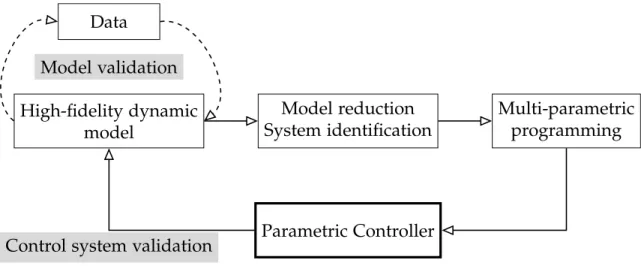
The development of explicit model predictive controllers usually follows the work flow presented by Pistikopoulos (Pistikopoulos,2009). A schematic representation of the framework is presented in Figure1.4.

The need for an intermediate step that reduces the order of the high-fidelity model for which a controller is being designed arises from the limitations of multi-parametric programming algorithms in terms of the size of the problem to be solved, as mentioned above. By using model reduction and system identification techniques, a more tractable problem is defined and currently available software tools may be used to design the controller. To guarantee that this intermediate step does not affect the performance of the controller, closed-loop simulations are performed against the original high-fidelity model, and the entire design procedure repeated, if the results are found to be unsatisfactory.

1.3. Model predictive control 19

High-fidelity dynamic

model

Model reduction

System identification

Multi-parametric

programming

Parametric Controller

Data

Model validation

Control system validation

Figure 1.4: Framework for the development of explicit model predictive controllers. Figure adapted from (Pistikopoulos,2009).

Table1.4: Multi-parametric programming in the context of model predictive control.

Control problem References

Linear discrete systems (Pistikopoulos et al., 2000), (Bemporad et al., 2002a), (Tøndel et al.,2003b)

Linear continuous-time systems (Sakizlis et al.,2005)

Nonlinear systems (Johansen, 2002), (Johansen, 2004), (Sakizlis et al., 2007) (Dom´ınguez et al., 2010), (Rivotti et al.,2012a)

Hybrid systems (Sakizlis et al., 2002), (Borrelli et al., 2005), (Baotic et al.,2006)

Robust control (Bemporad et al., 2003), (Sakizlis et al.,2004), (Pistikopoulos et al.,2009)

extending the theory to several different classes of control problems. Table1.4presents references for problems that are common in the control literature which have been addressed using explicit model predictive control.

1

.

3

.

2

Hybrid explicit model predictive control

Hybrid systems correspond to a class of systems that are described by a combination of continuous variables and logical components. These logical components may result from the presence of discontinuous operating conditions of the equipment, discrete decisions related to availability of components in the system, valves and switches, or the presence of boolean decision rules, such as if-then-else statements.

Hybrid systems find relevance in most processes of practical interest (Pantelides et al.,1999; Branicky et al.,1998). Due to this importance, including integer decision variables in an explicit model predictive control framework has been identified as an

important research direction (Morari and Lee, 1999; Pistikopoulos, 2009). However, the modelling of hybrid systems results in models with integer variables (Raman and Grossmann, 1992; Williams,1999), and therefore in the need to use computationally complex multi-parametric mixed-integer programming algorithms to design the con-trollers. Additionally, as pointed out by Mayne et al. (Mayne et al.,2000), many aspects of conventional model predictive control, such as stability or robustness, require especial treatment in the case of systems involving both continuous and discrete variables.

For this reason, hybrid explicit model predictive control remains an open research topic, and the available theory and algorithms are limited to only a few contributions. The problem of hybrid explicit model predictive control with a linear cost function has been addressed by Bemporad et al. (Bemporad and Morari,1999a) and Baotic et al. (Baotic et al.,2006). Sakizlis et al. (Sakizlis et al.,2002) presented a method based on a mixed-integer quadratic programming algorithm (Dua et al.,2002) that handles quadratic cost functions.

The ability of any algorithm to convert the logical components of the hybrid sys-tem into a suitable formulation relies on the equivalence between propositional logic statements and linear constraints (Cavalier et al.,1990; Raman and Grossmann,1991; Bemporad and Morari,1999a). This property is explored by the mixed logical dynam-ical framework (Bemporad and Morari,1999a) that provides a systematic method of converting logical propositions into a mixed-integer linear formulation.

These ideas are covered in more detail in Chapter4, which presents a novel algo-rithm for hybrid model predictive control based on multi-parametric programming and dynamic programming.

1

.

3

.

3

Explicit robust model predictive control

As discussed in _§1.3, one of the main drawbacks of an open-loop model predictive control implementation is that it assumes the absence of unknown uncertainties and model mismatch. By implementing a closed-loop formulation, in which the optimisation is repeated at each time step, it is possible to reduce the effect of these uncertainties to some extent. This property of model predictive control is referred to as inherent robustness (Mayne et al.,2000).

Despite the inherent robustness of model predictive control, possible model mismatch or external disturbances are not taken into account while optimising the control inputs, which may result in infeasible operation.

Robust model predictive control has the objective of deriving formulations that explicitly take into account uncertainties and guarantee feasible performance for a range of model variations and exterior disturbances.

Several methods for designing robust model predictive controllers have been pro-posed (Campo and Morari, 1987; Zafiriou, 1990; Kothare et al., 1994; Scokaert and Rawlings,1998; Wang and Rawlings,2004). Despite the wealth of publications on the subject, robust model predictive control remains a challenging problem and the existing methods are not at a stage of development suitable for industrial application, except in

1.3. Model predictive control 21 Table1.5: Algorithms for robust multi-parametric programming according to the type of uncertainty description.

Additive Polytopic

References disturbances uncertainty

(Bemporad et al.,2003) x x

(Grancharova and Johansen,2003) x (Kerrigan and Maciejowski,2003) x

(Sakizlis et al.,2004) x

(Alamo et al.,2005) x x

(Manthanwar et al.,2005b) x

(de la Pe ˜na et al.,2005) x x

(de la Pena et al.,2007) x

(Pistikopoulos et al.,2009) x x

(Kouramas et al.,2012) x

very specific cases (Bemporad and Morari,1999b). For a review of the theory and algo-rithms for robust model predictive control see (Bemporad and Morari,1999b; Rawlings and Mayne,2009).

The extension of this methodology to robust explicit model predictive controllers involves further challenges and only recently began to attract the attention of the research community. A selection of publications on this subject is classified in Table1.5according to the type of uncertainty description addressed. These types of uncertainty description are presented in more detail in_§5.1.

Despite these efforts, many issues and areas of robust explicit model predictive control remain to be addressed (Pistikopoulos,2009). One particular aspect in which theory is lacking is the extension of explicit robust control methods to the challenging problem of hybrid explicit model predictive control, for which very few attempts have been published in the literature (Manthanwar et al.,2005b).

Another limitation of conventional robust model predictive control techniques is that the optimisation is performed considering an open-loop control formulation, despite the fact that only the first control input is implemented in the system. The information about past uncertainty values is not taken into account in the optimisation problem, resulting in poor performance of the controller (Lee and Yu,1997). To overcome this limitation, closed-loop formulations based on dynamic programming have been proposed (Lee and Yu,1997; Bemporad et al.,2003).

Chapter5describes a novel algorithm proposed for explicit robust model predic-tive control of hybrid systems with linear cost function, based on multi-parametric programming and dynamic programming.

1

.

3

.

4

Nonlinear explicit model predictive control

The extension of explicit model predictive control to systems described by nonlinear dynamics is of especial importance (Biegler and Rawlings,1991). For these systems, the use of online model predictive control is particularly challenging, since the time required

to compute the solution of the underlying optimisation problem may be significantly larger than the sampling time (Findeisen et al.,2007).

However, the theoretical basis required for applying multi-parametric programming to nonlinear model predictive control is far from being well established (Dom´ınguez et al.,2010). One of the reasons for this is that, as mentioned in_§1.3.1, the aim of explicit model predictive control is to determine the complete map of optimal control actions for every possible realisation of the system state. While this may be achieved for linear systems, in the case of nonlinear systems only an approximation of the map of optimal control inputs may be expected to be obtained. The choice of a general approximate algorithm for such task is not simple, since the type of nonlinearities in the model varies from system to system.

By considering different approximation methods, several algorithms for approxi-mate nonlinear explicit model predictive control have been proposed in the literature (Johansen,2002,2004; Sakizlis et al.,2007; Dom´ınguez et al.,2010). For an overview and comparison of these algorithms see (Dominguez and Pistikopoulos,2011).

An additional challenge in designing nonlinear explicit model predictive controllers is due to the limitations of multi-parametric programming known for systems with high dimensionality (Alessio and Bemporad,2009a), which are especially relevant in the case of nonlinear systems.

In Chapter6, a method is presented that combines model approximation techniques and nonlinear multi-parametric programming algorithms to derive explicit controllers for nonlinear systems. One of the key challenges in this aspect is to select a model approximation methodology that effectively reduces the dimensionality of the model, but keeps track of the main nonlinear dynamics of the system.

1

.

4

Thesis goals and outline

The fundamental concepts of multi-parametric programming for linear and quadratic problems are presented in Chapter2. The chapter begins with the presentation of a general multi-parametric programming problem, for which the optimality conditions are derived. By using local sensitivity analysis results, it is shown how, under certain assumptions, the optimal solution of the general problem may be expressed as a piece-wise affine function of the varying parameters. It is also shown how the solution of model predictive control problems may be obtained by recasting the optimal control formulation as a multi-parametric programming problem where the initial state of the system is the vector of parameters. The chapter concludes with the presentation of a methodology for the solution of explicit model predictive control problems that combines multi-parametric programming and dynamic programming. An illustrative example demonstrates the benefits of using the approach based on multi-parametric programming and dynamic programming, as opposed to conventional methods for explicit model predictive control.

Chapter3addresses the topic of constrained dynamic programming for problems involving multi-stage mixed-integer linear formulations with a linear objective function.

1.4. Thesis goals and outline 23 It is shown that such problems may be decomposed into a series of multi-parametric mixed-integer linear problems, of lower dimensionality, that are sequentially solved to obtain the globally optimal solution of the original problem. At each stage, the dynamic programming recursion is reformulated as a convex multi-parametric programming problem, therefore avoiding the need for global optimisation that usually arises in hard constrained problems. The proposed algorithm is applied to a problem of mixed-integer linear nature that arises in the context of inventory scheduling. The example also highlights how the complexity of the original problem is reduced by using dynamic programming and multi-parametric programming.

Based on the developments of Chapter3, an algorithm for explicit model predictive control of hybrid linear systems is presented in Chapter 4. The proposed method employs multi-parametric and dynamic programming techniques to disassemble the original model predictive control formulation into a set of smaller problems, which can be efficiently solved using suitable multi-parametric mixed integer programming algorithms. The proposed developments are demonstrated with an example of the optimal control of a piece-wise affine system with a linear cost function.

Chapter5builds on the methodology presented in Chapter4and extends it to the problem of explicit robust model predictive control of hybrid systems where uncertainty is present in the model. To immunise the explicit controller against uncertainty, the constraints are reformulated taking into account the worst-case realisation of the uncer-tainty in the model, while the objective function is considered to have its nominal value. It is shown how the reformulation leads to an explicit hybrid model predictive control problem that may be solved using the methods proposed in Chapter4.

Chapter6presents a methodology to derive explicit multi-parametric controllers for nonlinear systems, by combining model approximation techniques and multi-parametric model predictive control. Particular emphasis is given to an approach that applies a nonlinear model reduction technique, based on balancing of empirical gramians, which generates a reduced order model suitable for explicit nonlinear model predictive control algorithms. This approach is compared with a recently proposed method that uses a meta-modelling based model approximation technique which can be directly combined with standard multi-parametric programming algorithms. The methodology is illustrated for two nonlinear models, of a distillation column and a train of cstrs, respectively.

Chapter7presents a summary of the main developments presented in this thesis, and indications of future research directions in the topics of nonlinear explicit model predictive control, robust explicit model predictive control, and constrained dynamic programming of hybrid systems.

The goals of this thesis are summarised as follows.

• Provide a qualitative discussion of the benefits in terms of computational time of a

methodology for the solution of constrained multi-stage optimisation problems by dynamic programming and multi-parametric programming.

• Propose an algorithm for constrained dynamic programming for problems involv-ing multi-stage mixed-integer linear formulations and a linear objective function.

• Demonstrate by means of an illustrative example the computational benefits of using the proposed algorithm for constrained dynamic programming of mixed-integer linear problems.

• Apply the developments proposed for constrained dynamic programming of

hybrid linear problems as the basis for an algorithm for explicit model predictive control of hybrid systems with linear cost function.

• Present an algorithm, based on the proposed developments in constrained dynamic programming and explicit model predictive control, for robust explicit model predictive control of hybrid systems in the case where the model dynamics are affected by worst-case type of uncertainty.

• Develop an algorithm for explicit nonlinear model predictive control by combining multi-parametric programming and model approximation techniques. In this context, compare the use of a nonlinear model reduction technique with a meta-modelling based model approximation technique.

Chapter

2

Multi-parametric programming and explicit model predictive control

This chapter presents fundamental concepts of multi-parametric programming and explicit model predictive control. A general formulation of a multi-parametric problem is shown in§2.1and it is shown how sensitivity analysis results may be used to derive the explicit solution for the particular case of linear or quadratic multi-parametric programming.

In_§2.2, a procedure is presented for reformulating a model predictive control problem with quadratic objective function as a multi-parametric programming problem for which the explicit solution is obtained. Some properties of model predictive control, such as stability and importance of the choice of weights in the objective function, are also discussed in this section.

In §2.3 it is shown how explicit model predictive controllers may be efficiently designed using a combination of multi-parametric programming and dynamic program-ming.

The two approaches used to derive explicit model predictive controllers are compared in §2.4 by using an illustrative example, and conclusions are drawn regarding the computational benefits of using the approach based on dynamic programming.

2

.

1

Fundamentals of multi-parametric linear and quadratic

programming

A general multi-parametric programming problem with a vector of continuous decision variables,x∈Rn_{, and a vector of parameters,(θ∈Θ)∈R}m_{, may be represented in the}

form (2.1). z(θ) =min x f(x,θ) s. t. g(x,θ)≤0 h(x,θ) =0 θ∈Θ (2.1)

In (2.1),z(θ) ∈Ris the optimal value of the cost function, f(x,θ)∈ R, evaluated at the optimal set of continuous decision variablesx ∈Rn_{. The problem is subject to}

a set of inequality and equality parametric constraints, g(x,θ)∈Rp_{andh(x,θ)∈ R}q_,

respectively.

In the remaining of this section, it is shown how the solution of problem (2.1) may be computed, under certain conditions, using principles of sensitivity analysis. The two components that define the solution of (2.1) are:

(a) The explicit expressions of optimal cost function, z∗_{(θ), and the corresponding}

optimal decision variables,x∗_(θ);

(b) The map of regions in the parameter space (critical regions) for which the optimal functions are valid.

The procedure for solving problem (2.1) is based on the principles of local sensitivity analysis and parametric nonlinear programming. The general idea of the procedure is to derive the optimality conditions of (2.1) and analyse how these are affected by perturbations in the parameter vector.

The Lagrangian function of problem (2.1),L(x,θ,λ,µ)is defined as (2.2).

L(x,θ,λ,µ) = f(x,θ) + p

∑

∑

The first order Karush-Kuhn-Tucker optimality conditions (Bazaraa et al., 2013) for problem (2.1) have the form of (2.3).

∇xL(x,θ,λ,µ) =0 λ_ig_i(x,θ) =0 hj(x,θ) =0 λi ≥0 gi(x,θ)≤0 , ∀i=1, . . . ,p ∀j=1, . . . ,q (2.3)

2.1. Fundamentals of multi-parametric linear and quadratic programming 27 The vectorsλiandµjin (2.3) correspond to the Lagrange multipliers of the inequality

and equality constraints, respectively.

Under certain assumptions, the optimality conditions of the general problem (2.1) may be tracked in the neighbourhood of a certain parameter realisation,θ0, providing an

explicit function of the optimizer, x(θ), and the Lagrangian multipliers, λ(θ)andµ(θ),

as a function of the parameters. The existence of this function is ensured by Theorem1. Theorem1. Local Sensitivity Theorem (Fiacco,1976)

Letθ0be a particular parameter realisation of (2.1)andη= [x0,λ0,µ0]T the solution of (2.3).

Under the following assumptions:

Assumption1. Strict complementary slackness (scs) (Tucker,1956). Assumption2. Linear independence constraint qualification (licq). Assumption3. Second order sufficiency condition (sosc).

In the neighbourhood ofθ0, there exist unique and once continuously differentiable functions

x(θ),λ(θ)andµ(θ).

Moreover, the jacobian of system(2.3)is defined by matrices M0and N0, such as:

M0=               ∇2xL ∇xg1 . . . ∇xgp ∇xh1 . . . ∇xhq −λ1∇Txg1 −V1 ... ... 0 −λp∇Txgp −Vp ∇Txh1 ... 0 0 ∇Txhq               (2.4) where Vi =gi(θ0), N0= [∇2θxL,−λ1∇Tθ(∇xg1), . . . ,−λp∇Tθ(∇xgp),∇Tθh1, . . . ,∇θThTq]T (2.5)

The following corollary shows that the explicit parametric expressions mentioned in Theorem1,x(θ),λ(θ)andµ(θ), are piece-wise affine functions of the parameterθ. Corollary1. First-order estimation of x(θ),λ(θ)andµ(θ)in the neighbourhood ofθ0(Fiacco,

1976).

Under the assumptions of Theorem1, the first-order approximation of x(θ),λ(θ)andµ(θ)in the neighbourhood ofθ0is given by:

   x(θ) λ(θ) µ(θ)   =    x(θ0) λ(θ0) µ(θ0)   −M −1 0 N0(θ−θ0) +o(kθk) (2.6)

To determine the optimal expressions ofx(θ),λ(θ), andµ(θ)using (2.6), it is required

to compute the inverse of (2.4). The existence of such inverse is guaranteed by the assumptions of Theorem1(McCormick,1976).

The results guaranteed by Theorem1and Corollary1are important in the sense that they provide means of determining the optimal values of any general problem such as (2.1) as affine expressions of the parameters. However, the need to compute matrices (2.4) and (2.5) may be avoided in the special case of multi-parametric linear or quadratic problems.

A multi-parametric quadratic problem with linear constraints may be written in the form (2.7). Note that a multi-parametric linear problem may be obtained from (2.7) by settingQ=0. z(θ) =min x c T_x+1 2xTQx s. t. Ax≤b+Fθ θ∈Θ (2.7)

In problem (2.7),c∈Rn _{is the cost associated with the linear term,Q∈ R}n×n _{is a}

positive definite matrix defining the cost of the quadratic term, and A∈Rp×n_,b∈Rp_,

and F∈Rp×m_{are linear inequality coefficients.}

For a problem such as (2.7), it is possible to prove that the explicit optimal function is an affine function of the parameters by writing the Karush-Kuhn-Tucker optimality conditions and performing algebraic operations. These results are given by Theorem2. Theorem2. Explicit optimal solution of (2.7)(Dua et al.,2002)

Let Q be a symmetric and positive definite matrix and the assumptions of Theorem1hold. Then the optimal vector, x, and the Lagrange multipliers,λ, are affine expressions of the parameter

vector,θ, in a neighbourhood ofθ0.

Proof. The first order Karush-Kuhn-Tucker conditions of (2.7) are given by:

c+Qx+ATλ=0 (2.8)

λi(Aix−bi−Fiθ) =0, ∀i=1,· · ·,p (2.9)

λi ≥0, ∀i=1,· · ·,p (2.10)

SinceQis a symmetric and positive definite matrix, it is possible to rearrange (2.8) in a form that showsxas an affine function ofλ:

x=−Q−1_(AT_{λ+c) (2.11)}

Let ˜λdenote de Lagrange multipliers corresponding to active inequality constraints. For active constraints the following relation shows thatxis an affine function ofθ:

˜

2.1. Fundamentals of multi-parametric linear and quadratic programming 29 Replacing (2.11) in (2.12) we obtain:

−AQ˜ −1_(AT_{λ˜+c)−b˜−F˜θ=0 (2.13)}

˜

λ=−(AQ˜ −1A˜T)−1F˜θ−(AQ˜ −1A˜T)−1(AQ˜ −1c+b)˜ (2.14)

Equation (2.14) shows the affine relation betweenλandθ. Note that the existence of the term(AQ˜ −1A˜T)−1is guaranteed by the assumption that the rows of ˜Aare linearly

independent and Q is a positive definite matrix.

Remark1. It is possible to obtain a solution for(2.7)in the case when Q is a positive semi-definite matrix. Algorithms that handle this case, referred to as dual degeneracy, are discussed in (Tondel et al.,2003).

As mentioned above, the affine expressions obtained using(2.6), or (2.12) and (2.14), are valid in a neighbourhood ofθ0. To obtain the region in the parameter space (critical

region, CR), where each affine expression is valid, feasibility and optimality conditions are enforced (Dua et al.,2002; Bemporad et al.,2002a) as shown in (2.15).

CR=

θ| g(x(˘ θ),θ)≤0,h(x(θ),θ) =0, ˜λ(θ)≥0, CRI (2.15)

In (2.15), ˘g(x(θ),θ)corresponds to the inactive inequality constraints of (2.1), ˜λ(θ)

are the Lagrange multipliers corresponding to the active inequality constraints and CRI

corresponds to a user-defined initial region in the parameter space that is to be explored. Having defined the critical region in which the affine expressions are valid, a strategy is required to fully explore the pre-defined parameter space, CRI, in order to obtain a

complete map, such as in Figure1.1b.

Dua et al. (Dua et al.,2002) proposed an algorithm that geometrically partitions the parameter space and recursively explores the newly defined partitions until the entire space is explored. This approach is usually preferred to sub-optimal methods (Johansen et al.,2000), or methods that are applicable for problems with constraints only in the decision variables (Seron et al.,2000).

A different approach to exploring the entire parameter space, CRI, has recently been

suggested, motivated by the exponential increase in computational complexity observed for parameter spaces of large dimensionality (Gupta et al.,2011; Feller et al.,2012). The idea behind this method is to enumerate all possible combinations of active constraints of (2.1) and directly compute the explicit solutions using the relations (2.6), or (2.12) and (2.14). This method was shown to be effective for problems with large dimensionality of the parameter space, but small number of constraints.

Regardless of the procedure used to partition the parameter space, the final map of critical regions is identical, given the uniqueness of the optimal piece-wise affine solution, guaranteed by the convexity and continuity of (2.7) (Fiacco and Ishizuka,1990; Dua et al., 2002). To achieve this minimal representation, software solutions for multi-parametric

programming (ParOS,2004; Kvasnica et al.,2004) usually include a post-processing step that merges partitions with the same optimal solution into a convex critical region.

Despite the usefulness of the theory presented in this section, it should be noted that the first order approximation is made due to its practical usefulness, even though a piece-wise affine form is not the natural representation of the solution of (2.7). One possible consequence of this is that the neighbourhoods in which the affine expressions are valid may be narrow, resulting in a large number of critical regions in the final map. For implementation purposes, having a large number of critical regions may imply that the time required to retrieve the optimal solution from the map of critical regions is larger than the sampling time of the system.

To address the issue of point location in highly partitioned maps of critical regions, a method presented in the literature (Tøndel et al.,2003a) proposed the computation of a binary search tree that allows the efficient retrieval of the optimal solution.

2

.

2

Explicit model predictive control

Consider a discrete-time linear system described by the dynamic equations (2.16).

(

xk+1=Axk+Buk

yk=Cxk+Duk (2.16)

The indexkrepresents the temporal coordinate of the state vector,xk ∈Rm, input

vector,uk∈Rn_{, and output vector,yk∈R}my_{. In this section, the coefficientsA∈R}p×m_,

B∈Rp×n_,C∈Rpy×m_{, andD∈R}py×n _{are assumed to be time invariant and unaffected}

by uncertainty. A discussion of explicit model predictive control where the model is unreliable is presented in Chapter5.

A model predictive control problem is an optimisation formulation used to design a controller based on a dynamical model such as (2.16). The problem of regulating (2.16) to the origin, x =0, subject to constraints in the input and state vectors and using a quadratic cost function, is described as (2.17).

U= argmin u0,...,uN−1 kxNk2P+kuN−1k2R+ N−1

∑

In (2.17),kak2Xis the square of the Euclidean norm,(aTXa) 1

2, and Ncorresponds to the output horizon, which for simplicity is assumed to be equal to the control horizon. The strategy to reformulate (2.17) as an explicit model predictive control problem involves re-writing (2.17) as a multi-parametric quadratic problem, such as (2.7), with the parameter vector corresponding to the initial state of system,x0(Pistikopoulos et al.,

2.2. Explicit model predictive control 31 The reformulation of (2.17) as a multi-parametric quadratic problem is given by (2.18). U(θ) =argmin U 1 2UTHU+θTFU s. t. Xmin≤Aˆθ+BUˆ ≤Xmax Umin≤U≤Umax θ=x0 F=2 ˆATQˆBˆ, H=2(BˆTQˆBˆ+R)ˆ ˆ A=          A A2 A3 ... AN          , Bˆ=          B 0·B · · · 0·B AB B · · · 0·B A2B AB B · · · 0·B ... ... ... ... ... AN−1_{B A}N−2_{B · · · AB B}          ˆ Q=       Q 0·Q · · · 0·Q 0·Q Q · · · 0·Q ... ... 0·Q 0·Q 0·Q · · · P       , Rˆ =        0·R 0·R · · · 0·R 0·R 0·R ... ... ... 0·R · · · R        X=hx1 x2 · · · xN iT , U=hu0,u1,· · ·,uN−1 iT (2.18)

Note that the term θTFU in the objective function of (2.18) may be handled in a multi-parametric quadratic programming formulation by introducing the change of variableU = Z−H−1_FT_{θ (Dua et al., 2002), and taking Z as the new optimisation}

variable.

Problem (2.18) is in the form of the multi-parametric quadratic programming formu-lation (2.7) and may be solved using the method presented in_§2.1.

One of the advantages of model predictive control is the ability to handle generic constraints. Additional constraints, specific to the application being considered, may be easily added to the formulation (2.18) without loss of generality.

The reformulation presented in this section may be adapted in a straightforward way to different model predictive control strategies, such as reference output tracking, constraint softening, or to include penalties to the rate of change in the input vector (Bemporad et al.,2002a).

2

.

2

.

1

Closed-loop stability

Stability is the study of the convergence of the state of the system to the origin and is concerned with providing results that guarantee such convergence under certain conditions.

Since the explicit solution of (2.17), obtained using multi-parametric programming, is an exact solution, well established stability results for model predictive control are inherited in the case of explicit model predictive control.

There are different methods of guaranteeing closed-loop stability for constrained receding horizon model predictive control problems.

When the system is open-loop stable, linear, and with convex control constraints, stability may be guaranteed by choosing the terminal weight in (2.17),P, as the solution of the Lyapunov equation (Rawlings and Muske,1993).

Another possibility is to introduce an end-constraint that forces the state to the origin at the end of the control horizon (Kwon and Pearson,1977; Kwon et al.,1983), which guarantees stability in a straightforward way, but may cause infeasible solutions for low values of the control horizon. A more common approach is to define a region, for example the maximal constraint admissible set (Gilbert and Tan,1991), and to replace the terminal equality constraint by an inequality that forces the final state to lie in such region (Michalska and Mayne,1993).

In cases for which it is computationally undesirable to include a terminal constraint, or a terminal set constraint, it is possible to introduce a stabilizing feedback based on the solution of the infinite-horizon quadratic regulator and choose an output horizon large enough to guarantee stability (Chmielewski and Manousiouthakis,1996; Scokaert and Rawlings,1998).

A discussion of different approaches to stability of closed-loop systems may be found in the model predictive control literature survey papers (Garcia et al.,1989; Morari and Lee,1999; Mayne et al.,2000).

2

.

2

.

2

Choice of weights

The choice of matrices Qand Rin (2.17), reflects the relative penalties attributed to deviations in the state of the system and high magnitude of inputs actions, respectively, and is part of the procedure referred to as the tuning of model predictive control. Despite the importance of such procedure, the strategies used for tuning model predictive are often based on heuristics or trial and error, and robust performance is not guaranteed even for the case of unconstrained systems (Rowe and Maciejowski,2000).

For practical purposes, the most common strategy is to tune the control horizon and terminal weight,P, for stability purposes, as discussed in§2.2.1, and leave the task of fine-tuning parametersQandRto the control engineers who are familiar with the production requirements (Dua et al.,2002; Garriga and Soroush,2010).

There have been, nevertheless, some attempts at providing systematic rules for tuning the objective parameters (Rustem et al.,1978; Lee and Ricker,1994; Rustem,1998; Rowe and Maciejowski,1999; Trierweiler and Farina, 2003; Chmielewski and Manthanwar, 2004; Baric et al.,2005).

For an overview of the literature on tuning different model predictive control param-eters, see the recent survey paper (Garriga and Soroush,2010).