DOI: 10.1002/for.2680
R E S E A R C H A R T I C L E
Sparse Bayesian vector autoregressions in huge dimensions
Gregor Kastner
1Florian Huber
21Institute for Statistics and Mathematics,
WU Vienna University of Economics and Business, Vienna, Austria
2Salzburg Centre of European Union
Studies (SCEUS),University of Salzburg, Salzburg, Austria
Correspondence
Gregor Kastner, Institute for Statistics and Mathematics, WU Vienna University of Economics and Business,
Welthandelsplatz 1, 1020 Vienna, Austria. Email: [email protected]
Abstract
We develop a Bayrewriting the error term esian vector autoregressive (VAR) model with multivariate stochastic volatility that is capable of handling vast dimensional information sets. Three features are introduced to permit reliable estimation of the model. First, we assume that the reduced-form errors in the VAR feature a factor stochastic volatility structure, allowing for conditional equation-by-equation estimation. Second, we apply recently developed global–local shrinkage priors to the VAR coefficients to cure the curse of dimensionality. Third, we utilize recent innovations to sample effi-ciently from high-dimensional multivariate Gaussian distributions. This makes simulation-based fully Bayesian inference feasible when the dimensionality is large but the time series length is moderate. We demonstrate the merits of our approach in an extensive simulation study and apply the model to US macroeconomic data to evaluate its forecasting capabilities.
K E Y WO R D S
Dirichlet-Laplace prior, efficient MCMC, factor stochastic volatility, normal-Gamma prior, shrinkage
1
I N T RO D U CT I O N
Previous research has identified two important features that macroeconometric models should possess: the abil-ity to exploit high-dimensional information sets (Ba ´nbura et al., 2010; Koop et al., 2019; Rockova & McAlinn, 2017; Stock & Watson, 2011) and the possibility to cap-ture nonlinear feacap-tures of the underlying time series (Bitto & Frühwirth-Schnatter, 2019; Clark, 2011; Clark & Ravazzolo, 2015; Cogley & Sargent, 2001; Huber et al., 2019; Primiceri, 2005). While the literature suggests sev-eral paths to estimate large models, the majority of such approaches imply that once nonlinearities are taken into account analytical solutions are no longer avail-able and the computational burden becomes prohibitive. This implies that high-dimensional nonlinear models can practically be estimated only under strong (and often unrealistic) restrictions on the dynamics of the model.
However, especially in forecasting applications or in struc-tural analysis, successful models should generally be able to exploit much information and also control for breaks in the autoregressive parameters or, more importantly, changes in the volatility of economic shocks (Koop et al., 2009; Primiceri, 2005; Sims & Zha, 2006).
Two reasons limit the use of large (or even huge) non-linear models. The first reason is statistical. Since the number of parameters in a standard vector autoregression rises quadratically with the number of time series included and commonly used macroeconomic time series are rather short, in-sample overfitting turns out to be a serious issue. As a solution, the Bayesian literature on vector autoregres-sive (VAR) modeling (e.g., Ankargren et al., 2019; Ba ´nbura et al., 2010; Clark, 2011; Clark & Ravazzolo, 2015; Doan et al., 1984; Follett & Yu, 2019; George et al., 2008; Huber & Feldkircher, 2019; Koop, 2013; Korobilis & Pettenuzzo, This is an open access article under the terms of the Creative Commons Attribution License, which permits use, distribution and reproduction in any medium, provided the original work is properly cited.
© 2020 The Authors. Journal of Forecasting published by John Wiley & Sons, Ltd.
2019; Litterman, 1986; Sims & Zha, 1998) suggests shrink-age priors that push the parameter space towards some stylized prior model like a multivariate random walk. On the other hand, Ahelegbey et al. (2016) suggest viewing VARs as graphical models and perform model selection drawing from the literature on sparse directed acyclic graphs. This typically leads to much improved forecast-ing properties and more meanforecast-ingful structural inference. Moreover, the majority of the literature on Bayesian VARs imposes conjugate priors on the autoregressive parame-ters, allowing for analytical posterior solutions and thus avoiding simulation-based techniques such as Markov chain Monte Carlo (MCMC). Frequentist approaches often consider multistep approaches (e.g., Davis et al., 2016).
The second reason is computational. Nonlinear Bayesian models typically have to be estimated by means of MCMC, and computational intensity increases vastly when the number of component series becomes large. This increase stems from the fact that standard algorithms for multivariate regression models call for the inversion of large covariance matrices. Especially for sizable sys-tems, this can quickly turn prohibitive since the inverse of the posterior variance–covariance matrix on the coeffi-cients has to be computed for each sweep of the MCMC algorithm. For natural conjugate models, this step can be vastly simplified because the likelihood possesses a con-venient Kronecker structure, implying that all equations in the VAR feature the same set of explanatory vari-ables. This speeds up computation by large margins but restricts the flexibility of the model. Carriero et al. (2016), for instance, exploit this fact and introduce a simplified stochastic volatility specification. Another strand of the lit-erature augments each equation of the VAR by including the residuals of the preceding equations (Carriero et al., 2019), which also provides significant improvements in terms of computational speed. Finally, in a recent contri-bution, Koop et al. (2019) reduce the dimensionality of the problem at hand by randomly compressing the lagged endogenous variables in the VAR.
All papers mentioned hitherto focus on capturing cross-variable correlation in the conditional mean through the VAR part, and the comovement in volatilities is cap-tured by a rich specification of the error variance (Prim-iceri, 2005) or by a single factor (Carriero et al., 2016). Another strand of the literature, typically used in financial econometrics, utilizes factor models to provide a parsi-monious representation of a covariance matrix, focusing exclusively on the second moment of the predictive den-sity. For instance, Pitt and Shephard (1999) and Aguilar and West (2000) assume that the variance–covariance matrix of a broad panel of time series might be described by a lower dimensional matrix of latent factors featuring
stochastic volatility and a variable-specific idiosyncratic stochastic volatility process.1
The present paper combines the virtues of exploiting large information sets and allowing for movements in the error variance. The overfitting issue mentioned above is solved as follows. First, we use a Dirichlet–Laplace (DL) prior specification (see Bhattacharya et al., 2015) on the VAR coefficients. This prior is a global–local shrinkage prior in the spirit of Polson and Scott (2011) that enables us to heavily shrink the parameter space but at the same time provides enough flexibility to allow for nonzero regression coefficients if necessary. Second, a factor stochastic volatil-ity model on the VAR errors grants a parsimonious rep-resentation of the time-varying error variance–covariance matrix of the VAR. To deal with the computational com-plexity, we exploit the fact that, conditionally on the latent factors and their loadings, equation-by-equation estimation becomes possible within each MCMC itera-tion. Moreover, we apply recent advances for fast sam-pling from high-dimensional multivariate Gaussian distri-butions (Bhattacharya et al., 2016) that permit estimation of models with hundreds of thousands of autoregressive parameters and an error covariance matrix with tens of thousands of nontrivial time-varying elements on a quar-terly US data set in a reasonable amount of time. In a careful analysis, we show to what extent our proposed method improves upon a set of standard algorithms typi-cally used to simulate from the joint posterior distribution of large-dimensional Bayesian VARs.
We first assess the merits of our approach in an exten-sive simulation study based on a range of different data-generating processes (DGPs). Relative to a set of com-peting benchmark specifications we show that, in terms of point estimates, the proposed global–local shrinkage prior yields precise parameter estimates and successfully introduces shrinkage in the modeling framework, without overshrinking significant signals.
In an empirical application, we adopt a modified ver-sion of the quarterly data set proposed by Stock and Wat-son (2011) and McCracken and Ng (2016). To illustrate the out-of-sample performance of our model, we forecast important economic indicators such as output, consumer price inflation, and short-term interest rates, amongst oth-ers. The proposed model is benchmarked against sev-eral alternatives. Our findings suggest that it performs well in terms of one-step-ahead predictive likelihoods. In addition, investigating the time profile of the cumulative log-predictive likelihood reveals that allowing for large information sets in combination with the factor structure especially pays off in times of economic stress.
1Two recent exceptions are Koop and Korobilis (2013) and Carriero et al.
The remainder of this paper is structured as follows. Section 2 introduces the econometric framework. Section 3 details the Bayesian estimation approach, including an elaborated account of the (shrinkage) prior setup adopted and the corresponding conditional posterior distributions. Section 4 provides an analysis of the computational gains of our algorithm relative to a set of established algo-rithms. Section 5 presents the results of an extensive simulation study comparing the performance of carefully selected shrinkage priors for different time series lengths and model dimensions within various (sparse and dense) data-generating scenarios. Section 6, after giving a brief overview of the data set used along with the model spec-ification, illustrates our modeling approach by fitting a single-factor model to 215-dimensional quarterly US data. Moreover, we perform a forecasting exercise to assess the predictive performance of our approach and discuss the choice of the number of latent factors. Finally, Section 7 concludes.
2
ECO N O M ET R I C F R A M E WO R K
Suppose interest centers on modeling anm×1 vector of time series denoted byytwitht=1,…,T. We assume that ytfollows a heteroskedastic VAR(p) process:2yt =A1yt−1+ … +Apyt−p+𝜺t, 𝜺t∼m(0,𝛀t). (1)
Each Aj(j = 1,…,p) is an m × m matrix of
autore-gressive coefficients. The error term is assumed to fol-low a multivariate Gaussian distribution with time-varying variance–covariance matrix𝛀t. To permit reliable and
par-simonious estimation whenmis large, we decompose the residual covariance matrix into
𝛀t =𝚲Vt𝚲+𝚺t, (2)
where both 𝚺t = diag(𝜎12t,…, 𝜎mt2 ) and Vt =
diag(eh1t,…,ehqt)are diagonal matrices with dimension
m and q, respectively, and 𝚲 denotes an m ×q matrix of factor loadings with typical element𝜆ij(i = 1,…,m;
j = 1,…,q). The logarithms of the diagonal elements of
𝚺tandVtfollow AR(1) processes:
h𝑗t =𝜌h𝑗h𝑗,t−1+eh𝑗,t, 𝑗=1,…,q, (3)
log𝜎it2=𝜇𝜎i+𝜌𝜎i(log𝜎i2,t−1−𝜇𝜎i)+e𝜎i,t, i=1,…,m. (4)
To identify the scaling of the elements of𝚲, the process specified in Equation (3) is assumed to have mean zero, while𝜇𝜎jin Equation (4) is the unconditional mean of the
log-elements of𝚺tto be estimated from the data (cf.
Kast-ner et al., 2017). The parameters𝜌hjand𝜌𝜎i are a priori
2For simplicity of exposition we omit the intercept term in the following
discussion (which we nonetheless include in the empirical application).
restricted to the interval(−1,1)and denote the persistence of the latent log variances. The error terms ehj,t ande𝜎i,t
constitute independent zero mean innovations with vari-ances 𝜍2
h𝑗 and𝜍𝜎2i, respectively. This specification implies
that the volatilities are mean reverting and thus bounded in the limit.
This error structure is known as the factor stochastic volatility model (see, e.g., Aguilar & West, 2000; Pitt & Shephard, 1999). It can be equivalently written by intro-ducing q conditionally independent latent factors ft ∼
q(0,Vt)and rewriting the error term in Equation (1) as
𝜺𝑡=𝚲ft+𝛈t, 𝛈t∼m(0,𝚺t). (5)
Note that off-diagonal entries of 𝛀t exclusively stem
from the volatilities of the qfactors, while the diagonal entries of𝛀tare allowed to feature idiosyncratic deviations
driven by the elements of𝚺t. This specification reduces the
number of free elements in𝛀t fromm(m+1)∕2 to mq,
where the latter quantity is typically much smaller than the former. In addition, by conditioning on the latent factors, this representation enables us to derive an efficient Gibbs sampler that allows for conditional equation-by-equation estimation. As will be discussed in more detail in Section 3.2, this constitutes a key feature for computationally feasible Bayesian inference when the dimensionality m becomes large.
The model described by Equations (1) and (2) is related to several alternative specifications commonly used in the literature. For instance, assuming thatVt = Iand𝚺t ≡𝜮
for alltleads to the specification adopted in Stock and Wat-son (2005). Settingq=1 and𝚺t≡𝜮yields a specification
that is similar to the one stipulated in Carriero et al. (2016), with the difference that our model imposes restrictions on the covariances whereas Carriero et al. (2016) estimate a full (but constant) covariance matrix. In addition, our model implies that the stochastic volatility enters𝛀tin an
additive fashion.
Before proceeding to the next subsection it is worth summarizing the key features of the model given by Equations (1)–(5). First, we capture cross-variable move-ments in the conditional mean through the VAR block of the model and assume that comovement in conditional variances is captured by a factor structure. Second, the model introduces stochastic volatility by assuming that a large panel of volatilities may be efficiently summarized through a set of latent heteroskedastic factors. This choice is more flexible than a single-factor model for the volatility, effectively providing a parsimonious representation of𝛀t
that is flexible enough to replicate the dynamic behavior of the variances of a broad set of macroeconomic quantities.
3
I N F E R E N C E I N
L A RG E- D I M E N S I O NA L VA R
M O D E L S
Our approach to estimation and inference is Bayesian. This implies that, after specifying a suitable prior distribution on the model parameters, we can combine this prior with the likelihood implied by the data and the model to obtain the corresponding posterior distribution.
3.1
A global–local shrinkage prior
For prior implementation, it proves to be convenient to define ak×1 vector of predictorsxt= (y′t−1,…,y′t−p)′and
anm×kcoefficient matrixB= (A1,…,Ap)withk=mp
to rewrite the model in Equation (1) more compactly as yt=Bxt+𝜺t.Stacking the rows ofyt,xt, and𝜺tyields
Y =XB′+E, (6)
where Y = (y1,…,yT)′, X = (x1,…,x
T)′, and E = (𝜺1,…,𝜺T)′denote the corresponding full data matrices.
Typically, the matrixBis a sparse matrix with nonzero elements mainly located on the main diagonal of A1. In fact, existing priors in the Minnesota tradition tend to strongly push the system towards the prior model in high dimensions. However, especially in large models, an extremely tight prior onBmight lead to severe over-shrinking, effectively zeroing out coefficients that might be important to explainyt. If the matrixBis characterized by a relatively low number of nonzero regression coefficients, a possible solution is a global–local shrinkage prior (Polson & Scott, 2011).
A recent variant that falls within the class of global–local shrinkage priors is the Dirichlet–Laplace (DL) prior put forward in Bhattacharya et al. (2015). This prior possesses convenient shrinkage properties in the presence of a large degree of sparsity of the parameter vectorb = vec(B). In what follows, we impose the DL prior on each of the K=mkelements ofb, denoted bybj, forj=1,…,K:
b𝑗∼(𝜗𝑗𝜁) ⇔ b𝑗∼(0, 𝜓𝑗𝜗2𝑗𝜁2), 𝜓𝑗∼(1∕2), (7) where denotes the double exponential (Laplace) and
the exponential distribution, 𝜓j is an auxiliary scaling
parameter to achieve conditional normality, and the ele-ments of 𝝑 = (𝜗1,…, 𝜗K)′ are local auxiliary scaling
parameters that are bounded to the(K−1)-dimensional simplex K−1 = {𝝑 ∶ 𝜗
𝑗 ≥ 0,∑n𝑗=1𝜗𝑗 = 1}. A nat-ural prior choice for𝜗j is the (symmetric) Dirichlet
dis-tribution with hyperparameter a: 𝜗𝑗 ∼ (a,…,a). In addition,𝜁 is a global shrinkage parameter that pushes all elements inBtowards zero and exhibits an important role in determining the tail behavior of the marginal prior distribution onbj, obtained after integrating out the 𝜗js.
Thus we follow Bhattacharya et al. (2015) and adopt a fully Bayesian approach by specifying a gamma distributed prior on𝜁 ∼ (Ka,1∕2). It is noteworthy that this prior setup has at least two convenient features that appear to be of prime importance for VAR modeling. First, it exerts a strong degree of shrinkage on all elements ofBbut still provides additional flexibility such that nonzero regres-sion coefficients are permitted. This critical property is a feature which a large class of global–local shrinkage pri-ors share (Griffin & Brown, 2010; Carvalho et al., 2010; Polson & Scott, 2011) and has been recently adopted in a VAR framework by Huber and Feldkircher (2019) and within the general context of state-space models by Bitto and Frühwirth-Schnatter (2019). Second, implementation is simple and requires relatively little additional input from the researcher. In fact, the prior heavily relies on a sin-gle structural hyperparameter that has to be specified with care, namelya.
The hyperparameterainfluences the empirical proper-ties of the proposed shrinkage prior along several impor-tant dimensions. Smaller values ofalead to heavy shrink-age on all elements ofB. To see this, note that lower values of a imply that more prior mass is placed on small val-ues of𝜁 a priori. Similarly, whenais small, the Dirichlet prior places more mass on values of𝜗jclose to zero. Since
lower values of𝜁translate into thicker tails of the marginal prior on bj, the specific choice of a not only influences
the overall degree of shrinkage but also the tail behavior of the prior. Letting p̃ denote the number of predictors, Bhattacharya et al. (2015) show that if a is specified as
̃
p−(1+Δ) for anyΔ > 0 to be small, the DL prior displays
excellent posterior contraction rates, and Pati et al. (2014), discuss the shrinkage properties of the proposed prior within the context of factor models. In our application,
̃
p = K(when considering the total number of predictors) orp̃ =k(when considering the number or predictors per equation).
For the factor loadings we independently use a standard normally distributed prior on each element𝜆i𝑗 ∼ (0,1)
fori = 1,…,mandj = 1,…,q. In the empirical appli-cation (Section 6), we consider in addition the row-wise normal-gamma (NG Griffin & Brown, 2010) shrinkage prior discussed in Kastner (2019); that is𝜆i𝑗|𝜏i2𝑗∼(0, 𝜏i2𝑗),
𝜏2 i𝑗|𝜐 2 i ∼ (a𝜆,a𝜆𝜐 2 i𝑗∕2),𝜆 2 i𝑗 ∼ (c𝜆,d𝜆). Furthermore, we
impose a normally distributed prior on the mean of the log-volatility𝜇𝜎𝑗 ∼ (0,M𝜇)withM𝜇denoting the prior variance, and the commonly employed beta distributed prior on the transformed persistence parameter of the log-volatility 𝜌s𝑗+1
2 ∼ (a0,b0)fors ∈ {h, 𝜎}anda0,b0 ∈ R+ to ensure stationarity. Finally, we use a restricted
gamma prior on the innovation variances in Equations (3) and (4),𝜍2
s𝑗 ∼ (
1 2,
1
to control the tightness of the prior. This choice, motivated in Frühwirth-Schnatter and Wagner (2010), implies that if the data are not informative on the degree of time variation of the log-volatilities then we do not bound𝜍2
s𝑗 artificially away from zero, effectively applying more shrinkage than the standard inverted gamma prior.
3.2
Full conditional posterior
distributions
Conditional on the latent factors and the corresponding loadings, the model in Equation (1) can be cast as a sys-tem ofmunrelated regression models for the elements in zt=yt−𝜦ft, labeledzit, with heteroskedastic errors:
zit=Bi•xt+𝜂it, i=1,…,m. (8)
Here we letBi• denote theith row ofBand𝜂it is theith
element of𝜼t. The corresponding posterior distribution of B′
i•isk-variate Gaussian:
B′i•|• ∼(bi,Qi), (9)
with • indicating that we condition on the remaining parameters and latent quantities of the model. The poste-rior variance and mean are given by
Qi= (X̃ ′ iX̃i+𝚽−i1)−1, (10) bi=Qi(X̃ ′ iz̃i). (11)
The diagonal prior covariance matrix of the coefficients related to theith equation is given by𝜱i, the respective
k×kdiagonal submatrix of𝚽=𝜁×diag(𝜓1𝜗2
1,…, 𝜓K𝜗2K).
Moreover,X̃iis aT×kmatrix with typical rowtgiven by Xt∕𝜎itandz̃iis aT-dimensional vector with thetth element
given byzit∕𝜎it. This normalization renders Equation (8)
conditionally homoskedastic with standard normally dis-tributed white noise errors.
The full conditional posterior distribution of𝜓jis inverse
Gaussian:
𝜓𝑗|• ∼iG(𝜗𝑗𝜁∕|b𝑗|,1), 𝑗=1,…,K. (12) The conditional posterior of the global shrinkage parame-ter𝜁 follows a generalized inverse Gaussian (GIG) distri-bution: 𝜁|• ∼ ( K(a−1),1,2 K ∑ 𝑗=1 |b𝑗|∕𝜗𝑗 ) . (13) To draw from this distribution, we use the efficient algorithm of Hörmann and Leydold (2013). Moreover, we sample the scaling parameters𝜗jby first samplingLj
fromL𝑗|• ∼ (a−1,1,2|b𝑗|), and then setting𝜗𝑗 = L𝑗∕∑Ki=1Li.
The conditional posterior distributions of the factors are Gaussian and thus straightforward to draw from. The fac-tor loadings are sampled using “deep interweaving” (see
Kastner et al., 2017), and the parameters in Equations (3) and (4) along the full histories of the latent log-volatilities are sampled as in Kastner and Frühwirth-Schnatter (2014) using the R-packages factorstochvol (Hosszejni & Kastner, 2019) andstochvol(Kastner, 2016).
Our MCMC algorithm iteratively draws from the con-ditional posterior distributions outlined above and dis-cards the first J draws as burn-in. In terms of compu-tational requirements, the single most intensive step is the simulation from the joint posterior of the autoregres-sive coefficients in B. Because this step is implemented on an equation-by-equation basis, speed improvements relative to the standard approach are already quite sub-stantial. However, note that if k is large (i.e., of the order of several thousands), even the commonly employed equation-by-equation sampling fails to deliver a sufficient amount of draws within a reasonable time window. Con-sequently, we outline an alternative algorithm to draw from a high-dimensional multivariate Gaussian distribu-tion under a Bayesian prior that features a diagonal prior variance–covariance matrix in the upcoming section.
4
CO M P U TAT I O NA L A S P ECT S
The typical approach to sampling from Equation (9) is based on the full system and simultaneously sam-ples from the full conditional posterior of B, imply-ing that the correspondimply-ing posterior distribution is a K-dimensional Gaussian distribution with aK×K dimen-sional variance–covariance matrix. Under a nonconjugate prior, the computational difficulties arise from the need to invert the K × K variance–covariance matrix, which requires operations of orderO(m6p3)under Gaussian elim-ination.If a conjugate prior in combination with a constant (or vastly simplified heteroskedastic; see Carriero et al., 2016) specification of 𝛀t is used, the corresponding
variance–covariance features a Kronecker structure which is computationally cheaper to invert and scales better in large dimensions. Specifically, the manipulations of the corresponding covariance matrix are of orderO(m3+k3
), a significant gain relative to the standard approach. How-ever, this comes at a cost since all equations have to feature the same set of variables, the prior on the VAR coeffi-cients has to be symmetric, and any stochastic volatility specification that preserves conjugacy is necessarily overly simplistic.
By contrast, recent studies emphasize the computational gains that arise from utilizing a framework that is based on equation-by-equation estimation. Carriero et al. (2019) and Koop et al. (2019) augment each equation of the system by either contemporaneous values of the endoge-nous variables of the preceding equations or the
resid-uals from the previous equations. Here, our approach renders the equations of the system conditionally inde-pendent by conditioning on the factors. From a computa-tional perspective, the differences between using a factor model to disentangle the equations and an approach based on augmenting specific equations by quantities that aim to approximate covariance parameters are negligible. If we sample from Equation (9) directly, the computations involved are of order O(mk3) = O(m4p3). This already poses significant improvements relative to full system estimation.
One contribution of the present paper is the application of the algorithm proposed by Bhattacharya et al. (2016) and developed for univariate regression models under a global–local shrinkage prior. This algorithm is applied to each equation in the system and cycles through the follow-ing steps:
1. Sample independently ui ∼ (0k,𝚽i) and 𝛅i ∼
(0T,IT).
2. Useuiand𝛅ito constructvi=X̃iui+𝛅i.
3. Solve(X̃i𝚽iX̃ ′
i+IT)wi= (z̃i−vi)forwi.
4. SetB′i• =ui+𝚽iX̃′iwi.
This algorithm outperforms all competing variants dis-cussed previously in situations where k ≫ T, a situ-ation commonly encountered when dealing with large VAR models. In such cases, steps 1–4 can be carried out using O(pm2T2) floating point operations. In situations where k ≈ T, the computational advantages relative to the standard equation-by-equation algorithm mentioned above are modest or even negative. However, note that the cost is quadratic inmand linear inpand thus scales much better when the number of endogenous variables and/or lags thereof is increased. More information on the empirical performance of our algorithm can be found in Section 6.4.
5
S I M U L AT I O N ST U DY
This section aims at comparing the performance of the DL prior with a range of commonly used alternatives. We investigate sparse, intermediate, and dense DGPs, where T ∈ {50,100,150,200,250} and m ∈ {10,20,50,100}. The probability of an off-diagonal entry to be nonzero is 0.01, 0.1, and 0.8 in each of the respective scenarios. In all scenarios, each intercept entry has a 0.1 probability of being nonzero and all diagonal elements are nonzero with probability 0.8. The nonzero elements are randomly generated from Gaussian distributions roughly tuned to yield stable VARs. More concretely, both the mean 𝜇I and the standard deviation𝜎Iof the intercept are set to
0.01, whereas mean and standard deviation of the
diago-nal (D) and the off-diagonal (O) elements are chosen as follows:
• Dense: 80% off-diagonal density level,𝜇D = 𝜎D = 0.15
and𝜇O =𝜎O=0.01.
• Intermediate: 10% off-diagonal density level,𝜇D=𝜎D=
0.15 and𝜇O=𝜎O=0.1.
• Sparse: 1% off-diagonal density level,𝜇D = 𝜎D = 𝜇O =
𝜎O=0.3.
Concerning the errors, we use a single-factor SV specification. The factor loadings are generated from
(0.001,0.0012)to roughly match the above scaling. The AR(1) processes driving the idiosyncratic log-variances are assumed to have mean𝜇𝜎i = −12 with persistences𝜌𝜎i ranging from 0.85 to 0.98 and innovation standard devi-ations 𝜍𝜎i from 0.3 to 0.1. The process driving the factor
log-variance is assumed to be highly persistent, with𝜌h1= 0.99 and𝜍h1=0.1.
For each of the 60 settings, we simulate 10 data sets. For each of these, we run our MCMC algorithm to obtain 2,000 posterior draws after a burn-in of 1,000. Consequently, the posterior means are compared to the true values and root mean squared errors (RMSEs) are computed. Finally, the median of each of these is reported in Table 1. Alongside the DL prior with weak (aDL=a=1∕2) and strong (aDL= a= 1∕kandaDL =a =1∕K) shrinkage, we also consider the NG prior with a single global shrinkage parameter (see Huber & Feldkircher, 2019, for the exact specification) and a standard conjugate Minnesota prior with a single shrinkage parameter aM, implemented by using dummy
observations. For the NG prior we specify the prior on the global shrinkage parameter to induce heavy shrinkage (by setting both hyperparameters of the gamma prior equal to 0.01) and the prior controlling the excess kurtosisaNGis set equal to 1, corresponding to the Bayesian Lasso (see Park & Casella, 2008), andaNG = 0.1. The latter choice places significant prior mass around zero but at the same time leads to a heavy tailed marginal prior. Finally, we report RMSEs of the ordinary least squares (OLS) estimator (if it exists).
As is to be expected, Table 1 reveals strong to severe overfitting of OLS (corresponding to the posterior mode under a flat prior), which can be mitigated to a cer-tain extent when the Minnesota prior with aM = 0.001
is employed instead. Similarly, the DL prior with weak shrinkage (aDL = 1∕2) displays a tendency to over-fit, in particular when T is small. By contrast, the more aggressive DL and NG shrinkage priors show superior performance. Overall, DL(1∕k) and NG(0.1) exhibit low-est RMSEs, where DL(1∕k) performs best in the sparse scenarios, NG(0.1) performs best in the intermediate set-tings, and no clear winner is to be found in the dense
T m Sparse Intermediate Dense 10 20 50 100 10 20 50 100 10 20 50 100 DL (aDL=1/2) 50 0.079 0.081 0.085 0.088 0.083 0.084 0.086 0.089 0.077 0.082 0.087 0.091 100 0.056 0.056 0.056 0.058 0.060 0.060 0.059 0.061 0.056 0.056 0.058 0.060 150 0.043 0.047 0.045 0.046 0.045 0.050 0.048 0.048 0.044 0.049 0.047 0.049 200 0.040 0.040 0.039 0.038 0.043 0.042 0.042 0.041 0.041 0.040 0.040 0.041 250 0.038 0.034 0.034 0.034 0.039 0.038 0.037 0.036 0.038 0.036 0.036 0.037 DL (aDL=1/k) 50 0.055 0.043 0.037 0.033 0.069 0.053 0.049 0.046 0.057 0.041 0.029 0.026 100 0.042 0.035 0.028 0.025 0.050 0.047 0.044 0.041 0.042 0.033 0.026 0.023 150 0.032 0.032 0.023 0.020 0.042 0.040 0.040 0.038 0.036 0.028 0.023 0.021 200 0.031 0.026 0.020 0.017 0.041 0.038 0.036 0.034 0.032 0.027 0.022 0.020 250 0.030 0.022 0.018 0.015 0.036 0.035 0.033 0.032 0.029 0.025 0.020 0.019 DL (aDL=1/K) 50 0.062 0.043 0.038 0.033 0.072 0.054 0.050 0.047 0.063 0.038 0.028 0.027 100 0.050 0.038 0.028 0.025 0.059 0.049 0.046 0.043 0.047 0.035 0.026 0.024 150 0.044 0.033 0.025 0.021 0.054 0.044 0.041 0.039 0.038 0.033 0.024 0.022 200 0.040 0.031 0.022 0.018 0.051 0.041 0.039 0.036 0.039 0.029 0.022 0.021 250 0.037 0.026 0.019 0.016 0.043 0.039 0.036 0.033 0.039 0.027 0.020 0.020 NG (aNG=1) 50 0.063 0.049 0.044 0.042 0.069 0.053 0.049 0.047 0.060 0.042 0.031 0.027 100 0.051 0.042 0.036 0.033 0.054 0.048 0.042 0.039 0.048 0.037 0.027 0.023 150 0.043 0.037 0.031 0.028 0.046 0.042 0.038 0.036 0.040 0.034 0.026 0.021 200 0.039 0.033 0.028 0.025 0.044 0.039 0.036 0.032 0.038 0.031 0.024 0.020 250 0.037 0.029 0.025 0.023 0.039 0.035 0.032 0.031 0.038 0.029 0.022 0.019 NG (aNG=0.1) 50 0.058 0.043 0.038 0.034 0.066 0.052 0.048 0.045 0.055 0.042 0.029 0.026 100 0.043 0.035 0.028 0.024 0.050 0.045 0.039 0.037 0.044 0.034 0.026 0.022 150 0.035 0.031 0.024 0.020 0.040 0.039 0.034 0.032 0.037 0.031 0.023 0.020 200 0.031 0.026 0.021 0.018 0.038 0.034 0.031 0.028 0.031 0.027 0.022 0.019 250 0.030 0.023 0.018 0.016 0.034 0.030 0.028 0.026 0.031 0.024 0.020 0.018 Minnesota (aM=0.001) 50 0.135 0.137 0.164 0.105 0.134 0.140 0.153 0.102 0.131 0.143 0.165 0.107 100 0.092 0.105 0.112 0.136 0.094 0.104 0.109 0.119 0.094 0.105 0.116 0.129 150 0.079 0.083 0.088 0.102 0.077 0.082 0.086 0.094 0.080 0.084 0.090 0.102 200 0.070 0.071 0.075 0.082 0.069 0.070 0.073 0.077 0.070 0.072 0.077 0.085 250 0.058 0.063 0.065 0.070 0.059 0.063 0.064 0.067 0.060 0.064 0.068 0.071 Minnesota (aM=0.0001) 50 0.067 0.052 0.048 0.046 0.073 0.054 0.049 0.045 0.062 0.037 0.028 0.022 100 0.063 0.050 0.047 0.045 0.069 0.052 0.047 0.044 0.059 0.036 0.028 0.022 150 0.061 0.049 0.045 0.044 0.066 0.049 0.045 0.042 0.056 0.035 0.028 0.021 200 0.061 0.047 0.044 0.043 0.065 0.048 0.044 0.041 0.054 0.034 0.027 0.022 250 0.058 0.046 0.042 0.041 0.059 0.046 0.042 0.040 0.053 0.033 0.027 0.021
OLS (if exists)
50 0.158 0.205 DNE DNE 0.158 0.211 DNE DNE 0.160 0.211 DNE DNE 100 0.106 0.128 0.163 DNE 0.107 0.126 0.157 DNE 0.110 0.128 0.165 DNE 150 0.088 0.099 0.112 0.155 0.087 0.098 0.109 0.155 0.090 0.101 0.115 0.167 200 0.080 0.078 0.087 0.104 0.079 0.078 0.085 0.106 0.080 0.080 0.091 0.114 250 0.065 0.071 0.078 0.092 0.066 0.070 0.077 0.086 0.067 0.071 0.081 0.096
TABLE 1 Median RMSEs stemming from 10 simulations per setting
context. Turning towards NG(1) and DL(1∕K) we tend to observe acceptable but slightly inferior overall perfor-mance. The Minnesota prior with aM = 0.0001 yields
an extreme degree of shrinkage, translating into esti-mates of autoregressive coefficients that are very close to zero, irrespectively of the contribution from the
like-lihood. In that sense, it overshrinks most of the nonzero coefficients. Nevertheless, in scenarios with extremely low signal-to-noise ratios (such as the dense scenario withT= 50 and m = 100), this can be beneficial for the overall performance.
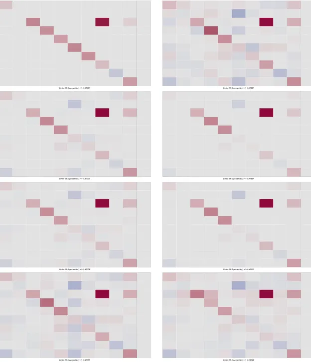
For further illustration, we showcase four exemplary scenarios in Figures A1–A4 in the Appendix.
6
E M P I R I C A L FO R EC A ST I N G
A P P L I C AT I O N
In Section 6.1 we first summarize the data set adopted and present the model specification choices made. Section 6.2 estimates a simple one-factor model to outline the virtues of our proposed framework. Section 6.3 presents the main findings of our forecasting exercise and discusses the choice of the number of factors used for modeling the error covariance structure.
6.1
Data, model specification
and selection issues
The aim of the empirical application is to forecast a set of key US macroeconomic quantities. To this end, we use the quarterly data set provided by McCracken and Ng (2016), a variant of the well-known Stock and Watson (2011) data set for the USA.3 The data span the period ranging from 1959:Q1 to 2015:Q4. We includem = 215 quarterly time series, capturing information on 14 important segments of the economy and follow McCracken and Ng in transform-ing the data to be approximately stationary. Furthermore, we standardize each component series to have zero mean and variance one. In the empirical examples we include p=1 lags of the endogenous variables.4The hyperparam-eters are chosen as follows:M𝜇 = 10,a0 = 20,b0 = 1.5, 𝜉=1,a𝜆=0.1,c𝜆=d𝜆=1.
6.2
Some empirical key features of the
model
To provide some intuition on how our modeling approach works in practice, we first estimate a simple one-factor model (i.e., q = 1) and investigate several features of our empirical model. In the next section we will perform an extensive forecasting exercise and discuss the optimal number of factors in terms of forecasting accuracy.
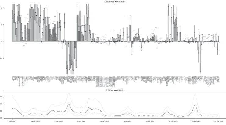
We start by inspecting the posterior distribution of 𝚲 and assess what variables load heavily on the latent factor.
3In addition to quarterly observations, McCracken and Ng (2016) also
provide a subset of the data which is observed monthly. Of course, our method is analogously applicable to higher frequency observations. How-ever, given that the computational cost of the Bhattacharya et al. (2016) approach is quadratic in T, the run-time gains of their approach in comparison to equation-by-equation estimation is then smaller and can, depending on the number of lags, even become be negative.
4We have also experimented with higher lag orders and also found some
evidence of signals at lag two for the data set at hand; see Figures A5–A7 in the Appendix for an illustration. However, out-of-sample predictive studies favored one lag only (cf. Section 6.3).
It is worth emphasizing that most quantities5 associated with real activity (i.e., industrial production and its compo-nents, gross domestic product (GDP) growth, employment measures) load heavily on the factor. Moreover, expecta-tion measures, housing markets, equity prices, and spreads also load heavily on the joint factor.
To assess whether spikes in the volatility associated with the factor coincide with major economic events, the bot-tom panel of Figure 1 depicts the evolution of the posterior distribution of factor volatility over time. A few findings are worth mentioning. First, volatility spikes sharply dur-ing the mid-1970s, a period characterized by the first oil price shock and the bankruptcy of Franklin National Bank in 1974. After declining markedly during the second half of the 1970s, the shift in US monetary policy towards aggres-sively fighting inflation and the second oil price shock again translate into higher macroeconomic uncertainty. Note that from the mid-1980s onward we observe a gen-eral decline in macroeconomic volatility that lasts until the beginning of the 1990s. There we observe a slight increase in volatility possibly caused by the events surrounding the first Gulf War. The remaining years up to the beginning of the 2000s have been relatively unspectacular, with volatil-ity levels being muted most of the time. In 2000/2001, volatility again increases due to the burst of the dot-com bubble and the 9/11 terrorist attacks. Finally, we observe marked spikes in volatility during recessionary episodes like the recent financial crisis in 2008.
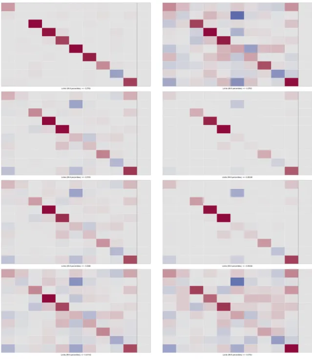
Finally, we assess how well the DL prior witha = 1∕k performs in shrinking the coefficients inBto zero. The top panel of Figure 2 depicts a heat map that gives a rough feel-ing of the size of each regression coefficient based on the posterior median ofB. The bottom panel of Figure 2 depicts the posterior interquartile range, providing some evidence on posterior uncertainty.6 The DL prior apparently suc-ceeds in shrinking the vast majority of the approximately 50,000 coefficients towards zero. Even though not dis-cussed in detail to conserve space, we note that at higher lag orders this very strong shrinkage effect is even more pronounced; see also Figures A5–A7 in the Appendix.
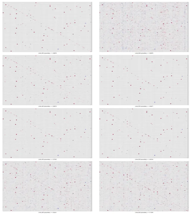
The top panel of Figure 3 displays the posterior median estimates when the shrinkage parameterais chosen to be 1/2 (cf. Bhattacharya et al., 2015, for a discussion of this choice). Whilea=1∕2 appears to provide a fair amount of shrinkage in other applications, for our huge dimensional example this prior exerts only relatively little shrinkage and tends to lead to overfitting. The diagonal pattern in the first lag appears here as well, but there is a considerable
5Hereby we refer to the one-step-ahead forecast error related to a given
time series.
6Since the corresponding posterior distribution is quite heavy tailed,
using posterior standard deviations, while providing a qualitatively sim-ilar picture, tends to be slightly exaggerated.
FIGURE 1 5th, 50th, and 95th posterior percentiles of factor loadings (upper panel) and factor volatility (lower panel) amount of nonzero medians elsewhere. Correspondingly,
the interquartile ranges visualized in the bottom panel of Figure 3 are also very large compared to those obtained witha=1∕k.
Interestingly, for selected time series measuring infla-tion (both consumer and producer price inflainfla-tion) we find that lags of monetary aggregates are allowed to load on the respective inflation series. This result points towards a big advantage of our proposed prior relative to standard VAR priors in the Minnesota tradition: While these priors have been shown to work relatively well in huge dimensions (see Ba ´nbura et al., 2010), they also display a tendency to overshrink when the overall tightness of the prior is inte-grated out in a Bayesian framework, effectively pushing the posterior distribution ofBtowards the prior mean and thus ruling out patterns observed under the DL prior.
Inspection of the interquartile range also indicates that the proposed shrinkage prior succeeds in reducing poste-rior uncertainty markedly. Note that the pattern found for the posterior median ofBcan also be found in terms of the posterior dispersion. We again observe that the coeffi-cients associated with the first, own lag of a given variable are allowed to be nonzero whereas in most other cases the associated posterior is strongly concentrated around zero.
6.3
Predictive evidence
We focus on forecasting gross domestic product (GDPC96), industrial production (INPRO), total nonfarm payroll (PAYEMS), civilian unemployment rate (UNRATE), new
privately owned housing units started (HOUST), con-sumer price index inflation (CPIAUCSL), producer price index for finished goods inflation (PPIFGS), effective fed-eral funds rate (FEDFUNDS), 10-year Treasury constant maturity rate (GS10), US/UK exchange rate (EXUSUKx), and the S&P 500 (SP500). This choice includes the vari-ables investigated by Koop et al. (2019) and some addi-tional important macroeconomic indicators that are com-monly monitored by practitioners, resulting in a total of 11 series.
To assess the forecasting performance of our model, we conduct a pseudo out-of-sample forecasting exercise with initial estimation sample ranging from 1959:Q3 to 1990:Q2. Based on this estimation period, we compute one-quarter-ahead predictive densities for the first period in the hold-out (i.e., 1990:Q3). After obtaining the cor-responding predictive densities and evaluating the corre-sponding log-predictive likelihoods, we expand the estima-tion period and reestimate the model. This procedure is repeated 100 times until the final point of the full sample is reached. The quarterly scores obtained this way are then accumulated.
Our model withq∈ {0,1,…,4}factors is benchmarked against the prior model, a pure factor stochastic volatil-ity (FSV) model with conditional mean equal to zero (i.e., B=0m×k). In what follows we label this specification FSV
FIGURE 2 Posterior medians (top) and posterior interquartile ranges (bottom) of VAR coefficients,a=1∕k=1∕216 [Colour figure can be viewed at wileyonlinelibrary.com]
FIGURE 3 Posterior medians (top) and posterior interquartile ranges (bottom) of VAR coefficients,a=1∕2 [Colour figure can be viewed at wileyonlinelibrary.com]
0. To assess the merits of the proposed shrinkage prior vis-à-vis a Minnesota prior and an NG shrinkage prior we also include the models described in Section 5. Moreover, we include two models that impose the restriction that A1 = Im and A1 = 0.8 ×Im, while Aj for j > 1 are
set equal to zero matrices in both cases. The first model, labeled FSV 1, assumes that the conditional mean ofyt fol-lows a random walk process, and the second specification, denoted by FSV 0.8, imposes the restriction that the vari-ables inytfeature a rather strong degree of persistence but are stationary. The exercise serves to evaluate whether it pays to impose a VAR structure on the first moment of the joint density of our data and to assess how many factors are needed to obtain precise multivariate density predictions for our 11 variables of interest.
Overall log-predictive scores (LPSs) are summarized in Table 2. An immediate finding is that ignoring the error covariance structure (using zero factors) produces rather inaccurate forecasts for all models considered. While a sin-gle factor model improves predictive accuracy by a large margin, allowing for more factors (i.e., even more flexi-ble modeling of the covariance structure) further increases the forecasting performance. For this specific exercise, we identify two or three factors to be a reasonable choice for most models when the joint log-predictive scores of the aforementioned variables are considered. We would like
to stress that this choice critically depends on the number of variables we include in our prediction set. If we focus attention on the marginal predictive densities (i.e., the uni-variate predictive densities obtained after integrating out the remaining elements inyt), we find that fewer or even
no factors receive more support (see Table 3), whereas in the case of higher dimensional prediction sets more than two factors lead to more accurate density predictions (cf. Kastner et al., 2017, for an investigation of this issue in the context of a standard FSV model). As a general remark, we note that identifying the optimal number of factors in high-dimensional FSV models is a challenging problem in practice. Using the deviance information criterion (DIC; cf. Chan & Grant, 2016) may be an option but is likely to be unstable in very high dimensions. The approach adopted in the paper at hand, namely the decomposition of the marginal likelihood into predictive likelihoods (cf. Geweke & Amisano, 2010) tends to be more stable, in par-ticular when interest is placed on predicting subsets only. Moreover, it can be trivially parallelized, thus becoming computationally feasible on high-performance computing infrastructures.
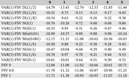
Considering forecasting accuracy across models reveals that our proposed VAR(1)-FSV with a DL(1∕k) prior dis-plays excellent forecasting capabilities, outperforming all competitors. Among the VAR(1) models, DL(1∕K) and TABLE 2 Average log-predictive scores for the
number of factorsq∈ {0,1,…,5}in various VAR-FSV specifications as well as pure FSV models
0 1 2 3 4 5 VAR(1)-FSV DL(1∕2) -14.79 -13.45 -12.74 -12.53 -11.85 -11.44 VAR(1)-FSV DL(1∕k) -10.51 -9.75 -9.15 -9.15 -9.17 -9.43 VAR(1)-FSV DL(1∕K) -10.54 -9.63 -9.22 -9.26 -9.22 -9.38 VAR(1)-FSV NG(1) -10.76 -10.26 -9.72 -9.60 -9.68 -9.86 VAR(1)-FSV NG(0.1) -10.55 -9.95 -9.31 -9.26 -9.47 -9.46 VAR(1)-FSV Min(0.01) -10.99 -10.37 -9.89 -9.88 -9.98 -10.24 VAR(1)-FSV Min(0.001) -12.15 -11.21 -11.08 -10.62 -10.56 -10.83 VAR(2)-FSV DL(1∕k) -10.50 -9.88 -9.22 -9.38 -9.28 -9.43 VAR(2)-FSV NG(0.1) -10.47 -10.04 -9.44 -9.29 -9.40 -9.49 VAR(5)-FSV DL(1∕k) -10.70 -9.97 -9.78 -9.21 -9.44 -9.53 VAR(5)-FSV NG(0.1) -10.61 -10.01 -9.64 -9.51 -9.50 -9.52 FSV 0 -12.08 -11.08 -11.02 -10.66 -10.61 -10.71 FSV 0.8 -11.78 -11.32 -11.06 -10.87 -10.96 -11.25 FSV 1 -11.71 -11.28 -10.95 -10.95 -11.07 -11.18 Note.Estimation and prediction are conducted on allm=215component series; the predic-tive density is then evaluated on the set of 11 variables of interest. Larger numbers indicate better joint predictive density performance.
TABLE 3 Average univariate log-predictive scores for inflation (CPIAUCSL), short-term interest rates (FEDFUNDS), and output growth (GDPC96) withq∈ {0,1,2}factors CPIAUCSL FEDFUNDS GDPC96 0 1 2 0 1 2 0 1 2 VAR(1)-FSV DL(1∕k) -1.03 -1.11 -1.13 -1.26 -1.26 -1.24 0.08 0.05 0.03 VAR(1)-FSV NG(0.1) -1.00 -1.07 -1.10 -1.28 -1.26 -1.22 -0.10 -0.12 -0.15 VAR(2)-FSV DL(1∕k) -1.02 -1.12 -1.14 -1.25 -1.27 -1.22 0.04 -0.01 -0.01 VAR(2)-FSV NG(0.1) -1.00 -1.11 -1.12 -1.26 -1.23 -1.25 -0.14 -0.16 -0.14 VAR(5)-FSV DL(1∕k) -1.05 -1.16 -1.16 -1.29 -1.26 -1.26 -0.02 -0.10 -0.13 VAR(5)-FSV NG(0.1) -1.00 -1.09 -1.13 -1.29 -1.27 -1.25 -0.19 -0.18 -0.21
NG(0.1) also do well, and the Bayesian Lasso (NG(1)) as well as the Minnesota prior with medium shrinkage (Min(0.01)) show decent performance. Clearly, DL(1/2) overfits and Min(0.001) overshrinks. Note that higher lag orders seem rarely to increase predictive accuracy. How-ever, comparing the differences between the benchmark pure FSV models and the VAR-FSV models considered, we find that explicitly modeling the conditional mean improves the forecasting accuracy in practically all cases.
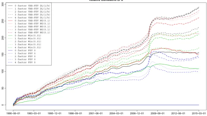
To investigate whether forecasting performance is homogeneous over time, Figure 4 visualizes the cumula-tive LPSs relacumula-tive to the zero-factor FSV model over time. The benefit of the flexible SV structure in the VAR resid-uals is particularly pronounced during the 2008 financial crisis which can be seen by comparing the solid lines to the broken lines. During this period, time-varying covari-ance modeling appears to be of great importcovari-ance and the performance of models that ignore contemporaneous dependence deteriorates. This finding is in line with Kast-ner (2019), who reports analogous results for US asset returns. The increase in predictive accuracy can be traced back to the fact that within an economic downturn the correlation structure of our data set changes markedly, with most indicators that measure real activity sharply declining in lockstep. A model that takes contemporane-ous cross-variable linkages sericontemporane-ously is thus able to fully exploit such behavior, which in turn improves predictions.
Up to this point, we have focused exclusively on the joint performance of our model for the specific set of variables considered. To gain a deeper understanding on how our model performs for relevant selected quantities, Table 3 displays marginal LPSs for the two most promising prior specifications with one, two, and five lags. The variables we consider are inflation (CPIAUCSL), short-term interest rates (FEDFUNDS), and output growth (GDPC96).
In contrast to the findings based on joint LPSs, we observe that models without a factor structure tend to perform better than models that setq>0, with the excep-tion of interest rates where all models predict more or less equally badly. This finding corroborates our conjecture stated above, implying that if the set of focus variables is subsequently enlarged, more factors are necessary in order to obtain precise density predictions. Here, we only focus on marginal model performance, implying that for each variable, contemporaneous relations between the ele-ments inytare integrated out. This, in turn, implies that the additional gain in model flexibility is offset by the com-paratively larger number of parameters. Concerning the difference between VAR priors, it appears that NG slightly outperforms DL for inflation, whereas DL is superior when it comes to predicting output growth.
6.4
A note on the computational burden
Even though the efficient sampling schemes outlined in this paper help to overcome absolutely prohibitivecom-FIGURE 4 Cumulative log predictive scores, relative to a zero-mean model with independent stochastic volatility components for all component series. Higher values correspond to better one-quarter-ahead density predictions up to the corresponding point in time [Colour figure can be viewed at wileyonlinelibrary.com]
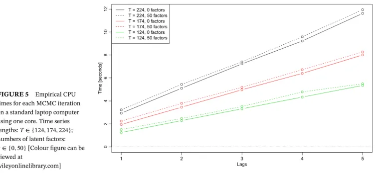
FIGURE 5 Empirical CPU times for each MCMC iteration on a standard laptop computer using one core. Time series lengths:T∈ {124,174,224}; numbers of latent factors:
q∈ {0,50}[Colour figure can be viewed at
wileyonlinelibrary.com]
putational burdens, the CPU time needed to perform fully Bayesian inference in a model of this size can still be con-sidered substantial. In what follows we shed light on the estimation time required and how it is related to the length of the time seriesT, the lag lengthp, and the number of latent factorsq∈ {0,50}. Figure 5 shows the time needed to perform a single draw from the joint posterior distribu-tion of the 215+2152pcoefficients and their corresponding 2(215+2152p)+1 auxiliary shrinkage quantities, theqT fac-tor realizations and the associated 215qloadings, alongside (T+1)(215+q)latent volatilities with their correspond-ing 645+2qparameters. This amounts to 166,841 random draws for the smallest model considered (one lag, no fac-tors,T = 124) and 776,341 random draws for the largest model (5 lags, 50 factors,T=224) at each MCMC iteration. As mentioned above, the computation time rises approx-imately linearly with the number of lags included. Dot-ted lines indicate the time in seconds needed to perform a single draw from a model with 50 factors included, while solid lines refer to the time needed to estimate a model without factors and a diagonal time-varying variance–covariance matrix 𝛀t. Interestingly, the
addi-tional complexity when moving from a model without factors to a highly parametrized model with 50 factors appears to be negligible, increasing the time needed by a fraction of a second on average. The important role of the length of the sample can be seen by comparing the green, red, and black lines. The time necessary to perform a simple MCMC draw quickly rises with the length of our sample, consistent with the statements made in Section 4. This feature of our algorithm, however, is convenient espe-cially when researchers are interested in combining many short time series or performing recursive forecasting based on a tiny initial estimation sample.
7
C LO S I N G R E M A R K S
In this paper we propose an alternative route to estimate huge-dimensional VAR models that allow for time varia-tion in the error variances. The Dirichlet–Laplace prior, a recent variant of a global–local shrinkage prior, enables us to heavily shrink the parameter space towards the prior model while providing enough flexibility that individual regression coefficients are allowed to be unrestricted. This prior setup alleviates overfitting issues generally associ-ated with large VAR models. To cope with computational issues we assume that the one-step-ahead forecast errors of the VAR feature a factor stochastic volatility structure that enables us to perform equation-by-equation estimation, conditional on the loadings and the factors. Since poste-rior simulation of each equation's autoregressive parame-ters involves manipulating large matrices, we implement an alternative recent algorithm that improves upon exist-ing methods by large margins, renderexist-ing a fully fledged Bayesian estimation of truly huge systems possible.
In an empirical application we first present various key features of our approach based on a single-factor model. This single factor, which summarizes the joint dynamics of the VAR errors, can be interpreted as an uncertainty measure that closely tracks observed factors such as the volatility index. The question whether such a simplistic structure proves to be an adequate representation of the time-varying covariance matrix naturally arises, and we therefore provide a detailed forecasting exercise to evalu-ate the merits of our approach relative to the prior model and a set of competing models with a different number of latent factors in the errors.
Finally, three potential extensions are worth mention-ing. First, given the fact that systematic and in-depth
empirical comparisons of the various recently devel-oped roads towards handling high-dimensional VARs with time-varying contemporaneous covariance in a Bayesian framework (VAR-FSV, VAR-Cholesky-SV, com-pressed VAR-SV, etc.) are still missing and it is not clear whether one of these models turns out to dominate the others for all points in time, one could consider averag-ing/selecting dynamically. Second, note that it is trivial to relax the assumption of symmetry for the DL components. In the context of VARs, this might be of particular inter-est for distinguishing diagonal (aDlarge) from off-diagonal
(aO small) elements in the spirit of the Minnesota prior
or increasing the amount of shrinkage with increasing lag order (cf. Huber & Feldkircher, 2019, for a similar setup in the context of the normal-gamma shrinkage prior). Third, we would like to stress that our approach could also be used to estimate huge-dimensional time-varying param-eter VAR models with stochastic volatility. To cope with the computational difficulties associated with the vast state space, a possible approach could be to rely on an addi-tional layer of hierarchy that imposes a (dynamic) factor structure on the time-varying autoregressive coefficients in the spirit of Eisenstat et al. (2018) and thus reduce the computational burden considerably.
AC K N OW L E D G M E N T S
The authors acknowledge funding from the Austrian Sci-ence Fund (FWF) for the project “High-dimensional sta-tistical learning: New methods to advance economic and sustainability policies” (ZK 35), jointly carried out by WU Vienna University of Economics and Business, Paris Lodron University Salzburg, TU Wien, and the Austrian Institute of Economic Research (WIFO).
DATA AVA I L A B I L I T Y STAT E M E N T
The data analyzed in this manuscript are available from the corresponding author on request.
R E F E R E N C E S
Aguilar, O., & West, M. (2000). Bayesian dynamic factor models and portfolio allocation.Journal of Business and Economic Statistics,
18(3), 338–357. https://doi.org/10.2307/1392266
Ahelegbey, D. F., Billio, M., & Casarin, R. (2016). Sparse graph-ical vector autoregression: A Bayesian approach. Annals of
Economics and Statistics, 123–124, 333–361. https://doi.org/10.
15609/annaeconstat2009.123-124.0333
Ankargren, S., Unosson, M., & Yang, Y. (2019). A flexible mixed-frequency vector autoregression with a steady-state prior. arXiv: 1911.09151 [econ.EM].
Ba ´nbura, M., Giannone, D., & Reichlin, L. (2010). Large Bayesian vector autoregressions.Journal of Applied Econometrics,25(1), 71–92. https://doi.org/10.1002/jae.1137
Bhattacharya, A., Chakraborty, A., & Mallick, B. K. (2016). Fast sam-pling with Gaussian scale mixture priors in high-dimensional regression.Biometrika,103(4), 985–991. https://doi.org/10.1093/ biomet/asw042
Bhattacharya, A., Pati, D., Pillai, N. S., & Dunson, D. B. (2015). Dirichlet–Laplace priors for optimal shrinkage.Journal of the
American Statistical Association, 110(512), 1479–1490. https://
doi.org/10.1080/01621459.2014.960967
Bitto, A., & Frühwirth-Schnatter, S. (2019). Achieving shrinkage in a time-varying parameter model framework.Journal of
Econo-metrics, 210(1), 75–97. https://doi.org/10.1016/j.jeconom.2018.
11.006
Carriero, A., Clark, T. E., & Marcellino, M. (2016). Common drifting volatility in large Bayesian VARs.Journal of Business
and Economic Statistics,34(3), 375–390. https://doi.org/10.1080/
07350015.2015.1040116
Carriero, A., Clark, T. E., & Marcellino, M. (2019). Large Bayesian vector autoregressions with stochastic volatility and non-conjugate priors.Journal of Econometrics,212(1), 137–154. https://doi.org/10.1016/j.jeconom.2019.04.024
Carvalho, C. M., Polson, N. G., & Scott, J. G. (2010). The horseshoe estimator for sparse signals.Biometrika,97(2), 465–480. https:// doi.org/10.1093/biomet/asq017
Chan, J. C. C., & Grant, A. L. (2016). Fast computation of the deviance information criterion for latent variable models.Computational
Statistics and Data Analysis, 100, 847–859. https://doi.org/10.
1016/j.csda.2014.07.018
Clark, T. E. (2011). Real-time density forecasts from Bayesian vector autoregressions with stochastic volatility.Journal of Business and
Economic Statistics,29(3), 327–341. https://doi.org/10.1198/jbes.
2010.09248
Clark, T. E., & Ravazzolo, F. (2015). Macroeconomic forecasting per-formance under alternative specifications of time-varying
volatil-ity.Journal of Applied Econometrics,30(4), 551–575. https://doi.
org/10.1002/jae.2379
Cogley, T., & Sargent, T. J. (2001). Evolving post-World War II US inflation dynamics,NBER macroeconomics annual(pp. 331–373), Vol.16. Cambridge, MA: National Bureau of Economic Research. Davis, R. A., Zang, P., & Zheng, T. (2016). Sparse vector autoregres-sive modeling.Journal of Computational and Graphical Statis-tics, 25(4), 1077–1096. https://doi.org/10.1080/10618600.2015. 1092978
Doan, T., Litterman, R. B., & Sims, C. A. (1984). Forecast-ing and conditional projection usForecast-ing realistic prior distribu-tions.Econometric Reviews,3(1), 1–100. https://doi.org/10.1080/ 07474938408800053
Eisenstat, E., Chan, J. C. C., & Strachan, R. W. (2018). Reducing dimensions in a large TVP-VAR. (Working Paper 18-37). Waterloo ON, Canada: Rimini Centre for Economic Analysis.
Follett, L., & Yu, C. (2019). Achieving parsimony in Bayesian vec-tor auvec-toregressions with the horseshoe prior.Econometrics and
Statistics, 11, 130–144. https://doi.org/10.1016/j.ecosta.2018.12.
004
Frühwirth-Schnatter, S., & Wagner, H. (2010). Stochastic model spec-ification search for Gaussian and partial non-Gaussian state space models.Journal of Econometrics,154(1), 85–100. https:// doi.org/10.1016/j.jeconom.2009.07.003
George, E. I., Sun, D., & Ni, S. (2008). Bayesian stochastic search for VAR model restrictions.Journal of Econometrics,142(1), 553–580. https://doi.org/10.1016/j.jeconom.2007.08.017

![FIGURE 2 Posterior medians (top) and posterior interquartile ranges (bottom) of VAR coefficients, a = 1∕k = 1∕216 [Colour figure can be viewed at wileyonlinelibrary.com]](https://thumb-us.123doks.com/thumbv2/123dok_us/646868.2577973/10.892.83.812.65.1027/figure-posterior-medians-posterior-interquartile-coefficients-colour-wileyonlinelibrary.webp)
![FIGURE 3 Posterior medians (top) and posterior interquartile ranges (bottom) of VAR coefficients, a = 1∕2 [Colour figure can be viewed at wileyonlinelibrary.com]](https://thumb-us.123doks.com/thumbv2/123dok_us/646868.2577973/11.892.74.820.70.1052/figure-posterior-medians-posterior-interquartile-coefficients-colour-wileyonlinelibrary.webp)