Department of Economics
Working Paper No. 179
Density Forecasting using Bayesian
Global Vector Autoregressions with
Common Stochastic Volatility
Florian Huber
Density Forecasting using Bayesian Global Vector
Autoregressions with Common Stochastic Volatility
Florian Huber
∗Vienna University of Economics and Business (WU)
Abstract
This paper puts forward a Bayesian Global Vector Autoregressive Model with Common Stochastic Volatility (B-GVAR-CSV). We assume that country specific volatility is driven by a single latent stochastic process, which simplifies the analysis and implies significant computational gains. Apart from computational advantages, this is also justified on the ground that the volatility of most macroeconomic quantities considered in our application tends to follow a similar pattern. Furthermore, Minnesota priors are used to introduce shrinkage to cure the curse of dimensionality. Finally, this model is then used to produce predictive densities for a set of macroeconomic aggregates. The dataset employed consists of quarterly data spanning from 1995:Q1 to 2012:Q4 and includes 45 economies plus the Euro Area. Our results indicate that stochastic volatility specifications influences accuracy along two dimensions: First, it helps to increase the overall predictive fit of our model. This result can be seen for some variables under scrutiny, most notably for real GDP and short-term interest rates. Second, it helps to make the model more resilient with respect to outliers and economic crises. This implies that when evaluated over time, the log predictive scores tend to show significantly less variation as compared to homoscedastic models.
Keywords: Density Forecasting, Stochastic Volatility, Global vector autore-gressions.
JEL Codes: C32, F44, E32, E47.
∗I would like to thank Sylvia Frühwirth-Schnatter, Gregor Kastner, Martin Feldkircher, Jesús Crespo
Cuaresma, participants of the eigth ECB workshop on forecasting techniques and internal research seminars at the Vienna University of Economics and Business. Email: [email protected].
1
Introduction
Recent episodes of rising volatility of several key macroeconomic quantities revealed that most models employed in policy institutions failed to deliver reliable forecasts under such circum-stances. This stems from the fact that practitioners remained largely confined to simple linear models which do not account for structural changes in the behavior of the underlying vari-ables. Two reasons are worth mentioning why the majority of applied researcher still stick to linear models. First, estimation is easy and numerical optimization is often unnecessary. As a consequence, they are easy to implement using standard statistical software packages. Second, linear models are easy to interpret and understand, which makes them valuable for the major-ity of practitioners. However, the recent global turmoil has proved that more flexible models are needed to fully capture the complex dynamics arising in macroeconomics and finance. Es-pecially for highly volatile financial time series non-linear models are needed to fully capture sudden shifts in volatility commonly observed in financial markets.
Several studies provided evidence for a sudden increase of volatility in industrialized economies after experiencing decades of relatively stable and low volatility of macroeconomic fundamen-tals. Linear models, like vector autoregressive models (VARs), which have been performing quite well up to the mid 2000s suddenly failed to produce reliable predictions. Ignoring the dynamic behaviour of volatility led to predictive densities which are either too narrow or too wide, resulting in inflated confidence bounds and poorly estimated probabilities for tail events. Thus it might be necessary to account for heteroscedasticy by means of more flexible specifica-tions of the variance covariance matrix. A plethora of studies emphasized the usefulness of such stochastic volatility specifications in terms of point- and density forecasts. Giordani & Villani
(2010), Clark (2011) and Carrieroet al.(2012) all highlight the substantial increases in
forecast-ing accuracy by usforecast-ing SV specifications. Such gains in accuracy typically directly translate into better prediction intervals produced in central banks and other policy institutions, underlining the practical relevance of this approach.
Despite the fact that stochastic volatility VARs introduce additional flexiblity when it comes to macroeconomic modelling, computational needs also increase substantially. Additionally, due to the fact that frequentist estimated VARs typically suffer from parameter proliferation, which translates into the well-known curse of dimensionality, parameters are imprecisely estimated and such models tend to overfit the data dramatically. Thus, Bayesian methods are needed to obtain reliable estimates and impose shrinkage on the parameters. Furthermore, allowing for flexible stochastic volatility specifications in VARs typically leads to non-conjugate situations where forward-filtering-backward-sampling methods (FFBS) are required. This bounds the analysis usually to small- to medium scale models. Especially in forecasting applications, it is of interest to allow for high dimensional models to exploit information originating from other variables or other countries. Several recent contributions aimed for making the estimation of large scale models feasible and still preserve the flexibility of non-linear models. Koop & Korobilis (2013) draw on ideas from the dynamic model averaging literature and utilize forgetting factors to
reduce the computational burden. In another contribution, Carriero et al. (2012) allow for a
simplified version of stochastic volatility, where it is assumed that the volatility of the whole system is driven by a single, latent process. This assumption preserves the conjugacy of the prior and permits a convenient Kronecker structure of the likelihood. This implies significant computational gains using such a simplified prior structure.
In terms of achieving shrinkage in large scale macroeconometric models, the global vector
way of reducing the dimensionality of the estimation problem. Several contributions outlined the
usefulness of such large scale models to perform forecasting (Pesaran et al., 2009;
Greenwood-Nimmoet al., 2012; Crespo Cuaresma et al., 2014) or impulse response analysis (Pesaranet al.,
2007; Dees et al., 2007). One disadvantage is, however, that frequentist estimation of GVAR
models does not cure the curse of dimensionality at the local level. This implies that even though the dimensionality of the problem is reduced considerably, local models might also
suffer from severe overfitting. Crespo Cuaresma et al. (2014) proposed a Bayesian variant of
the GVAR and evaluated its predictive performance in a forecasting horse race. It is shown that Bayesian shrinkage, in addition to the restrictions imposed by the GVAR, helps to improve point and density forecasts for all variables under consideration.
In the present paper we propose a Bayesian variant of the GVAR which allows for a time varying
variance-covariance structure (B-GVAR-CSV) in the spirit of Carrieroet al.(2012). This implies
that the local models, which are stacked in a second stage to yield the global model, are driven by a single latent stochastic process which governs the country specific log-volatities. That means in each country model, that consists of several single equations for the macrovariables at hand, we model one stochastic volatility process as opposed to having stochastic volatility modelled in each equations separately. As a consequence, the global system, which comprises of
the N+ 1 local systems, is driven by N+ 1 local latent factors. The contributions of this paper
are threefold. First, the possibility to allow for stochastic volatility in the GVAR is introduced. A first attempt to model time varying volatilities has been recently adopted in Cesa-Bianchi
et al. (2014), where a satellite model for the volatility process is introduced. However, in this paper we take a more coherent approach and model stochastic volatility for each country separately. Second, we propose a simple and efficient algorithm to estimate the local models. In particular, sampling the log volatities is done using the algorithm outlined in Kastner & Frühwirth-Schnatter (2013). As compared to the estimation of standard Bayesian VARs, this method is extremely fast, resulting only in marginally higher computational needs. Finally, we use the B-GVAR-CSV to forecast several key macroeconomic quantities and evaluate their predictive densities. Our results suggest that the introduction of stochastic volatility leads to more precise density forecasts as measured by log predictive scores for various variables under scrutiny at both time horizons, where especially for GDP the GVAR with CSV consistently outperforms its peers.
This paper is structured as follows. Section 2 introduces the econometric framework employed while Section 3 discusses prior setups and the Markov-Chain Monte Carlo (MCMC) algorithm. Section 4 presents the dataset and the results of the density forecasting exercise. Finally, the last section concludes.
2
The B-GVAR with Stochastic Volatility
2.1
From local to global: The GVAR Model
The main building block of the GVAR model put forward by Pesaran et al. (2004) are the
local macroeconomic models. More specifically, we assume that domestic variables are modeled using a standard VAR with exogenous regressors (VARX*). A typical VARX* model for country
i= 0, ..., N is then given by xi,t =γi0+γi1t+ S X s=1 ψisxi,t−s+ K X k=0 Λikx∗i,t−k+δ0dt+δ1dt−1+εi,t (1)
where xi,t denotes a ki ×1 vector of endogenous variables measured in country i at time t.
The deterministic part of the model is composed of the coefficient on the constant, γi0 and
the coefficient on the time trend, γi1. Furthermore, ψis denotes the ki×ki coefficient matrix
corresponding to the s’th lag of the endogenous variables. This part of Equation 1 captures
domestic dynamics. The ki∗ ×1 vector x∗i,t denotes the so-called weakly exogenous variables,
which are defined as
x∗i,t = N X j6=i ωi,jxj,t (2) (3)
where ωi,j denotes the weight between countries i and j and PNj=6 iωi,j = 1. The ki × ki∗
coefficient matrix related to x∗i,t−k is given by Λik. The matrix of strictly exogenous variables is
given by dt. Note that the discrimination between strictly exogenous and weakly exogenous is
crucial because the latter will become effectively endogenous once the model is solved. Finally,
εi,t ∼ N(0,Σi,t) is the usual vector white noise process. The dynamics of the variance covariance
matrix, following Carriero et al. (2012), are assumed to be driven by a single latent stochastic
process hi,t. More specifically, we assume that Σi,t evolves according to
Σi,t = exp (hi,t/2)×Σi (4)
hi,t =ηi+ξi(hi,t−1−ηi) +σii,t (5)
i,t ∼ N(0,1) (6)
where we assume that ξi ∈(−1,1). This implies that the stochastic process which governs the
log-volatility is mean reverting. It would be possible to assume that the log-volatility follows a random walk process. However, this implies that the log-volatility is unbounded in the limit (for a discussion on whether to model log-volatities as stationary or non-stationary see Eisenstat & Strachan, 2014). Such behavior is ruled out using this more general specification. This completes the discussion of the local models.
To retrieve the global model, we assume the following simplified first-order VARX* model
xi,t =ψi1xi,t−1+ Λi0x∗i,t+ Λi1x∗i,t−1+εi,t (7)
In the first step, we define a (ki+ki∗)×1 vector zi,t := (xi,t x∗i,t)
0 which permits us to rewrite
Equation 7 in terms of zi,t
Aizi,t =Bizi,t−1+εi,t (8)
with Ai := (Iki −Λi0) and Bi := (ψi1 Λi,1). In the next step we define k-dimensional global
vector xt, wherek =PNi=0ki. This vector consists of allN + 1 countries endogenous variables,
xt = (x0,t, ..., xN,t)0. Finally, we have to define a (ki +ki∗)×k weighting matrix Wi such that
zi,t =Wixt. This allows us to write Equation 8 exclusively in terms of xt
Stacking this equation N + 1 times yields
Γxt= Ψxt−1+ut (10)
where Γ := (A0W0, ..., ANWN)0, Ψ := (B0W0, ..., BNWN)0 and ut = (ε0,t, ..., εN,t)0. Note that
ut∼ N(0,Σt), where Σt is assumed to be a block-diagonal k×k matrix given by
Σt= exp(h0,t/2)×Σ0 0 · · · 0 0 exp(h1,t/2)×Σ1 · · · 0 .. . ... . .. ... 0 0 · · · exp(hN,t/2)×ΣN (11)
which implies that the log-volatility of the global system is governed by N+ 1 latent stochastic
processes. Furthermore, note that this assumption implies that until now, the cross-country
covariances are set equal to zero. Solving the model in (Equation 10) for xt gives
xt = Υxt−1+et (12)
with Υ := Γ−1Ψ and e
t:= Γ−1ut. This implies that et∼ N(0,Ωt) with Ωt= Γ−1ΣtΓ−1
0
, which is in general not block-diagonal.
The GVAR model in Equation 12 resembles a standard, high-dimensional VAR. Thus we can use (12) to produce forecasts, impulse responses or forecast error variance decompositions. In the following we assume that the GVAR is stable, which would imply that in this case the eigenvalues of Υ lie within the unit circle. Due to the fact that the predictions are produced for one- and four quarters ahead respectively, this assumption is not really crucial.
2.2
General Prior Setup
To conduct Bayesian inference we have to specify prior distributions for all parameters in the
model. Following Crespo Cuaresmaet al.(2014), this is done at the individual country level. For
further discussion it proves to be convenient to collect all country specific dynamic coefficients
in a matrix Ψi = (γi0 γi1 ψi1 ... ψi,S Λi0 ... ΛiS δ0 δ1)0.
The prior setup for all coefficients in country i is then given by
vec(Ψi)|Σi ∼ N(vec(µΨ),Σi⊗VΨ), (13) Σ−i 1 ∼ W(v, S−1) (14) ηi ∼ N(µη, Vη) (15) ξi+ 1 2 ∼ B(a0, b0) (16) σi ∼ G(1/2,1/2Bσ) (17)
Note that we assume prior dependence between Ψi and Σi, which implies that we can exploit
a Kronecker structure for the likelihood. The Kronecker structure, as mentioned in Carriero
et al.(2012), leads to large increases in computational efficiency, especially when the number of
endogenous variables is increased at the local level. Several choices forµΨ andVΨ are possible.
However, we will restrict our analysis to the well-known Minnesota prior, which shrinks the system towards a naïve random walk process. Exact details for the implementation can be
found below. The prior on the time-invariant part of the precision Σ−i 1 is of standard Wishart
form with prior degrees of freedom v and scale matrix S−1. Furthermore, for the level η in
the log-volatility equation we impose a normal prior with mean µη and variance Vη. Following
Kastner & Frühwirth-Schnatter (2013) we impose a beta prior on the persistence parameterξi.
Formally, the prior density is
p(ξi) = 1 2B(a0, b0) (1 +ξi) 2 (a0−1) (1−ξi) 2 (b0−1) (18)
where B(a0, b0) denotes the beta function. The support of this distribution is the unit ball,
which implies stationarity of the log-volatility process. The prior mean and variance are equal to E(ξi) = 2a0−1 a0+b0 −1 Var(ξi) = 4a0b0 (a0+b0)2(a0+b0+ 1) Note that if 2a0−1
a0+b0 < 1, the prior mean is negative. Obviously, this case would coincide with
setting b0 > a0. A positive prior mean would correspond to the case when a0 > b0. For typical
datasets arising in macroeconomics the exact choice of the hyperparameters a0 and b0 is quite
influental, due to the short time series available. Finally, we conclude the prior section with a
non-conjugate gamma prior for σi. This choice has the advantage that it does not bound σi
away from zero and increases sampling efficiency considerably. Further details can be found in Frühwirth-Schnatter & Wagner (2010) and Kastner & Frühwirth-Schnatter (2013). We will discuss the exact choice of the hyperparameters at length in Section 3.
2.3
Posterior Distributions
For the present application the conditional posteriors for Ψi and Σi are of a well-known form.
Namely a multivariate normal distribution for Ψi and a inverse-Wishart distribution for Σi.
This implies that those parts can be sampled using a Gibbs sampling scheme. Drawing the parameters of the stochastic volatility equation is then done following Kastner & Frühwirth-Schnatter (2013) using a ancillarity-sufficiency interweaving strategy (ASIS).
Let us define some additional notation used to describe the posterior moments of Ψiand Σi.
As-sume that the data for each countryiis stored inZi,t = (1, t, xi,t−1, ..., xi,t−S, x∗i,t, ..., x
∗
i,t−K, dt, dt−1).
Stochastic volatility is introduced by dividing Zi,t and xi,t by exp(hi,t/2):
˜
xi,t = exp(−hi,t/2)xi,t
˜
Zi,t = exp(−hi,t/2)Zi,t
In the following, we denote the full-data matrices of ˜xi,t and ˜Zi,t as ˜Xi = ( ˜Xi,1, ...,X˜i,T)0 and
˜
Zi = ( ˜Zi,1, ...,Z˜i,T)0. Given ˜xi,tand ˜Di,t it is straightforward to describe the conditional posterior
distributions for Ψi and Σi:
vec(Ψi)|Σi, hi,t, ηi, ξi, xi ∼ N(vec(µΨ),Σi ⊗VΨ) (19)
where xi is a kiT ×1 vector containing the data for country i. Using standard results for
the natural conjugate prior (Zellner, 1976), the posterior mean and variance on the dynamic coefficients are given by
µΨ i =VΨi V−Ψ1µ Ψ+ ˜Z 0 iZ˜iΨˆi (21) VΨi = V−Ψ1+ ˜Zi0Z˜i −1 (22)
where ˆΨi = ( ˜Zi0Z˜i)−1Z˜i0X˜i denotes the GLS estimate of Ψi. For the variance-covariance matrix
the posterior degrees of freedom and scale matrix are given by
vi =v+T (23) Si =S+S+ ˆΨ0iZ˜ 0 iZ˜iΨ +ˆ µΨ0 V−Ψ1µΨ−µ 0 Ψi(V −1 Ψ + ˜Z 0 iZ˜)µΨi (24)
whereS = ( ˜Xi−Z˜iΨˆi)0( ˜Xi−Z˜iΨˆi). Finally, the components of the log-volatility equations are
of no-well known form, which precludes simple Gibbs sampling schemes.
3
Implementation & Estimation
3.1
Prior Implementation
Until now we have remained silent on the exact prior settings. For the B-GVAR-CSV we utilize a standard implementation of the well-known Minnesota prior to achieve shrinkage at the local level. Following Karlsson (2012) this implies setting the prior moments according to
[µ
Ψ]i,j =
1 for the first, own lag of a variable
0 in all other cases (25)
Vi,j = α1
(rα2ςj)2 for coefficients on lag s= 1, ..., S of variable j 6=i
α1
(ς1(1+k))2 for coefficients on lag k= 0, ..., K of the weakly exogenous variables
α3 for the deterministic part of the model
(26)
where the hyperparameters are set such that α1 = 0.22,α2 = 1 and α3 = 502. This prior setup
has several implications. First, the endogenous part of the model is shrunk towards a random walk model. Second, the weakly exogenous variables are assumed to be non-influential a priori, however, given the scale of the data the prior setup chosen implies a fairly diffuse prior on the contemporaneous part, whereas higher lag orders are shrunk aggressively towards zero. Note
that the ςij refer to the standard deviations obtained by running univariate autoregressions in
a given country. Variants of this prior setup has been used extensively in the literature with great success in forecasting applications (see, for example, Kadiyala & Karlsson, 1997; Bańbura
et al., 2010; Koop, 2013, among others).
For the time-invariant part of the variance-covariance part, we stay relatively uninformative,
assuming that S = cIki, where c = 1/1000 is set to a small constant. The prior degree of
freedom parameter is set equal to v = ki. These hyperparameter render the prior effectively
The hyperparameters for the log-volatility equation are set as follows. For the level ηi we set
the mean µ
η = 0 and the variance Vη = 10
2. This implies a non-informative prior distribution
onηi. For the persistence parameterξi we set a0 = 5 and b0 = 1.5, resulting in a prior mean of
around 0.54 and standard deviation 0.31. Finally, forσi we set theBσ = 1. For our application,
the exact choice of Bσ is not critical, as long as it is set sufficiently large.
3.2
Posterior Simulation: The MCMC algorithm
The MCMC algorithm for country i works as follows.
1. Draw Ψi|Σ, hi,t, ηi, ξi, D fromN(µΨi, VΨi)
2. Draw Σ−1|Ψi, ηi, ξi, D from W(vi, Si)
3. Draw the parameters of the log-volatility equations and hi = (hi,0, ..., hi,T)0 using the
AWOL-sampler described in Kastner & Frühwirth-Schnatter (2013)
Steps (1) - (2) can be implemented in a straightforward fashion by sampling from Normal and Wishart distributions, respectively. The parameters of the stochastic volatility equation are updated using the ASIS algorithm. The main idea behind this interweaving strategy is that depending on which parametrization we use for the stochastic volatility process (i.e. whether we use the centered parameterization shown above or a non-centered parameterization), sampling efficiency is increased by combining ”the best of two worlds”.
Samplinghi,t and the parameters of the log-volatility equation is done in three steps. In the first
step, we draw the latent volatilities all without a loop. Conditional on the other parameters,
hi is multivariate normal, where the first-order autoregressive nature makes it possible to write
this density in terms of a tridiagonal-precision matrix Ωh, which makes it possible to samplehi
all without a loop. Note that this is true for the centered and non-centered parameterizations. In the second step, we sample the parameters of the stochastic volatility equation using Metropo-lis Hastings steps. Centered and non-centered parameterizations require a 2- and 3-block sam-pler respectively.
Finally, note stochastic volatility models are usually non-Gaussian. This implies that the
in-novations are logχ(1)2 distributed. Standard practice in the literature is to circumvent this
problem by using a mixture of Gaussian distributions to approximate the logχ(1)2-distribution.
In this case, we have to sample indicators which govern the normal distribution to use through inverse transform sampling. For further details we refer the reader to Kastner &
Frühwirth-Schnatter (2013). These steps are implemented using thestochvolpackage, which is available
on CRAN.
Treating the local models as separated estimation problems facilitates the usage of parallel com-puting. That is, we can distribute the estimation of individual country model across different
CPU cores. This implies that in our case, if we would have N + 1 available CPU cores on a
cluster it would take approximately the same time as the estimation of a single VARX* model.1
This delivers draws from the country specific joint posterior. However, interest centers on the
posterior for the global model, which can be readily obtained using draws fromp(Ψi|•),p(Σi|•)
1One would also have to take into account overhead times from distributing the data to the nodes, but
andp(hi|•) for alli= 0, ..., N, where the dot indicates conditioning on all other coefficients and
the data. Applying the algebra outlined in Section 2 to the individual country posterior draws
yields valid draws from the global posterior of Ωt and Υ.
4
Empirical Forecasting Application
4.1
Data Overview and Forecasting design
We use the same dataset as Crespo Cuaresma et al. (2014), which consists of 45 economies
plus the Euro Area (EA). The dataset spans the time period from 1995Q1 to 2012Q4, which are 72 quarterly observations. Table 3 provides an overview of the countries included in the sample. These 46 cross sectional units account for more than 90 % of global output. However, this strong country coverage comes at a cost. Namely due to the fact that reliable data for most economies in the Emerging European country group is only available from 1995Q1, the
available time series are rather short as compared to the dataset used in Dees et al. (2007).
Following the literature on GVARs (Pesaran et al., 2004; Dees et al., 2007; Pesaran et al.,
2009), we use a fairly standard set of macro aggregates in our individual country models. Table 4 provides a brief description of the variables employed. Note that most variables are available for nearly all countries in our dataset, with the exception of long-term bond yields. As a global control variable we include the price of oil. For a more complete description of the data see
Feldkircher (2013) and Crespo Cuaresma et al. (2014).
The weakly exogenous part in the local model is symmetric, implying that all weakly exogenous variables show up in every country model. This also includes the exchange rate. The reason
for this choice is that, as pointed out by Carriero et al. (2009), exchange rate forecasts tend
to profit from cross-sectional information, i.e. the co-movement with other exchange rates. Thus we include the trade weighted real effective exchange rate in all country models to exploit information on the co-movement of exchange rates efficiently.
For forecasting purposes we have to simulate the predictive density of the global model. The
h-step ahead predictive density is given by
p(xt+h|x1:t) = Z Γ Z Ωt+h p(xt+h|Γ,Ωt+h, x1:t)p(Γ,Ωt+h|x1:t)dΓdΩt+h (27)
Due to the fact that the posterior of Γ and Ωtis available we can obtain (27) using Monte Carlo
integration. To evaluate the predictive capabilities in terms of density forecasts we utilize the
well known log predictive score (LP S), given by
LP S =
T−h
X
t=t0
logp(xt+h =xot+h|x1:t) (28)
where xot+h denotes the observed outcome of x at time t +h. The LP S provides guidance
on the overall predictive fit of the model. However, we are more interested in differences in terms of predictive accuracy across the different variables. That is, we investigate the marginal predictive distribution across variables, which can be obtained by using the predictive density of some variable under scrutiny. Judgement of the models is done exclusively based on log predictive scores. The reasons for this are twofold. First, model evaluation based on point
forecasts typically disregards the uncertainty surrounding the predictions. Second, the point of stochastic volatility specification is to increase the robustness of the model with respect to changing magnitudes of economic shocks. Thus, judging the models by their point forecasts would result in a situation where the variability is averaged out, indicating that the value added
of a stochastic volatility specification delivers is effectively purged out.2
The forecasting design employed is the following: We start with an initial estimation period
t0 = 1995Q1 to t1 = 2009Q1 and simulate the h-step ahead predictive density for p(xt1+h|x1:t).
After retrieving density estimates we proceed by setting t1 = t1+h and again producing the
h-step ahead predictive density. This procedure is repeated until we reach t1 =T −h. Let us
denote the LP S specific to variable k in country i by LP Si,k. To judge the overall predictive
power of the model in terms of variable k we use the cross-country average
LP Sk= 1 N + 1 N X i=0 LP Si,k (29)
As competitors we include mainly linear Bayesian GVARs. Our goal is to show that, espe-cially when benchmarked against a standard Minnesota-GVAR, that the Common Stochastic Volatility specification increases the predictive fit in terms of log predictive scores considerably. In addition, we also include the SSVS prior specification excelled in forecasting in the linear
GVAR framework provied in Crespo Cuaresma et al. (2014).
4.2
Results
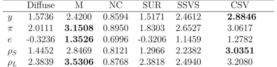
Table 1 and Table 2 present the results of the forecasting exercise. Diffuse refers to a GVAR estimated using maximum likelihood, Minnesota is a standard, homoscedastic GVAR with Minnesota prior, NC denotes a GVAR with natural conjugate prior and SSVS denotes a GVAR with stochastic search variable selection prior. Finally, CSV denotes the GVAR with common stochastic volatility specification.
Table 1: Forecasting Performance, One-Quarter-Ahead: Log Predictive Score
Diffuse M NC SUR SSVS CSV y 1.5736 2.4200 0.8594 1.5171 2.4612 2.8846 π 2.0111 3.1508 0.8950 1.8303 2.6527 3.0617 e -0.3236 1.3526 0.6996 -0.3206 1.1459 1.2782 ρS 1.4452 2.8469 0.8121 1.2966 2.2382 3.0351 ρL 2.3839 3.5306 0.8768 2.3818 2.4940 3.2080
Notes: The figures refer to the average log predictive score specific to variablek. Results based on rolling forecasts over the time period 2010Q1-2012Q4. NC stands for the normal conjugate prior, M stands for the Minnesota prior, SUR stands for the single unit root prior, SSVS stands for the SSVS prior, Diffuse stands for the model estimated using maximum likelihood, CSV stands for the B-GVAR specification with Common Stochastic Volatility. Bold figures refer to the highest value across models for a given endogenous variable.
For real GDP (y), the outperformance in terms of log predictive score is large at the one quarter
ahead time horizon. Comparing columns 5 and 6 of the GDP row in Table 1 reveals that the log predictive score of the CSV specification is around 20 % higher. Furthermore, comparing
2We have computed point forecasts and the results corroborate this statement: The differences in the accuracy
columns 2 and 6 indicates that the CSV specification also improves upon the homoscedastic Minnesota-GVAR to a large extent. In terms of one-year ahead forecasts for real GDP, the CSV is again ahead, outperforming the SSVS specification by around 14 %.
For CPI inflation (π), the prediction gains are less pronounced for the one-quarter ahead time
horizon. Especially when comparing the homoscedastic variant with the CSV specification reveals a small advantage of the linear Minnesota-GVAR, but this difference in terms of log scores is rather negligible. However, comparison with most other specifications reveals that the CSV and Minnesota specifications tend to do well when it comes to forecasting inflation. For the one-year ahead inflation forecasts the Minnesota specification outperforms the CSV specification by around 25%, providing further evidence of strong gains in predictive accuracy when forecasting GDP.
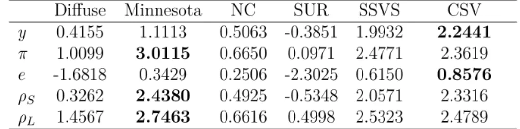
Table 2: Forecasting Performance, One-Year-Ahead: Log Predictive Score
Diffuse Minnesota NC SUR SSVS CSV
y 0.4155 1.1113 0.5063 -0.3851 1.9932 2.2441
π 1.0099 3.0115 0.6650 0.0971 2.4771 2.3619
e -1.6818 0.3429 0.2506 -2.3025 0.6150 0.8576
ρS 0.3262 2.4380 0.4925 -0.5348 2.0571 2.3316
ρL 1.4567 2.7463 0.6616 0.4998 2.5323 2.4789
Notes: The figures refer to the average log predictive score specific to variablek. Results based on rolling forecasts over the time period 2010Q1-2012Q4. NC stands for the normal conjugate prior, M stands for the Minnesota prior, SUR stands for the single unit root prior, SSVS stands for the SSVS prior, Diffuse stands for the model estimated using maximum likelihood, CSV stands for the B-GVAR specification with Common Stochastic Volatility. Bold figures refer to the highest value across models for a given endogenous variable.
One-quarter ahead exchange rate forecasts are surprisingly more accurately forecasted using
the standard Minnesota implementation. As can be seen in the row corresponding to e in
Table 1, Minnesota outperforms its peers by large margins, with the CSV specification showing the second-best performance. This outperformance especially vis-a-vis the CSV specification can be explained by noting that most variables share the same pattern of estimated volatilities, with the exception of the exchange rate. This is a disadvantage of the CSV specification as
compared to specifications where we have ki distinct latent processes in country i. The weak
performance thus is mainly due to a lack of flexibility when it comes to modelling the volatility of real effective exchange rates. However, this does not carry over to the 4-steps ahead exchange rate forecasts. On that time horizon, CSV performs best, closely followed by the SSVS prior specification.
The CSV specification again possesses advantages when used to conduct one-quarter ahead
forecasts of the short-term interest rates (ρS). As compared to its linear counterpart, CSV
outperforms all competitors by large margins. The outperformance against the Minnesota specification is around 19%. For the one-year ahead forecasts the log predictive scores between Minnesota and CSV are comparable, with minor advantages for the homoscedastic variant of
the model. Finally, for long-term interest rates (ρL) the linear Minnesota specification is slightly
ahead for both time horizons considered. This advantage in terms of log scores, however, is negligible. Note that at the one-year ahead horizon the second strongest specification is the SSVS-GVAR, closely followed by the CSV, which ranked third. It is evident that the CSV and Minnesota specifications perform extraordinary well when used to forecast short- and long-term interest rates at both time horizons. This is due to the fact that in financial economics it is typically assumed that those quantities tend to follow random walk processes, which indicates
that a prior that centers the system on a random walk is the best choice to forecast interest rates (see Fama, 1990, for a prominent contribution outlining the difficulty to forecast interest rates at short time horizons).
Comparing the differences between the one- and four-steps time horizon reveals that when used to conduct short-term forecasts, the CSV specification provides increases in predictive accuracy which are significant, especially for GDP and (short-term) interest rate forecasts. However, and
this corroborates the findings in Carriero et al. (2012), for one-year ahead forecasts the CSV
specification has a slight disadvantage when used to forecast inflation and interest rates. This is due to the fact that for longer forecasting horizons, the predicted volatilities approach their long-run mean, implying that the differences in conditional volatilities between the homoscedastic Minnesota-GVAR and the CSV specification disappears.
In our forecasting exercise we have made some efforts to robustify our results with respect to different estimation periods. Some interest results are worth discussing. First, reducing the length of the initial estimation sample (thus effectively including the crisis of 2008/2009 in the hold-out period) leads to qualitatively similar results, although the log predictive scores show significantly more variation over this time period. Furthermore, the inclusion of stochastic volatility helps to robustify the results with respect to the crisis. This implies that over the period 2008 to 2009 the LPS associated to the CSV specification drops significantly less as compared to other specifications.
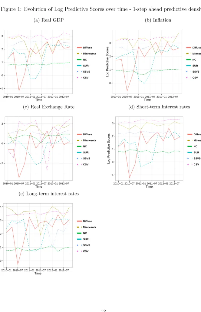
Finally, the inclusion of stochastic volatility should make the forecasts more robust. This implies that in times of economic crisis, stochastic volatility would lead to wider predictive densities, whereas in ”normal” times, the predictive density would be less dispersed. Figure 1 and Figure 2 present the evolution of the log predictive score across different prior structures for the GVAR model. Note that the dashed pink line corresponds to the CSV-specification. Taking a look at the evolution of the LPS for real GDP on both time horizons indicates that the GVAR with stochastic volatility is quite robust, in the sense that it forecasts similarly well during tranquil and crisis times. Comparison with all other specifications, which tend to show a much higher variability of LPS over time, reveals that the CSV specification helps to robustify the analysis with respect to different time periods. This result holds true for all variables under scrutiny, with the exception of the real exchange rate at the one-step ahead time horizon. It can be seen that in that case, the dashed pink line is also quite volatile, dipping below zero twice over the time period 2010Q1 to 2012Q4. Again, the reason here is that due to the single latent process, which also incorporates some information of the variability of the exchange rate equation, is mainly driven by GDP, inflation and both interest rates, which are more homogeneous.
For the year ahead time horizon, it can be seen that the pattern is again similar to the one-step ahead case. However, even though the CSV specification is marginally weaker for interest rates and inflation, the variability over time is lower as compared to most other specifications. Another interesting regularity is that across different variables, the shape of the LPS-curves of different specifications is quite similar, indicating that if a model works well to forecast some variable at a given time, it also works well for other variables at that time. This can be seen by comparing the evolution of log predictive scores for the Diffuse prior specification. For both time horizons, this specification tends to produce weak forecasts for the beginning of the sample (2010Q1 to 2010Q4), but then recovers from 2011Q1 onwards.
Figure 1: Evolution of Log Predictive Scores over time - 1-step ahead predictive density. (a) Real GDP −1 0 1 2 3 2010−01 2010−07 2011−01 2011−07 2012−01 2012−07 Time Log Predictiv e Scores Diffuse Minnesota NC SUR SSVS CSV (b) Inflation 0 1 2 3 2010−01 2010−07 2011−01 2011−07 2012−01 2012−07 Time Log Predictiv e Scores Diffuse Minnesota NC SUR SSVS CSV
(c) Real Exchange Rate
−2 0 2 2010−01 2010−07 2011−01 2011−07 2012−01 2012−07 Time Log Predictiv e Scores Diffuse Minnesota NC SUR SSVS CSV
(d) Short-term interest rates
−1 0 1 2 3 2010−01 2010−07 2011−01 2011−07 2012−01 2012−07 Time Log Predictiv e Scores Diffuse Minnesota NC SUR SSVS CSV
(e) Long-term interest rates
0 1 2 3 4 2010−01 2010−07 2011−01 2011−07 2012−01 2012−07 Time Log Predictiv e Scores Diffuse Minnesota NC SUR SSVS CSV
Figure 2: Evolution of Log Predictive Scores over time - 4-steps ahead predictive density. (a) Real GDP −5.0 −2.5 0.0 2.5 2010−01 2010−07 2011−01 2011−07 2012−01 2012−07 Time Log Predictiv e Scores Diffuse Minnesota NC SUR SSVS CSV (b) Inflation −5.0 −2.5 0.0 2.5 2010−01 2010−07 2011−01 2011−07 2012−01 2012−07 Time Log Predictiv e Scores Diffuse Minnesota NC SUR SSVS CSV
(c) Real Exchange Rate
−7.5 −5.0 −2.5 0.0 2.5 2010−01 2010−07 2011−01 2011−07 2012−01 2012−07 Time Log Predictiv e Scores Diffuse Minnesota NC SUR SSVS CSV
(d) Short-term interest rates
−4 −2 0 2 2010−01 2010−07 2011−01 2011−07 2012−01 2012−07 Time Log Predictiv e Scores Diffuse Minnesota NC SUR SSVS CSV
(e) Long-term interest rates
−4 −2 0 2 4 2010−01 2010−07 2011−01 2011−07 2012−01 2012−07 Time Log Predictiv e Scores Diffuse Minnesota NC SUR SSVS CSV
4.3
Taking a look at the second moment
The previous subsection highlighted the strong, positive effect of stochastic volatility on density forecasting accuracy. The reason why increases in log scores are common for most variables is mainly due to the fact that stochastic volatility allows for another dimension of flexibility, namely accounting for structural changes in the volatility of the underlying time series at the local level. However, because the GVAR framework also allows us to exploit the cross section, one further explanation of this accuracy-premium could be due to information originating from other countries. For example, our framework implicitly allows for contagion effects in terms of rising macroeconomic volatility, which implies that cross-sectional information is exploited efficiently. This is achieved by noting that other countries influence domestic volatility through the inclusion of weakly exogenous factors. As a consequence, our model succeeds in exploiting
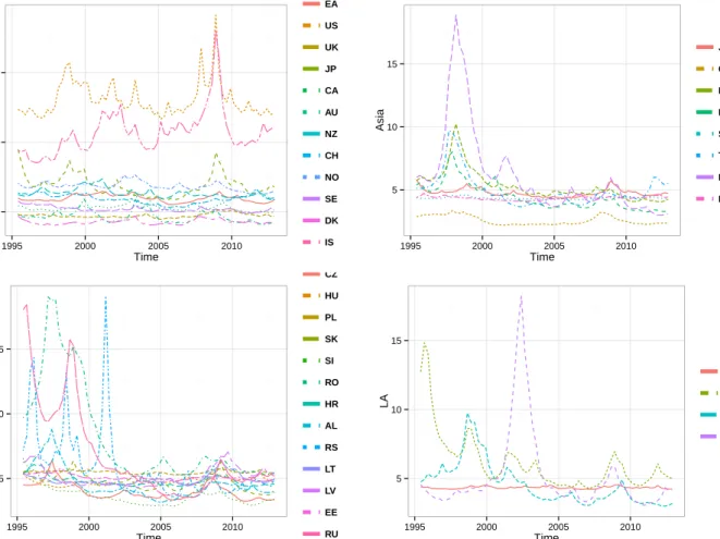
Figure 3: Posterior Mean of country specific standard deviations over time
4 6 8 1995 2000 2005 2010 Time Rest EA US UK JP CA AU NZ CH NO SE DK IS 5 10 15 1995 2000 2005 2010 Time Asia JP CN KR PH SG TH ID IN 5 10 15 1995 2000 2005 2010 Time EEU CZ HU PL SK SI RO HR AL RS LT LV EE RU 5 10 15 1995 2000 2005 2010 Time LA CL MX PE AR
this information and translates this into stronger forecasting performance. It is evident that
some countries tend to react faster to economic shocks then other countries. In terms of
forecasting this would imply that if country j experiences a sudden rise in volatility at time
t+h, countryi would also be influenced at timet+h through the weakly exogenous factors.
This would contemporaneously affect the predictive densities in country i, leading to wider
prediction intervals.
Figure 3 presents the posterior mean of country specific volatilities across country groups for selected economies. Note that our model succeeded in finding most significant economic events
in all countries under scrutiny. This includes the economic crises in Argentina and Russia, the Asian crisis and for the developed economies the recent downturn of 2008/2009. Furthermore, within-group-volatility appears to be quite homogeneous. This implies that most economies within a group tend to follow the same pattern in terms of volatility dynamics.
5
Conclusion and Further Remarks
This paper has shown that adding stochastic volatility to the GVAR modelling framework tends to improve the accuracy of density forecasts by large margins. Furthermore, as expected, stochastic volatility specifications tend to produce more robust predictions with respect to the underlying forecasting period. Our GVAR with common stochastic volatility improves upon a battery of linear Bayesian GVARs for several variables under scrutiny at the one-quarter ahead time horizon, with the main exception being the real effective exchange rates. This result is mainly due to the heterogeneous nature of exchange rate volatility as compared to GDP, in-flation and interest rate volatility. Thus, to further increase the predictive capabilities when it comes to forecasting real exchange rates it might be needed to introduce more flexibility and allow for different stochastic processes across the variables within the local level models. The results found for the one-quarter ahead horizon carry over to the one-year ahead horizon. For predicting GDP and interest rates, the CSV specification is still the best model, whereas infla-tion and real exchange rates it falls behind its homoscedastic counterpart, the linear Minnesota specification. To account for the prevailing heterogeneity observed in the world economy it would also be possible to replace the Minnesota prior used for the CSV specification with a hierarchical SSVS prior specification. This could combine the virtues of a specification which is robust towards heteroscedasticity and a specification which accounts for model uncertainty at the individual country level. As a possible avenue of further research the inclusion of time varying dynamic coefficients could also prove to have a positive influence on the accuracy of point and density forecasts.
References
Bańbura, M., D. Giannone, & L. Reichlin (2010): “Large bayesian vector auto regressions.” Journal of
Applied Econometrics25(1): pp. 71–92.
Carriero, A., T.Clark, & M.Marcellino(2012): “Common drifting volatility in large bayesian vars.” . Carriero, A., G.Kapetanios, & M.Marcellino(2009): “Forecasting exchange rates with a large Bayesian
VAR.” International Journal of Forecasting 25(2): pp. 400–417.
Cesa-Bianchi, A., M. H. Pesaran, & A. Rebucci (2014): “Uncertainty and economic activity: A global perspective.” Technical report, CESifo Working Paper.
Clark, T. E. (2011): “Real-time density forecasts from bayesian vector autoregressions with stochastic volatil-ity.” Journal of Business & Economic Statistics29(3).
Crespo Cuaresma, J. C., M.Feldkircher, & F.Huber (2014): “Forecasting with bayesian global vector autoregressive models: A comparison of priors.” Technical report.
Dees, S., F.di Mauro, H. M.Pesaran, & L. V. Smith(2007): “Exploring the international linkages of the euro area: a global VAR analysis.” Journal of Applied Econometrics 22(1).
Eisenstat, E. & R. W.Strachan(2014): “Modelling inflation volatility.”Technical report, Centre for Applied
Macroeconomic Analysis, Crawford School of Public Policy, The Australian National University.
Fama, E. F. (1990): “Term-structure forecasts of interest rates, inflation and real returns.”Journal of Monetary
Economics25(1): pp. 59–76.
Feldkircher, M. (2013): “A Global Macro Model for Emerging Europe.” Oesterreichische Nationalbank Working Paper Series185/2013.
Frühwirth-Schnatter, S. & H. Wagner (2010): “Stochastic model specification search for gaussian and partial non-gaussian state space models.” Journal of Econometrics 154(1): pp. 85–100.
Giordani, P. & M. Villani (2010): “Forecasting macroeconomic time series with locally adaptive signal extraction.” International Journal of Forecasting 26(2): pp. 312–325.
Greenwood-Nimmo, M., V. H. Nguyen, & Y. Shin (2012): “Probabilistic Forecasting of Output Growth, Inflation and the Balance of Trade in a GVAR Framework.”Journal of Applied Econometrics27: pp. 554–573.
Kadiyala, K. & S. Karlsson (1997): “Numerical methods for estimation and inference in bayesian
var-models.” Journal of Applied Econometrics12(2): pp. 99–132.
Karlsson, S. (2012): “Forecasting with Bayesian Vector Autoregressions.” Örebro University Working Paper
12/2012.
Kastner, G. & S. Frühwirth-Schnatter (2013): “Ancillarity-sufficiency interweaving strategy (asis) for
boosting mcmc estimation of stochastic volatility models.” Computational Statistics & Data Analysis.
Koop, G. & D.Korobilis(2013): “Large time-varying parameter vars.” Journal of Econometrics 177(2): pp. 185–198.
Koop, G. M. (2013): “Forecasting with medium and large bayesian vars.” Journal of Applied Econometrics
28(2): pp. 177–203.
Pesaran, M. H., T. Schuermann, & L. V. Smith (2007): “What if the UK or Sweden had joined the euro in 1999? An empirical evaluation using a Global VAR.” International Journal of Finance and Economics
12(1): pp. 55–87.
Pesaran, M. H., T.Schuermann, & L. V.Smith(2009): “Forecasting economic and financial variables with
global VARs.” International Journal of Forecasting 25(4): pp. 642–675.
Pesaran, M. H., T.Schuermann, & S. M.Weiner(2004): “Modeling Regional Interdependencies Using a
Global Error-Correcting Macroeconometric Model.” Journal of Business and Economic Statistics, American Statistical Association 22: pp. 129–162.
Zellner, A. (1976): “Bayesian and non-bayesian analysis of the regression model with multivariate student-t error terms.” Journal of the American Statistical Association 71(354): pp. 400–405.
A
Data Appendix
Advanced Economies (11): US, EA, UK, CA, AU, NZ, CH, NO, SE, DK, IS
Emerging Europe (14): CZ, HU, PL, SK, SI, BG, RO, HR, AL, RS, TR, LT, LV, EE
CIS and Mongolia (6): RU, UA, BY, KG, MN, GE
Asia (9): CN, KR, JP, PH, SG, TH, ID, IN, MY
Latin America (5): AR, BR, CL, MX, PE
Middle East and Africa (1): EG
Abbreviations refer to the two-digit ISO country code. Source: Feldkircher (2013)
Table 3: Country coverage
Table 4: Data description
Variable Description Min. Mean Max. Coverage
y Real GDP, average of
2005=100. Seasonally
adjusted, in logarithms.
3.465 4.516 5.194 100%
π Consumer price inflation.
CPI seasonally adjusted, in logarithms.
-0.258 0.020 1.194 100%
e Nominal exchange rate
vis-à-vis the US dollar, de-flated by national price lev-els (CPI).
5.699 -2.220 5.459 97.8%
ρS Typically 3-months-market
rates, rates per annum.
0.000 0.100 4.332 93.5%
ρL Typically government bond
yields, rates per annum.
0.006 0.060 0.777 39.1%
poil Price of oil, seasonally
ad-justed, in logarithms.
- - -
-Trade flows Bilateral data on exports
and imports of goods and services, annual data.
- - -
-Summary statistics pooled over countries and time.
The coverage refers to the cross-country availability per country, in %. Source: Feldkircher (2013).