A Break-even Analysis of RFID Technology for Inventory sensitive to Shrinkage

(1)

A Break-even Analysis of RFID Technology

for Inventory sensitive to Shrinkage

A.G. de Kok, K.H. van Donselaar, T. van Woensel

∗

TU/e Eindhoven University of Technology Department of Technology Management Den Dolech 2, NL5600 MB Eindhoven, The Netherlands

Abstract

By embedding RFID tags onto their products, both manufacturers and retailers try to control for shrinkage (e.g. due to theft). Current inventory control systems do not take into account the disappearing inventory due to this shrinkage. As a response, corrective actions are made by performing costly audits in which actual inventory is counted. The research presented in this paper adapts the inventory policy by including both the shrinkage fraction and the impact of RFID technology. Accordingly, by comparing the situation with RFID and the one without RFID in terms of costs, an exact analytical expression can be derived for the break-even prices of an RFID tag. It turns out that these break-even prices are highly related with the value of the items that are lost, the shrinkage fraction and the remaining shrinkage after implementing RFID. A simple rough-cut approximation to determine the maximum amount of money a manager should be willing to invest in RFID technology is presented and evaluated.

Key words: Inventory control, Shrinkage, RFID, Break-even analysis

1. Introduction

More and more, RFID technology is expected to take the place of bar codes in the supply chain allowing manufacturers and retailers to know the exact location and quantity of their inventory without conducting time consuming audits at several points along the chain. Assuming that the detection equipment is reasonable reliable, RFID should provide more accurate information of the available inventories and its position throughout the

∗ _{Corresponding author}

Email addresses:[email protected] (A.G. de Kok),[email protected] (K.H. van Donselaar),[email protected](T. van Woensel).

(2)

chain. McFarlane and Sheffi (2003) reviewed some of the key challenges of RFID in supply chain operations and introduced the main elements of using such a system. The problem is however that this technology is perceived as expensive and therefore not (yet) feasible. This paper establishes a cost-benefit trade-off, generating exact analytical expressions for the break-even RFID prices, as such facilitating business case calculations.

Atali et al. (2005) distinguish in their paper between three main sources of inventory discrepancies which are not taken into account in the classical inventory models:

(i) Shrinkage: thefts are generally not captured by the inventory control. As such, this leads to a system inventory which is higher than the actual inventory.

(ii) Misplacement of products: goods are not in the correct place and are thus not avail-able for customers. Consequently, inventory is correct but partially not availavail-able, introducing an inventory deviation.

(iii) Transaction errors: this is related to wrong scanning of products at the check-out counters in retail outlets or switches of products in the suppliers warehouse. The standard way of identifying and remedying for the above inventory deviations is doing costly audits. As such, both physical errors (e.g. misplaced items) as system in-ventory errors (e.g. due to shrinkage or transaction errors) are corrected for. Complete and accurate information on the inventory status in the supply chain is thus crucial. In this paper, we mainly focus on the inventory inaccuracy caused by shrinkage.

Our application assumes that, depending upon the achieved read accuracy, RFID en-hances the accuracy of the information currently obtained through bar code scanning which is more vulnerable to human error. Consequently, we assume that RFID results in a better control of shrinkage. Shrinkage can then either be completely vanished (i.e. 100% reliable RFID), or some fraction of the shrinkage observed in the situation before RFID was used, is left (RFID is less than 100% reliable, e.g. due to read errors). The latter case seems to be more realistic: Lee and Ozer (2005) report that between 10% and 66% of the original shrinkage observed is reduced after implementing RFID technologies. When having this shrinkage information, one however should take this information into account when determining the stock levels. Traditional inventory management literature assumes that inventory managers know exactly what they are storing and that this information is 100% reliable. In reality, due to e.g. shrinkage inventory records are only rough estimates of the actual inventory on the retail shelves or in the manufacturer’s warehouse. A contribution of this paper is that we determine an inventory policy taking into account shrinkage.

Today, a substantial amount of empirical research on inventory discrepancy is avail-able. DeHoratius et al. (2004) found that 65% of the inventory records at one retailer were inaccurate. Along the same line, Kang and Gershwin (2005) found that the best performing store in their sample study only had 70-75% of its inventory record matching physical inventory during its annual inventory audit. The overall average over all stores was 51%. Raman et al. (2001b) reported that, at the stores of one retailer, two-thirds of the Stock Keeping Units (SKUs) had inaccurate inventory records upon physical audits. Such inaccuracies could have the potential of reducing profit by 10% due to higher inven-tory cost and lost sales. Other studies report that the main cause of inveninven-tory discrepancy is due to shrinkage: Fleisch and Tellkamp (2005) reported that shrinkage accounted for 2-4% of sales in the US retail industry in 2001. Alexander et al. (2002) at IBM reported that the amount of inventory shrinkage rates are around 1.75% of 2001 sales in the US, Europe and Australasia. ECR Europe (2003) found that, in Europe, the shrinkage rates

(3)

were 1.75% for retailers and 0.56% for manufacturers.

In general, literature on an analytical assessment of the RFID technology is fairly limited. Atali et al. (2005) and Lee and Ozer (2005) mainly focus on the inventory function and the effect of taking into account the inventory discrepancy. It is however stated that a cost-benefit trade-off for RIFD tags is still an open issue not tackled by their research. In another paper, Kok and Shang (2005), assume in their model that inventory errors are i.i.d with a mean of zero. In this setting, they model the transaction-and misplacement errors but not the shrinkage errors. They state that the commonly practiced audit policies can only be effective if the right inspection cycle is chosen. They however did not optimize on this inspection cycle length for the audits in their study. Rekik et al. (2005) model the consequences of misplacement of inventory on the retail shelf by comparing three alternatives. In the first alternative, the retailer is unaware of the misplacement and places his orders as if inventory information is perfect. In the second case, the retailer is aware of the errors in his inventory status information, and adjusts his ordering policy accordingly. In the final scenario, perfect inventory status information based on RFID technology is assumed. The problem is modeled using a conventional newsboy formulation with some modifications to adjust for the scenarios described above. A numerical analysis demonstrates the limited benefits of RFID.

Our paper positions itself close to these literature contributions. More specifically, it focuses on the cost-benefit trade-off between inventory costs and the costs of RFID with regards to shrinkage (as such extending the analysis in Atali et al. (2005)). Next to this, the length of the inspection cycle is explicitly taken into account in the analysis. This was a parameter that needs to be optimized as indicated by the research of Kok and Shang (2005) (they considered in their paper the inspection cycle length as given). Compared to Rekik et al. (2005) model, we use a more appropriate inventory model (i.e. a periodic review base stock policy) rather than the single period newsboy model of which the use is mainly limited to e.g. fashion products.

The overall objective of this paper is to determine the additional cost per time unit caused by shrinkage. One might then consider RFID equipment and tag investments that in principle allow to prevent shrinkage and to come to (almost) perfect observation (i.e. benefits), yet at the expense of additional investments in equipment and tags (i.e. costs). The insights in this paper are not limited to RFID only but are also useful for any technology cost-benefit analysis with inventory implications.

This paper makes the following contributions:

– Current inventory base stock policies are augmented taking into account inventory shrinkage. As such, we quantify the potential gains of using any technology (e.g. RFID) leading to better knowledge on the actual inventory status. The approach is flexible as it also considers residual shrinkage after implementing RFID. As such, it takes into account potential problems (e.g. read errors) occurring after RFID implementation. – The analysis presented gives a detailed cost-benefit analysis focusing on the most

relevant factors (e.g. the cost of the technology, the inspection cycle length, etc.). This results in exact analytical expressions for the break-even RFID prices.

– The effect of the length of the inspection cycle is explicitly taken into account, quan-tified and optimized. It is shown that the inspection cycle has an important effect on the behavior of the break-even prices.

– Finally, it is shown that the value of the item, the fraction of demand that is dis-appeared and the remaining shrinkage after RFID implementation have the largest

(4)

impact on the break-even prices for the RFID tags (when the inspection cycle length is optimized). A simple rough-cut approximation is presented to calculate the break-even prices.

This paper is organized as follows: in the next section the model is developed and ex-act expressions for the break-even prices are derived, then computational results are presented for a complete experimental design; the last section concludes the paper. 2. Model development

Before starting with the analysis, we summarize in Table 1 the variables used in the analysis.

We assume a periodic review base stock policy: every R periods, the inventory is reviewed and raised to an order-up-to levelS (see also e.g. Silver et al. (1998) for more information on the stock policy used). Demand in subsequent periods isi.i.d.; letE[D] denote the expected demand per period and assume that a fraction of demand per period, Π disappears due to shrinkage, misplacement, etc. The disappeared stock is lost. We assume that demand not met from the shelf is backordered and assume that the process of disappearances is pure Poisson with rateλs= ΠE[D]. Hence total consumption per

time unit equals (1 + Π)E[D].

At each review moment, the observation of the inventory takes place. We assume that inventories are counted then for a random sample of stock keeping units (SKUs). The probability that a particular SKU is in this sample is set equal top. Consequently, with this probabilitypthe disappearance of items is identified correctly and with probability (1−p) the inventory is based on the inventory at the last review moment minus observed demand plus replenishment arriving between the last review moment and the current one.

DefineCas the length of an observation cycle, i.e. the number of periods between two review moments at which the inventory is observed correctly. Then it follows that:

P(C=k) =p(1−p)k−1, k= 1,2, ... (1) Consequently, the expected observation cycle lengthE[C] is then equal to:

E[C] = 1

p (2)

From renewal reward theory (Tijms Tijms (2003)), we find the following identities: E[X] = P∞ k=1p(1−p) k−1Pk j=1E[Xjk] E[C] (3) E[B] = P∞ k=1p(1−p) k−1Pk j=1E[Bjk] E[C] (4)

Suppose that at time 0 the inventory is perfectly observed, i.e. an observation cycle starts. Suppose that this cycle has lengthk. Let us consider thej-th review moment in this cycle 1≤j≤k, with the first review moment at time 0. Immediately after that moment the actual inventory position is equal toS−D2(0,(j−1)R] , while the inventory control function assumes that the inventory position equals S. The order generated at time

(5)

Table 1

List of variables used in the analysis Variable Description

C Observation cycle length

1/p Expected observation cycle length

1/pnoRF IDExpected observation cycle length without RFID 1/pRF ID Expected observation cycle length with RFID

E[D] Expected demand per period Π Disappearance fraction λs The rate of disappearances

Xjk Physical inventory at the end of thej-th replenishment cycle associated with observation cycle of lengthk, just before the next order is delivered

Bjk Amount of the demand backordered during thej-th

replenishment cycle associated with observation cycle of lengthk X Value of the physical inventory at the end of an

arbitrary period, just before an order is delivered B Value of the amount of demand backordered

during an arbitrary period D1(s, t] Demand during the interval (s, t]

D2(s, t] Disappearances during the interval (s, t]

R Length of the review period

Lj Lead time for thej-th order in an observation cycle

S Order-up-to level

Nr Number of periods per year

v Price per unit of the product sold δ Auditing costs

r Annual interest rate

α Fraction of Π that cannot be prevented from disappearing

θ Tag costs

(j−1)Ris received at time (j−1)R+Lj, withLj the leadtime of thej-th order in the

observation cycle. Thus the actual net inventory at moment (j−1)R+Lj, immediately

after arrival of this order, denoted byNa

j−1,k, equals:

Nja−1,k =S−D2(0,(j−1)R+Lj]−D1((j−1)R,(j−1)R+Lj]

Likewise, the actual net inventory justbefore the arrival of the next order (placed at timejRand due at timejR+Lj+1), denoted by N_j,kb is equal to:

Nb

(6)

Using the above expressions for the net inventory and the fact thatXjk=Max(Nj,kb ,0)

andBjk= (Max(−Nj,kb ,0)−Max(−N a

j−1,k,0)), we find the following equations:

E(Xjk) =E h (S−D2(0, jR+Lj+1]−D1((j−1)R, jR+Lj+1])+ i E(Bjk) =E h (D2(0, jR+Lj+1] +D1((j−1)R, jR+Lj+1]−S)+ i −Eh(D2(0,(j−1)R+Lj] +D1((j−1)R,(j−1)R+Lj]−S)+ i

Define the following auxiliary variables to simplify the notation: Zj1=D2(0, jR+Lj+1] +D1((j−1)R, jR+Lj+1] Zj2=D2(0,(j−1)R+Lj] +D1((j−1)R,(j−1)R+Lj] ⇒E[Xjk] =E h (S−Zj1) +i ⇒E[Bjk] =E h (Zj1−S)+ i −Eh(Zj2−S)+ i

Then it follows that: E[X] =p ∞ X k=1 p(1−p)k−1 k X j=1 E[Xjk] =p ∞ X k=1 p(1−p)k−1 k X j=1 Eh(S−Zj1) +i =p ∞ X j=1 ∞ X k=j p(1−p)k−1Eh(S−Zj1) +i =p ∞ X j=1 Eh(S−Zj1)+ i p(1−p)j−1 ∞ X k=0 (1−p)k = ∞ X j=1 p(1−p)j−1Eh(S−Zj1) +i (5) Similarly, the following expression forE[B] can be obtained:

E[B] = ∞ X j=1 p(1−p)j−1Eh(Zj1−S)+ i −Eh(Zj2−S)+ i (6) We remark here that the expressions forEh(Zj1−S)+

i

andEh(Zj2−S)+ i

can rou-tinely be calculated ifZj1andZj2are assumed to be mixed-Erlang distributed (see e.g. Tijms (2003)).

LetP2 be the long-run fraction of the demand filled directly from the stock on-hand, then it follows that:

P2= 1− E[B]

(7)

Let Nr denote the number of periods per year. Let us assume that the price of the

product sold equals v and the annual interest rate equalsr . So the inventory holding costs arev×r(euro per unit per year) times the average number of units in the pipeline or on hand. The cost of auditing the inventory equalsδ. LetE[L] be the expected leadtime of an order, then the total relevant annual costs,T RCnoRF ID, are equal to:

T RCnoRF ID =vr(1 + Π)E[D]E[L] +vrE[XnoRF ID]

+vΠE[D]Nr+δpnoRF IDNr (8)

These costs are the sum of all the relevant cost components involved:

(i) Inventory costs, being the costs for the pipeline stock, vr(1 + Π)E[D]E[L] and for the average inventory on hand,vrE[XnoRF ID]

(ii) Shrinkage costs:vΠE[D]Nr

(iii) Audit costs:δpnoRF IDNr

Similarly, we can construct the total relevant annual costs under RFID (denoted as, T RCRF ID). Assume that RFID has the potential to eliminate shrinkage but might leave

some fractionαof Π (0≤α≤1) that cannot be protected from shrinkage. In other words, the shrinkage left after implementing RFID will be between 0 (α= 0, i.e. 100% reduction) and Π (α= 1, i.e. no reduction of shrinkage through RFID). Using the αfactor we can thus control for the expected shrinkage when using RFID. The total relevant costs using RFID withθ the cost of the RFID tag is composed of the following cost components:

(i) Inventory costs, being the combination of costs for the pipeline inventoryvr(1 +αΠ)E[D]E[L] and for the average inventory on hand,vrE[XRF ID].

(ii) Shrinkage costs:vαΠE[D]Nr

(iii) Tag costs:θE[D]Nr

(iv) Audit costs:δpRF IDNr|(α6=0)

As one can see, the costs depend on the value of α: if α = 0, then RFID is 100% reliable so that audit costs can be dropped. Ifα6= 0, then audits are still necessary to periodically correct the inventory records. This might be due to e.g. read errors with the RFID equipment, etc. Note that the specific physical inventory depends on the use of RFID (E[XRF ID]) or not (E[XnoRF ID]) and onα. The inventory level (E[XRF ID])

needed to guarantee the service level will be higher (compared to the α= 0 case). On top of this inventory increase, we will face extra costs due to shrinkage at a rate ofαΠ.

The total relevant annual costs under RFID are then equal to: T RCRF ID=vr(1 +αΠ)E[D]E[L] +vrE[XRF ID]

+vαΠE[D]Nr+θE[D]Nr+δpRF IDNr|(α6=0) (9) Ifα= 0 (i.e. assuming 100% reduction of shrinkage), Equation (9) reduces to:

T RCRF ID=vrE[D]E[L] +vrE[XRF ID] +θE[D]Nr (10)

Comparing Equations (8) and (9), we find that the no-RFID situation is more costly than the RFID situation (in the case that the observation cycle length is the same in both situations) if and only if:

(8)

T RCnoRF ID > T RCRF ID (11)

⇔

vr(1 + Π)E[D]E[L] +vrE[XnoRF ID] +vΠE[D]Nr+δpnoRF IDNr

> vr(1 +αΠ)E[D]E[L] +vrE[XRF ID] +vαΠE[D]Nr +θE[D]Nr+δpRF IDNr|(α6=0) (12) Or equivalently: vr(1−α) ΠE[D]E[L] +vr(E[XnoRF ID]−E[XRF ID]) +v(1−α) ΠE[D]Nr −θE[D]Nr+ δpnoRF IDNr−δpRF IDNr|(α6=0) >0 (13)

Again ifα= 0, then the termδpRF IDNr|(α6=0)equals zero and can be dropped; in the other case where the fractionα6= 0, some residual shrinkage is left from Π after RFID implementation and we again have to take into account the audit costs under RFID. Expressing this inequality as a constraint on θ, we find that RFID is profitable if the following condition holds:

v(1−α) Π +vr(1−α) ΠE[L] Nr +vr(E[X]−E[XRF ID]) NrE[D] + _δp noRF ID E[D] − δpRF ID E[D] |(α6=0) > θ (14)

If α= 0, then the termδpRF IDNr|(α6=0) equals zero and can be dropped. Note that thepRF ID is not necessarily the same as thepnoRF ID. In Section?? we will look more

closely on the optimalpfor each of the two situations. If RFID is 100% reliable then the above equation reduces to:

vΠ +vrΠE[L] Nr +vr(E[X]−E[XRF ID]) NrE[D] +δpnoRF ID E[D] > θ (15) In the next section, the exact analytical expression for the break-even prices in Equa-tion (14) will be evaluated for a large number of settings.

3. Experimental results

3.1. Experimental design and Methodology

To analyze the effect of the different parameters on the expected break-even prices, we perform a closed experimental design (see e.g. Law and Kelton (2000)). The demand in the analysis is based on fitting a mixed Erlang distribution (see e.g. Tijms (2003)); the number of periods per yearNr, is set equal to 250. The observation cycle lengths 1/pin

Table 2 correspond to checking once a week (1/p= 5), once in four weeks (1/p= 20), once in 12 weeks (1/p= 60) and once a year (1/p= 250). The value of an itemvis chosen such that there are cheap items (e.g. 1 euro, which is typically the average price in grocery retailing, see e.g. van Donselaar et al. (2004)) and expensive items (in this paper set to 20 euro) in our experimental design. The other values in the table are inspired on Atali

(9)

et al. (2005) and Lee and Ozer (2005) and chosen such that the experimental design is complete and balanced. Combining all these values for the specific parameters, resulted in an extensive dataset including 62,208 observations, (in which each observation refers to a specific parameter setting, its resulting costs and the break-even price obtained to reach the pre-definedP2).

Table 2

Experimental design

Parameter used Values

Π Theft fraction {0.01,0.02,0.05,0.2}

v Value of an item {1,20}

r Annual interest rate {0.1,0.2}

E(D) Expected demand {0.2,1,5}

CV(D) Coefficient of variation demand {0.1,0.5,1}

L Lead time {1,5,20}

P2 Target fill rate {0.90,0.95,0.99}

δ Audit costs {0.25,0.75,1.50}

1/p Observation cycle length {week, 4 weeks, 12 weeks, year}

α Fraction of theft that cannot be{0,0.25,0.50,0.75}

solved by using RFID

The analysis is performed in a number of consecutive steps: first, we analyze the complete data set and identify the main drivers of the break-even prices (Section 3.2). Secondly, we reduce the dataset by optimizing over the observation period, i.e. we select the best setting for each parameter combination which is minimezed for the observation cycle length on the total relevant cots. This reduced dataset is then analyzed in detail (Section 3.3). Finally, we present and evaluate a simple approximation for the break-even prices based on the analysis (Section 3.4).

3.2. Overall analysis

The average break-even prices for each of the parameters and its specific value are presented in Table 3. Each column represents a different value forα, i.e. in the case where α = 0.50, 50% of the original theft fraction Π remains unresolved after implementing RFID.

An analysis of the range of all the parameters shows that the break-even prices vary significantly with the theft fraction, Π and the value of the item,v. For the other param-eters in the analysis the effect is less pronounced. Next to this,αalso has an important impact on the break-even prices: comparing horizontally one can observe in all cases a significant effect of changingα.

Finally, note that for the observation cycle length 1/p a significant effect can be ob-served (for allαvalues). Especially for α= 0, we observe aU-shape effect. This is due to the interaction effect of the inventory costs and the audit costs averaged over all ob-servations. For the otherαvalues this effect is distorted by the extra addition of audit

(10)

Table 3

Break-even prices (in euro) for all parameters Break-even price (in euro) Parameter Value α= 0.00α= 0.25α= 0.50α= 0.75 Π 0.01 0.2335 0.0877 0.0586 0.0293 0.02 0.3511 0.1762 0.1176 0.0588 0.05 0.7045 0.4416 0.2946 0.1473 0.20 2.4731 1.7685 1.1791 0.5895 v 1.00 0.1950 0.0589 0.0393 0.1964 20.00 1.6861 1.1781 0.7856 0.3929 r 0.10 0.9109 0.0084 0.0056 0.0028 0.20 0.9702 0.6409 0.4274 0.2137 E(D) 0.20 1.1173 0.6234 0.4151 0.2074 1.00 0.8768 0.6169 0.4116 0.2059 5.00 0.8275 0.6152 0.4107 0.2055 CV(D) 0.10 0.9481 0.6215 0.4139 0.2068 0.50 0.9408 0.6189 0.4127 0.2064 1.00 0.9328 0.6151 0.4107 0.2055 E(L) 1 0.9393 0.6170 0.4113 0.2056 5 0.9395 0.6175 0.4117 0.2059 20 0.9428 0.6210 0.4143 0.2072 P2 0.90 0.9056 0.5922 0.3949 0.1975 0.95 0.9291 0.6099 0.4067 0.2034 0.99 0.9871 0.6534 0.4357 0.2178 δ 0.25 0.8589 0.6185 0.4124 0.2062 0.75 0.9289 0.6185 0.4124 0.2062 1.50 1.0338 0.6185 0.4124 0.2062 1/p week 1.0898 0.5586 0.3723 0.1861 4 weeks 0.8446 0.5688 0.3793 0.1896 12 weeks 0.8268 0.5992 0.3997 0.1999 year 1.0009 0.7475 0.4986 0.2494

costs due to the imperfect observation (e.g. due to the read rate). The observation cycle length does have a big impact on the results: Table 4 shows the effect of the total relevant costs depending on the observation cycle length and the value of the items that gets lost, i.e. Πv. We use the latter value as it is a good representation of the two extreme ”high value-high theft” (Πv= 4) and ”low value-low theft” (Πv= 0.01) situations. The ”All” situation refers to the costs averaged out over all observations without clustering based on Πv. The Total Relevant Costs are equal here to the sum of the inventory costs and the audit costs since all other costs in Equation (8) do not depend on the length of the

(11)

Table 4

Observation length effect on the average inventory and average audit costs Observation cycle length

Πv Costs (in euro) year 12 weeks 4 weeks week 0.01 Inventory Costs 4.86 3.77 3.62 3.56

Audit Costs 0.83 3.48 10.41 41.67 Total Relevant Costs 5_.69 ₇_.₂₅ ₁₄_.₀₄ ₄₅_.₂₅

4.00 Inventory Costs 794.92 240.80 126.83 89.93 Audit Costs 0.83 3.48 10.42 41.67 Total Relevant Costs 795.75 244.28 137.25131_.60

All Inventory Costs 166.05 66.12 46.62 40.64 Audit Costs 0.83 3.48 10.42 41.67 Total Relevant Costs 166.89 69.60 57_.04 ₈₂_.₃₁

observation cycle.

Concluding, it can be observed that if a long observation cycle is chosen, the inven-tory investment increases dramatically. Table 4 indicates the importance of choosing the correct observation cycle length depending upon the specific value of the itemv and the theft rate Π. Note that theU-shape effect on the total costs in theAllsituation is due to the interaction effect of the inventory costs and the audit costs without separating the cases based on Πv. High value items with a high theft rate should be counted weekly, i.e. the total costs are minimal for this case (131.60 euro). Low value items with a low theft rate can suffice with only counting once a year (with total costs equal to 5.69 euro). The table also shows that if the wrong observation cycle length is chosen, the costs increase dramatically. Based on this table, we conclude that the observation cycle length is an important parameter that needs to be optimized (i.e. confirming the conclusion of Kok and Shang (2005) on the need to optimize the observation cycle length).

3.3. Analysis with the optimized observation cycles

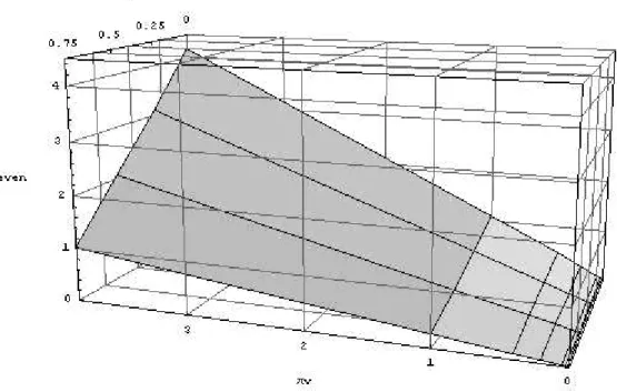
In our dataset of 62,208 observations, we have four observations for each parameter combination, each with a different observation cycle length. In this dataset, we now select the lowest total relevant costs for each of these four parameter combinations, resulting in a reduced dataset of 15,552 observations which are optimal in terms of the observation cycle length. Figure 1 shows the average over all optimal observation cycles (1/p) for all combinationsαand Πv. The figure shows that high value items with high theft are more likely to be audited more than cheap items with low theft. Moreover, if the remaining theft rate α is not too high, it is cost optimal to do less frequent auditing than with higherα. Do note that the case whereα= 1 refers to the no-RFID situation.

To see the effect of this optimization step, we again show the sensitivity of each pa-rameter with regards to the average break-even price in Table 5. The break-even price is now determined from:

(12)

Fig. 1. Optimal observation period for all combinationsαand Πv v(1−α) Π +vr(1−α) ΠE[L] Nr +vr(E[X]−E[XRF ID]) NrE[D] + _δp∗ E[D]− δp∗∗ E[D]|(α6=0) > θ (16)

In this equation,p∗_and_p∗∗_{are the optimized observation cycles for the no-RFID resp.} the RFID (α6= 0) situation in terms of the minimized total relevant costs for the no-RFID versus the RFID case. Do note that depending upon the cost structure, we might get two different optimal observation cycles. Depending upon the specific parameter settings it might be optimal to do more or less audits in the RFID case whereα6= 0 compared to the no-RFID situation.

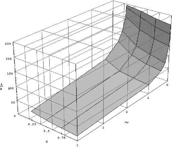
The main effects as originally observed in Table 3 stay the same, only the importance of the relevant parameters (i.e. the theft fraction, Π, the value of the item, v and the remaining theft fractionα) compared to the other parameters, has increased even further. In the subsequent analysis, we will focus more on the specific relationship between Π, v and α. Figure 2 shows the optimal break-even prices for all possible combinations of α

(13)

Table 5

Break-even prices (in euro) for each parameter (optimized scenarios) Break-even price (in euro)

Parameter Valueα= 0.00α= 0.25α= 0.50α= 0.75 Π 0.01 0.1291 0.0895 0.0589 0.0292 0.02 0.2434 0.1732 0.1143 0.0567 0.05 0.5774 0.4195 0.2779 0.1384 0.20 2.2118 1.6344 1.0858 0.5417 v 1.00 0.0897 0.0609 0.0402 0.0199 20.00 1.4911 1.0973 0.7282 0.3631 r 0.10 0.7803 0.5736 0.3809 0.1900 0.20 0.8006 0.5847 0.3875 0.1929 E(D) 0.20 0.8432 0.6025 0.3979 0.1978 1.00 0.7762 0.5734 0.3809 0.1901 5.00 0.7519 0.5615 0.3737 0.1867 CV(D) 0.10 0.7969 0.5810 0.3852 0.1919 0.50 0.7903 0.5793 0.3842 0.1915 1.00 0.7840 0.5771 0.3831 0.1910 E(L) 1 0.7882 0.5768 0.3826 0.1906 5 0.7893 0.5778 0.3833 0.1911 20 0.7937 0.5827 0.3867 0.1928 P2 0.90 0.7789 0.5732 0.3808 0.1900 0.95 0.7876 0.5778 0.3835 0.1912 0.99 0.8046 0.5864 0.3883 0.1933 δ 0.25 0.7691 0.5692 0.3783 0.1888 0.75 0.7902 0.5791 0.3840 0.1913 1.50 0.8119 0.5891 0.3902 0.1943 and Πv.

From Figure 2 it is clear that there is a significant influence from bothαand Πvon the break-even prices. For high Πv(left hand in the figure), break-even prices reduce almost linear as a function of α. Similar, for low Πv one might come to the same conclusion. However, as the numbers are extremely small in this region, we also present the table with some relevant key numbers. Table 6 shows the break-even prices spread over the different demand rates for the optimized observation cycle length.

Looking at the ”Overall” row in Table 6, we see that for Πv = 0.01 (i.e. low) that the relationship with αis not linear, while for Πv= 4.00 it is closer to linear. In other words, if after implementation the read rate would not lead to 100% correct information, the effect on the break-even price for the cheap items is more severe than for the more expensive items. The table also shows that the higher the expected demand, the lower the break-even prices will be as the auditing costs are spread out over more items. Moreover,

(14)

Fig. 2. Optimal break-even prices for all combinationsαand Πv Table 6

Break-even prices (in euro) for the optimized parameter settings Πv= 0.01 E[D] α= 0.00α= 0.25α= 0.50α= 0.75 0.2 0.0311 0.0106 0.0070 0.0035 1 0.0161 0.0097 0.0065 0.0032 5 0.0124 0.0089 0.0059 0.0029 Overall 0.0199 0.0097 0.0065 0.0032 Πv= 4.00 E[D] α= 0.00α= 0.25α= 0.50α= 0.75 0.2 4.3473 3.1761 2.1052 1.0496 1 4.1443 3.0811 2.0500 1.0237 5 4.0653 3.0408 2.0244 1.0112 Overall 4.1856 3.0993 2.0599 1.0282

the break-even prices tend to converge to the value of (1−α)Πvas a function of demand. The overall average for Πv= 0.01 is equal to 0.0199 euro and for Πv= 4.00, the average equals 4.1856 euro (for theα= 0.00 case; the averages for the other cases can also be found in the table).

As a final analysis, we evaluate the gains of implementing RFID as a function of α and Πv. Referring to Equation 16, we distinguish between three sources of gains when

(15)

utilizing RFID: (1) gains in inventory investment; (2) gains in audit costs; and (3) gains in shrinkage costs. The effect of implementing RFID on each of these three cost components is presented in table 7. Again as before theα= 0 is when RFID results in 100% reliable observation. Here the gains are largest in inventory investment, audit costs (100%) and shrinkage costs (100%). Ifα6= 0 then the gains reduce. The shrinkage costs are of course a direct function of α: i.e. if 0.25 of the original theft fraction Π is left, then shrinkage costs are reduced with 75%. Even ifα6= 0, there are still significant gains to be realized for the audit costs. It might be worthwhile to invest more in inventory but only audit this inventory once a year, hence realizing an overall saving from a total relevant cost perspective. Finally, it has to be noted that inventory can be substantially reduced for all cases of α (the range is going from 5.83% up to 47.04%). These savings are in line with the ones reported by Lee and Ozer (2005).

Table 7

Gains for the different components of implementing RFID Πv α= 0.00α= 0.25α= 0.50α= 0.75 0.01 Inventory 36.73% 25.60% 15.29% 7.60% Audit 100.00% 12.83% 9.39% 3.59% Shrinkage 100.00% 75.00% 50.00% 25.00% 4.00 Inventory 47.04% 24.56% 13.44% 5.84% Audit 100.00% 41.27% 20.19% 7.58% Shrinkage 100.00% 75.00% 50.00% 25.00%

3.4. An approximation for the break-even prices

The above results give rise to the question whether (1−α)Πvcould be used as a good approximation for the break-even prices. Rather than using the complete formula (see Equation (14)), one could use a simple approximation given by the expression (1−α)Πv. In Table 8 we compare the difference between the exact break-even prices (obtained using Equation (14)) and the approximation (1−α)Πv: both the absolute as the relative differences between the exact break-even price and (1−α)Πv are shown for the average (denoted as Avg in the table) as for the maximum (denoted as Max in the table).

Although sometimes substantial in relative differences, the absolute differences are acceptable for rough-cut calculations. A big improvement is observed when going from α = 0 to α 6= 0. This is due to the fact that for α = 0 the savings in inventory and audits are largest, which means that the other components in Equation 14 are important. Once α6= 0, the potential inventory savings and audit gains reduce (see also Table 7) making (1−α)Πva better approximation as the other components in Equation 14 get less weight (e.g. the inventory investment under RFID withα= 0.75 is closer to the no-RFID situation). On the other hand, it is also clear that the approximation does not perform well if Πvis small. However, the approximation remains useful as it is a lower bound for the break-even prices: if the investment in RFID is worthwhile based on (1−α)Πvthen it is certainly the case for the exact break-even price.

(16)

Table 8

Absolute and relative differences

Approximation quality Π×v α= 0.00α= 0.25α= 0.50α= 0.75 0.01 Absolute Avg 0.0098 0.0022 0.0015 0.0007 Max 0.0416 0.0073 0.0049 0.0025 Relative Avg 39.37% 21.10% 20.99% 20.63% Max 80.62% 49.49% 49.78% 49.80% 4.00 Absolute Avg 0.1856 0.0993 0.0599 0.0282 Max 0.7902 0.3822 0.2326 0.1147 Relative Avg 4.31% 3.14% 2.86% 2.69% Max 16.49% 11.29% 10.42% 10.29% 4. Conclusions

Technology (e.g. RFID tags) facilitating better information with regards to the actual inventory status comes with a price. This price should be compared with the poten-tial gains due to reduced audits, less inventory investment, etc. Therefore, we derived analytically an expression for the break-even prices of such technology. We used these expressions in a full factorial design to analyze the influence of the relevant factors on the break-even prices.

It was concluded that the observation cycle length is an important factor in the inven-tory investment depending upon the specific type of products. Next to this, a complete closed factorial experimental design showed that mainly the value of the item, the frac-tion of the demand that is lost and the remaining theft fracfrac-tion (after implementing RFID) are determining the potential gains of RFID. This is confirmed by the many qual-itative papers based on industry surveys (see e.g. Reyes et al. (2006) for an overview). Of course, one has to take into account besides the quantified operational costs, the fixed investment costs (e.g. the reading equipment etc.). We did not take these fixed costs into account in this paper and leave this for potential future research.

An interesting approximation for the break-even prices is presented and evaluated. It is shown that the approximation performed reasonably well. The approximation can be useful as a first rough-cut indicator of the break-even price of RFID tags useful since it is a lower bound for the exact break even price. If one needs the exact price for critical ranges, a manager could easily use the complete exact formulas.

Acknowledgments

The authors would like to thank the two anonymous referees and the editor for their valuable input during the process of (re-)writing the paper.

(17)

References

Alexander, K., T. Gilliam, K. Gramling, C. Grubelic, H. Kleinberger, S. Leng, D. Moogi-mane and C. Sheedy (2002), Applying Auto-ID to reduce losses associated with shrink, IBM Consulting Services, MIT Auto-ID Center White paper, Nov. 1

Atali, A., H. Lee and O. Ozer (2005), If the inventory manager knew: Value of RFID under imperfect inventory information,Working Paper Stanford University

DeHoratius, N. and A. Raman (2004), Inventory record inaccuracy: an empirical analysis, Working Paper University of Chicago

DeHoratius, N., A.J. Mersereau and L. Schrage (2005), Retail inventory management when records are inaccurate,Working Paper University of Chicago

Donselaar van K., T. Van Woensel, R. Broekmeulen and J. Fransoo (2004), Improve-ment opportunities in Retail Logistics, in: G.J. Doukidis and A. P. Vrecholopoulos (Eds.), Consumer Driven Electronic Transformation: Apply New Technologies to En-thuse Consumers, Berlin: Springer

ECR Europe (2003), Shrinkage: a collaborative approach to reducing stock loss in the supply chain

Fleisch, E. and C. Tellkamp (2005), Inventory accuracy and supply chain performance: simulation study of a retail supply chain, International Journal of Production Eco-nomics, 95, 3, 373-385

Gaukler, G., Seifert R.W. and Hausman, W.H., Item-level RFID in the retail supply chain,Working Paper Stanford University

Kang, Y. and S.B. Gershwin (2005), Information inaccuracy in inventory systems: stock loss and stockout,IIE Transactions,37(9), 843-859

Kok, A.G. and K.H. Shang, Inspection and Replenishment policies for systems with inventory record inaccuracy,Working Paper Duke University

Law A.M. and W.D. Kelton,Simulation Modeling and Analysis, McGraw-Hill, 2000 McFarlane D. and Y. Sheffi (2003), The impact of automatic identification on supply

chain operations, International Journal of Logistics Management, vol. 14, nr. 1, pp. 1-17

Lee H. and O. Ozer (2005), Unclocking the value of RFID, Working Paper Stanford University

Raman, A., N. DeHoratius and Z. Ton (2001), Execution: the missing link in retail operations,California Management Review, 43(3), 136-152

Raman, A., N. DeHoratius and Z. Ton (2001), The Achilles heel of supply chain man-agement,Harvard Business Review May, 2-3, 43(3), 136-152

Rekik, Y., E. Sahin and Y. Dallery (2005), Analysis of the Benefits of Auto-ID Technology in Improving Retail Shelf Availability,Working paper, Ecole Centrale Paris

Reyes P.M., C. Gimenez Thomsen, G.V. Frazier (2006), RFID attractiveness in the US and Spanish Grocery chains: an exploratory study,CEMS Research Seminar Proceed-ings

Silver E.A., D.F. Pyke and R. Peterson (1998), Inventory management and production planning and scheduling, Third edition, Wiley