IERI Procedia 10 ( 2014 ) 19 – 24
2212-6678 © 2014 The Authors. Published by Elsevier B.V. This is an open access article under the CC BY-NC-ND license (http://creativecommons.org/licenses/by-nc-nd/3.0/).
Selection and peer review under responsibility of Information Engineering Research Institute doi: 10.1016/j.ieri.2014.09.065
ScienceDirect
Hi
Abst Segm appli Mark mode meth segm We u supre © 20 Sele Keyw 1. I Im task to ea * E20
idden M
E
tract menting an ima ications. Severa kov Random Felling the segm hod whose para mentation. The q
use the NDT (N emacy of the H
014. Published ection and pee
words: Image segm
Introduction mage segment in many now ach pixel in an Corresponding a E-mail address:e_
014 Internat
arkov R
Com
El-Hachemi
Ecole nationa age, by splittin al methods have ields (HMRF) mentation proble ameters setting quality of segm Non Destructive MRF-PSO met d by Elsevier r review unde mentation, Hidde tation, a proce wadays ubiquit n image such author. Tel.: +213 _guerrout@estional Confe
Random F
mbination
i Guerrout
1 ale Supérieure en e_guerrout@esi. ng this latter in e been develop and Particle Sw em. This eleganis a task in its mentation is eva e Testing) imag thod over thresh
B.V. er responsibilit en Markov Rando ess used to pa tous applicatio that pixels ha 3 559 375615; fax si.dz.
ference on F
Fields an
n in Ima
1, Ramdane
n Informatique - E dz, r_mahiou@e nto distinctive ed to perform s warm Optimisa nt model leads t self. We condu aluated on grou ge dataset to eva hold based techty of Informat
om Field, Swarm
artition images ons. More spe aving the sam
x: +213 21 51615
Future Inform
nd Swarm
age Segm
e Mahiou,
ESI, Oued-Smar, 1 si.dz, s_ait_aoud regions, is a c segmentation. W ation (PSO) to to an optimizati uct a study for unds truths ima aluate several se hniques. tion Engineer Particles Optimiz s into distincti ecifically, in im me label have 56.mation Eng
m Partic
mentation
Samy
Ait-16270, Algiers, A [email protected] crucial task in We present a m perform segm ion problem. Th the choice of p ages using Misc egmentation ming Research
zation, Misclassif
ive and meani mage segmen some commo
gineering
cles: a W
n
-Aoudia
Algeria many nowaday method that comentation. HMR he latter is solv parameters that classification Er ethods. These r Institute fication Error. ingful regions ntation, a label n characterist
Winning
ys ubiquitous mbines Hidden RF is used for ed using PSO t give a good rror criterion. results show a s, is a crucial l is assigned tics. Various © 2014 The Authors. Published by Elsevier B.V. This is an open access article under the CC BY-NC-ND license(http://creativecommons.org/licenses/by-nc-nd/3.0/).
techniques have been explored for image segmentation. We can classify these methods in six broad classes: edge detection based methods, clustering methods, threshold based methods, Markov random fields methods, Region growing and deformable models. Among these methods, Hidden Markov Random Field (HMRF) provides an elegant way to model the segmentation problem. Geman and Geman [7] were among the precursors using Markov Random Fields (MRF) models in segmentation [3,8,9]. Our work focuses on image segmentation using HMRF model. This monetization results in an energy function minimization [2] under the MAP criterion (Maximum A Posteriori). For this purpose, we have used Particle Swarm Optimization (PSO) technique. PSO optimization is a class of metaheuristics formalized in 1995 by Eberhart and Kennedy [4]. This technique [6] is drawn from moving swarm social behaviour as flocking bird or schooling fish. An individual of the swarm is only aware of the position and speed of its nearest neighbours. Each particle modifies its behaviour on the basis of its experience and the experience of its neighbours to build a solution to a problem like a sardine shoal trying to escape tuna fishes. The performance of the swarm is greater than the sum of the performance of its parts. The selection of PSO parameters in the algorithm simulation is a problem in itself [5,11]. A bad choice of parameters can lead to a chaotic behaviour of the optimization algorithm. We conduct an evaluative study for the choice of parameters that give a good segmentation. The quality of segmentation is evaluated on ground truth images using the Misclassification Error criterion. We have used NDT (Non Destructive Testing) image dataset [10] to evaluate several segmentation methods. The results show the supremacy of the HMRF-PSO method over threshold based techniques.
This paper consists of six sections. In section 2, we provide some concepts of Markov Random Field model. Section 3 is devoted to Hidden Markov Field model and its use in image segmentation. In section 4, we explain the Particle Swarm Optimization technique. We give in section 5 experimental results on sample images with ground truth. Section 6 is dedicated to conclusions.
2. Markov Random Field model 2.1 Neighbourhood system and cliques
Image pixels are represented as a lattice denoted S of M=nxm sites. S={s1,s2,…,sM} The sites or pixels in S are related by a neighbourhood system V(S) satisfying:
s S, s Vs(S),{s,t} S, s Vt(S) t Vs(S) (2.1) The relationship V(S) represents a neighbourhood tie between sites. An r-order neighbourhood system denoted Vr(S) is defined by:
Vrs(S)={tS | distance(s,t)²dr², szt} (2.2) A clique c is a subassembly of sites with regard to a neighbourhood system. The clique c is a singleton or all the different sites of c are neighbours. If c is not a singleton, then:
{s,t} c, t Vs(S) (2.3) 2.2 Markov Random Field
LetX={X1,X2,…,XM} be a set of random variables on S. Every random variable takes its values in the space /={1,2,…,K}.The set X is a random field with the configuration set : = /M
.A random field X is said to be a Markov Random Field on S with regard to a neighbourhood system V(S) if the formula given hereafter holds:
Equivalency betwixt Markov Random Fields and Gibbs fields is established by the theorem of Hammersley Clifford. The following equations characterize Gibbs distribution:
P(x)= T x U
e
Z
) ( 1 (2.5) T y U ye
Z
) (¦
: (2.6) T is a control parameter well known as temperature; Z is a normalization constant referred to the partition function. U(x), potentials sum on all cliques Cyields Gibbs field energy function:)
(
)
(
x
U
x
U
C c c¦
(2.7)3. Hidden Markov Random Field model
The input image is considered as realization of a Markov Random Field Y={Ys}sSdefined on the lattice S. The random variables {Ys}sS have values (representing grey levels) in the space /obs={0..255}. The configuration set is :obs. The segmented image is considered as realization of a different Markov Random
FieldX, taking values in the space/={1,2,…,K} where K is the number of classes or distinct parts of the image. An example, of observed image and hidden image, is shown in figure 1.
Fig. 1. Observed image and segmented image.
The segmentation process consists in finding a realization x of X by observing the data of the realization y of Y, where y representing the image to segment. So we seek a labeling
x
by maximizing the probability P(X=x|Y=y) or in an equivalent manner by the function<(x,y) minimization, knowing that G is the Kronecker’s delta and Eis a constant greater than zero¦
¦
<
2 C , s 2 s)
,
(
2
-(1
)
2
ln(
2
)
-(y
y)
(x,
t t s x S s x xx
x
T
s s sG
E
V
S
V
P
(3.1)4. PSO Particle Swarm Optimization
Particle Swarm Optimization is a powerful optimization method inspired by the social behaviour of animals living or moving in swarm like flocking bird or schooling fish. The idea is that a group of unintelligent individuals may have a complex global organization. This optimization method is based on the collaboration between individuals. An individual of the swarm is only aware of the position and speed of its nearest neighbours. Each particle modifies its behaviour on the basis of its experience and experience of its
Y: Image observed X: Segmented Image
neighbours to build a solution to a problem. Through simple displacement rules (in the solution space), the particles can gradually converge towards the solution of the problem.
Formally, each particle i has a position ݔሺݐሻ at the time t in a K-dimensioned space of possible solutions which change at time t+1 by a velocityݒሺݐሻ. The velocity ݒሺݐሻ is influenced by ݕሺݐሻ the best position visited by itself (its experience) and ୧ሺሻ the best position of all particles (we call it, the global best). The positions are measured by a fitness functiong.
ݔሺݐሻ ൌ ሺݔଵǡ ݔଶǡ ǥ ǡ ݔǡ ǥ ǡ ݔሻ : position of particle i at time t. ݒሺݐሻ ൌ ሺݒଵǡ ݒଶǡ ǥ ǡ ݒǡ ǥ ǡ ݒሻ : velocity of particle i at time t. ݕሺݐሻ ൌ ሺݕଵǡ ݕଶǡ ǥ ǡ ݕǡ ǥ ǡ ݕሻ : best position of particle i till time t. ݖሺݐሻ ൌ ሺݖଵǡ ݖଶǡ ǥ ǡ ݖǡ ǥ ǡ ݖሻ : best position of all particles till time t. ݕis updated over time according to the following formula:
ݕሺݐ ͳሻ ൌ ቊ
ݕሺݐሻ݂݂݅൫ݔሺݐ ͳሻ൯ ݂൫ݕሺݐሻ൯
ݔሺݐ ͳሻ݂݂݅൫ݔሺݐ ͳሻ൯ ൏ ݂൫ݕሺݐሻ൯
(4.1)
The best positionሺሻ, reached by all the particles till time t, will be calculated for a swarm size s by the formula:
ݖሺݐሻ א ൫ݕଵሺݐሻǡ ݕଶሺݐሻǡ ǥ ǡ ݕሺݐሻǡ ǥ ǡ ݕ௦ሺݐሻ൯ ൌ ݉݅݊ሼ݂ሺݕଵሺݐሻሻǡ ݂ሺݕଶሺݐሻሻǡ ǥ ǡ ݂ሺݕሺݐሻሻǡ ǥ ǡ ݂ሺݕ௦ሺݐሻሻሽ (4.2)
The velocity ݒሺݐሻ ൌ ሺݒଵሺݐሻǡ ݒଶሺݐሻǡ ǥ ǡ ݒሺݐሻǡ ǥ ǡ ݒሺݐሻሻ of the particle i at the time t is updated by:
ݒሺݐ ͳሻ ൌ ݓ כ ݒሺݐሻ ܿͳ כ ݎଵכ ቀݕሺݐሻ െ ݔሺݐሻቁ ܿʹ כ ݎଶכ ቀݖሺݐሻ െ ݔሺݐሻቁ ሺͶǤ͵ሻ
Where w is called the inertia weight, c1 and c2 are the acceleration constants. ݎଵandݎଶare random
variables in interval [0-1]. Velocity ݒis limited by Vmax to ensure convergence. The position ݔ of the
particle iis updated by:
ݔሺݐ ͳሻ ൌ ݔሺݐሻ ݒሺݐ ͳሻ ሺͶǤͶሻ
The PSO algorithm is summarized hereafter:
Initialization
For every particle i 1,...,s do Initialize ݔ randomly Initialize ݒ randomly
ݕ=ݔ
End for Repeat
For every particle i 1,...,s do Evaluate particle i fitness ݂ሺݔሻ
Update ݕ using formula (4.1)
Update z using formula (4.2) For each j 1,...,n do
Update velocity using formula (4.3) End for
Update ݔ using formula (4.4)
End for
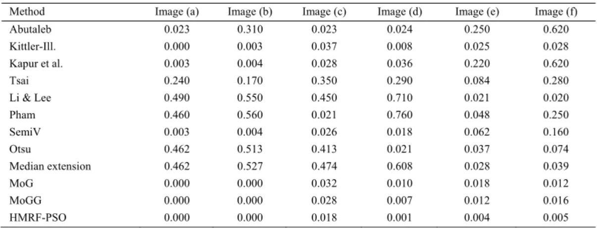
5. E In estim disti tests itera PSO I II III Fig. 2 W thres Of G this metr ME W indic grou In used meth Experimental n HMRF-PSO mator. Each p inctive parts in s conducted, ation_number= O are shown in (a)
2. (I) original ima
We performed shold-based m Generalized G purpose, we ric in the com
gives the perc
Where FO and cate foregroun und-truth regio n table 1, are d on the six N hod. l Results O combination particle displa n the image, PSO param =100 and B=1 n figure 2.I, fig (b
ages; (II) ground t
several tests methods [1] th Gaussians (MO have used N mparison. For centage of mis d BO indicate nd and backgr ons, ME is zer given the mis NDT images sh n, we have use acement is d Pij is ୲୦ mean meters have 1. Six NDT im gure 2.II and f
b)
truth images; (III
to assess perf at are: Otsu m OGG), Abutal DT images. M binary image sclassified pix % 1 ME foreground a round in the s ro. ME equals sclassification hown in figur ed PSO metho defined as: ୧ሺ n of the୲୦pa been set mages, their gr figure 2.III res
(c) I) result of segmen formance of t method, Media eb, Kittler-Ill, Misclassificat e (constituted xels, defined a 2 % 7 % 2 % F F and backgroun segmented im s one if there a n errors in the re 2.I. The res
od to minimiz ሺሻ ൌ ሺP୧ଵǡP୧ଶ article and g=< to: size=80, round truth an spectively. (d) ntation using HM the method us an extension, M , Kapur et al, ion Error ME d by a foregro as follows: 2 7 2 F F F nd of ground mage. For a pe all pixels are m e segmented im sults clearly sh ze the formula ଶǡ ǥ ǡP୧୨ǡ ǥ ǡP୧ < is the fitne c1=0.7, c2 nd the segmen (e MRF-PSO method sed in our wo Mixture Of G Li & Lee, Ph E criterion is ound and a ba d truth (or ori erfect match o misclassified. mages obtaine how the super
a (3.1) given b ୧ሻ; K is the ess function. A 2=0.8, w=0.7 nted images us e) d rk by compar aussians (MO ham, SemiV an used as the p ackground) se iginal) image, of segmented ed by the elev riority of the H by the MAP e number of After several 7, vmax=5, sing HMRF-(f) ring it to ten OG), Mixture nd Tsai. For performance egmentation, (5.1) , FT and BT classes with ven methods HMRF-PSO
6. Conclusion
We have described a method that combines Hidden Markov Random Fields and Particle Swarm Optimisation to perform segmentation. A statistical study was carried out to set the parameters of the method. Performance evaluation was conducted on NDT image dataset. Misclassification Error criterion was used as a performance metric. From the results obtained, the HMRF-PSO combination method outperforms threshold based segmentation techniques. These latter are very sensitive to noise. HMRF-PSO method demonstrates its robustness and resistance to noise.
Table 1 Misclassification errors in NDT segmented images
Method Image (a) Image (b) Image (c) Image (d) Image (e) Image (f)
Abutaleb 0.023 0.310 0.023 0.024 0.250 0.620 Kittler-Ill. 0.000 0.003 0.037 0.008 0.025 0.028 Kapur et al. 0.003 0.004 0.028 0.036 0.220 0.620 Tsai 0.240 0.170 0.350 0.290 0.084 0.280 Li & Lee 0.490 0.550 0.450 0.710 0.021 0.020 Pham 0.460 0.560 0.021 0.760 0.048 0.250 SemiV 0.003 0.004 0.026 0.018 0.062 0.160 Otsu 0.462 0.513 0.413 0.021 0.037 0.074 Median extension 0.462 0.527 0.474 0.608 0.028 0.039 MoG 0.000 0.000 0.032 0.010 0.018 0.012 MoGG 0.000 0.000 0.028 0.007 0.012 0.016 HMRF-PSO 0.000 0.000 0.018 0.001 0.004 0.005 References
[1] Beauchemin, M. (2013). Image thresholding based on semivariance. Pattern Recognition Letters, 34(5), 456-462.
[2] Dempster, A. P., Laird, N. M., & Rubin, D. B. (1977). Maximum likelihood from incomplete data via the EM algorithm. Journal of the Royal statistical Society, 39(1), 1-38.
[3] Deng, H., & Clausi, D. A. (2004). Unsupervised image segmentation using a simple MRF model with a new implementation scheme. Pattern recognition, 37(12), 2323-2335.
[4] Eberhart, R.C., & Kennedy, J. (1995). A new optimizer using particle swarm theory. In Proceedings of the sixth international symposium on micro machine and human science (Vol. 1, pp. 39-43).
[5] Eberhart, R. & Shi, Y. (2000). Comparing inertia weights and constriction factors in particle swarm optimization. In, 2000. Proceedings of the Congress on Evolutionary Computation (Vol. 1, pp. 84-88). [6] Engelbrecht, A. P. (2006). Fundamentals of computational swarm intelligence. John Wiley & Sons. [7] Geman, S., & Geman, D. (1984). Stochastic relaxation, Gibbs distributions, and the Bayesian restoration of images. IEEE Transactions on Pattern Analysis and Machine Intelligence, (6), 721-741.
[8] Gu, D. B., & Sun, J. X. (2005). EM image segmentation algorithm based on an inhomogeneous hidden MRF model. IEE Proceedings-Vision, Image and Signal Processing, 152(2), 184-190.
[9] Li, S.Z. (2001). Markov Random Field Modeling in Computer Vision. New York: Springer-Verlag. [10] Sezgin, M. (2004). Survey over image thresholding techniques and quantitative performance evaluation. Journal of Electronic imaging, 13(1), 146-168.
[11] Trelea, I.C. (2003). The particle swarm optimization algorithm: convergence analysis and parameter selection. Information processing letters, 85(6), 317-325.