Does Activating Sick-Listed Workers Work? Evidence from a
Randomized Experiment
Kai REHWALD∗ Michael ROSHOLM† Bénédicte ROULAND‡§
Work-in-progress This version: February 2014
Abstract
Reporting from a large-scale randomized controlled trial conducted in Danish job centers, this paper investigates the effects of intensified activation measures on sick-listed workers’ subsequent labor market outcomes. By exploiting variations in local treatment strategies, both between job centers and between randomly selected treatment and control groups within a given job center, we are able to compare the relative effectiveness of alternative interven-tions. Our results show that graded return-to-work programs increase the time spent in regular employment and non-benefit receipt, and reduce the time spent in unemployment. Traditional activation and preventive healthcare activation appear to have no or even adverse impacts.
JEL Classification: J68, C93, I18
Keywords: Sickness absence, Return-to-work, Active Labor Market Policies, Treatment Effects Evaluation, Randomized Controlled Trial
1
Introduction
As highlighted in the OECD report on Sickness, Disability and Work (2010), sickness policies are rapidly moving to center stage in the economic policy agenda of most OECD countries. Obviously, one of the reasons is the budgetary facet. Expenditure on paid sick leave in OECD countries amounted on average to 0.8% of GDP in 20071. Although this number might seem
∗K. Rehwald ([email protected]): Department of Economics and Business, Aarhus University
†M. Rosholm ([email protected]): Department of Economics and Business, Aarhus University
‡B. Rouland ([email protected]): Department of Economics and Business, Aarhus University.
§The paper has benefited from the comments received at the TEPP Conference “Research on health and labour”,
the 2013 DGPE workshop and the 2013 CAFÉ workshop on Labour Market Research and Impact Studies. We also want to thank the participants of the seminars given at CREST (Paris). Financial and material support by the Danish Labour Market Authority is also gratefully acknowledged. The usual disclaimer applies.
1
OECD data on social expenditure, taken from the OECD report onSickness, Disability and Work (2010).
Sickness refers to public and mandatory private paid sick leave programmes (occupational injury and other sickness daily allowances).
rather small at first sight, it is actually a matter of great concern in the current context of growing public deficits and debt burdens. In comparison, public spending on unemployment benefits reached “only” 0.55% of GDP in the same year23. Furthermore, sickness absence also implies reduced labor supply4, lost production, and health costs.
Beyond the financial aspect of paid sick leave, concerns about sick-listed workers’ reintegra-tion into the labor market are also very important. Empirical labor market research has shown that frequent and/or long-term absence spells are associated with a higher risk of unemploy-ment (Hesselius (2007)) and significantly reduce subsequent employunemploy-ment and earnings prospects (Markussen (2012)). Thus, the likelihood that a worker becomes inactive and dependent on permanent disability pension also rises.
Under these circumstances, well-wrought sickness policies are of great importance both for the individual sick-listed worker (in terms of successful reintegration) and for society as a whole (regarding public budgets). In particular, they have recently shifted from a passive towards a more employment-orientated approach, aiming both at reducing benefit dependency and increas-ing employment rates5. Taking Denmark as an example, an activation measure has been used in 16% of all sickness benefit spells in the period 2009-2011 while it amounted to 7% in the period 2005-2007 (Boll et al. (2010)). Active measures can include traditional activation programs (counseling and training) as well as preventive healthcare activation and graded return-to-work programs.
Our aim in this paper is to compare the relative effectiveness of these alternative interven-tions. Specifically, we report from a large-scale randomized controlled experiment conducted in Danish job centers in 2009 among newly registered sick-listed workers. The treatment lasted four months and consisted of a combination of weekly meetings with caseworkers and intensive acti-vation measures in the form of graded return-to-work, traditional actiacti-vation and/or preventive healthcare activation.
Our empirical strategy and key results can be summarized as follows. We first rely on a sim-ple difference in means approach to identify the causal effect of offering an intensified treatment package on newly sick-listed workers’ subsequent labor market outcomes. Specifically, we esti-mate a causalintention-to-treateffect on four outcomes variables: accumulated weeks in regular employment, self-sufficiency (i.e. all forms of non-benefit receipt), sickness and unemployment. Each of them is evaluated weekly up to three years after randomization. Second, in the spirit of Markussen and Røed (2014), we exploit variation in local treatment strategies, both between
2
OECD data on Labour Market Programmes, extracted from OECD data bank (http://stats.oecd.org/).
3As to Denmark (the country under consideration in this paper), expenditure on paid sick leave amounted to
1.4% of GDP in 2007, and public spending on unemployment benefits amounted to 0.96% of GDP.
4
According to the Danish Ministry of Employment, total sickness absence (short and long term) in 2006 reduced labor supply by 5%, which implied a cost above 2% of GDP.
5
job centers and between treatment and control groups within a given job center, to compare the relative effectiveness of the alternative measures.
Our findings reveal, first, that the experimental intervention as a whole has been ineffective. Sick-listed workers initially assigned to the treatment group spent less time in regular employ-ment and self-sufficiency compared to their peers in the control group who benefited from the normal effort. Nevertheless, our results also show that offering graded return-to-work programs more intensively is associated with an increase in regular employment and self-sufficiency, and a decrease in unemployment. Traditional activation and preventive healthcare activation, on the other hand, appear to have either no or even adverse impacts. All in all, our results thus suggest that graded return-to-work programs are the most effective intervention to improve sick-listed workers’ subsequent labor outcomes. They are associated with strong and lasting effects, but only for sick-listed workers from regular employment and for those who have physical disorders. Our study relates to the rich literature on the effectiveness of ALMPs for unemployed workers (see Card, Kluve and Weber (2010) for a meta-analysis), and particularly to the expanding literature on the impacts of workplace-based interventions for sick-listed workers (see for instance the review by van Oostrom et al. (2009)). Positive effects have been found for some groups. For instance, Markussen, Mykletun and Røed (2012) find that activation requirements in Norway bring down benefit claims and reduce the likelihood that long-term sickness absence leads to inactivity. Høgelund, Holm and McIntosh (2010) find that participation in a Danish graded return-to-work program significantly increases the probability that sick-listed workers return to regular working hours. However, Høgelund, Holm and Eplov (?) do not find any impact of graded return-to-work programs for workers with mental health problems. Andrén and Andrén (2008) find mixed effects of part-time sick leave on the probability of returning to work, with full recovery of lost work capacity (positive effect only for spells longer than 120 days).
The present essay adds to the existing literature by offering a comprehensive evaluation of intensified activation measures on sick-listed workers’ subsequent labor market outcomes. In particular, we do not focus only on workplace interventions but also on preventive healthcare activation. We do not focus either only on a specific group but consider all kind of disease. Be-sides, we provide a comparison of the relative effectiveness of alternative intensified interventions (traditional activation vs. health care preventive activation vs. graded return-to-work). It is also worth highlighting that our study is based on an experimental design, which makes our results particularly relevant.
The rest of the paper is organized as follows. Section 2 gives details about the randomized experiment. Data and variables are described in section 3. We explain our empirical strategy in section 4 and present our findings in section 5. Sensitivity and robustness analyses are provided
in section 6. Section 7 concludes.
2
The randomized experiment
Background In this study, we focus on residents in Denmark, newly sick-listed and receiving sickness benefits to replace an income loss during temporary illness (as opposed to sick-listed workers who receive a disability benefit because of a permanently reduced work capacity). In Denmark, the sickness insurance covers all employed workers, self-employed and individuals receiving unemployment insurance benefits. Sick leaves extending beyond two weeks must be sanctioned by the worker’s general practitioner, and workers have the right to receive sickness absence benefits from their municipality up to one year within a period of 18 months following the onset of an illness. The employers pay the benefits for the first 14 days of the illness period (municipalities take over afterwards).
By law, municipalities are obliged to follow-up all cases no later than in the eighth week of sickness absence and must help the sick-listed individual to return to work as quickly as possible. To promote a swift return-to-work, follow-up meetings are hold and the municipal caseworkers can apply various vocational rehabilitation measures, including coaching and retraining, job training, subsidized employment and graded return-to work6. This is the usual procedure applied to sick-listed persons.
The experiment The National Labour Market Authority in Denmark launched in early 2009 a randomized controlled trial (RCT hereafter) to test on a small scale some of the elements that will be included in a forthcoming legislation on active responses to people receiving sickness benefits7. Overall, the purpose of this experiment was to examine whether sick-listed workers
who conduct a more active role in their sickness period can achieve a greater degree of autonomy (in terms of rapid return to work and of job retention) than they would have done without the more active efforts. The present study reports from this experiment.
The experiment was designed as an RCT conducted in 16 job centers all across Denmark, with “random” assignment to treatment by birth year, even or odd. 5,652 newly sick-listed workers have been covered by the experiment, of which 2,795 persons were assigned to the control group and 2,857 people to the treatment group. Assignment to the treatment group was notified during the first follow-up meeting (no later than the eighth week of sickness absence) with a standardized
6
If the sick-listed worker, despite medical treatment and vocational rehabilitation, is unable to return to ordinary employment, the municipality may refer him or her to a permanent wage-subsidized job under special
conditions, e.g., reduced working hours and special job tasks (fleksjob). To be eligible for afleksjob, the sick-listed
worker must have a permanently reduced work capacity of at least 50%. If the sick-listed individual cannot return to afleksjob, the municipality may award a disability benefit.
7
A new and intensified treatment package was eventually rolled out nationally (with adjustments) in late 2009, when a new law governing the activation of sick-listed workers was passed in Denmark.
letter from The National Labour Market Authority.
The treatment lasted 18 weeks (four months) and consisted of a combination of weekly meetings with caseworkers AND intensive activation measures in the form of graded return-to-work, traditional activation and/or preventive healthcare activation. Newly registered sick-listed workers born in odd years received intensive efforts (treatment group), while new sick leave born in even years received normal effort (control group). Although assignment to treatment was not random but predetermined, we will treat it as an RCT; individuals were not made aware of the assignment mechanism, and birth year is “random” from the perspective of the individual.
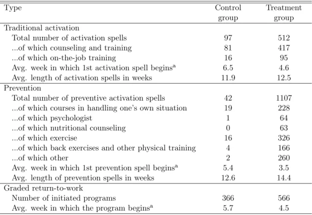
More precisely, traditional activation included vocational guidance advice and courses aimed at enhancing skills, together with internships and on-the-job training. Prevention could consist of courses in handling one’s own situation, psychological consultations, nutritional counseling, exercise as well as back exercises and other physical training. Within four weeks after the first interview, individuals in the treatment group were required to participate in some kind of activation (graded return-to-work, traditional activation and/or prevention) for at least ten hours a week in a time period of up to four months. Table 1 gives details about the extent of these activation measures. Compared to the control group, it is clear that intensive activation (in a broad sense) has been initiated for the treatment group, with a higher number of activation spells, starting earlier and lasting longer on average.
Table 1: Number of activation spells by type and treatment status
Type Control
group
Treatment group Traditional activation
Total number of activation spells 97 512
...of which counseling and training 81 417
...of which on-the-job training 16 95
Avg. week in which 1st activation spell beginsa 6.5 4.6
Avg. length of activation spells in weeks 11.9 12.5
Prevention
Total number of preventive activation spells 42 1107
...of which courses in handling one’s own situation 19 228
...of which psychologist 1 64
...of which nutritional counseling 0 63
...of which exercise 16 326
...of which back exercises and other physical training 4 166
...of which other 2 260
Avg. week in which 1st prevention spell beginsa 5.4 3.5
Avg. length of prevention spells in weeks 12.6 14.4
Graded return-to-work
Number of initiated programs 366 566
Avg. week in which the program beginsa 5.7 4.5
aMeasured in weeks since the first follow-up meeting with the municipal caseworker (which occurs eight
Moreover, the first follow-up meeting with the municipal caseworker (eight weeks after the onset of illness) could also result in total program exemption for some sick-listed workers. As shown in Table 2, around 13% of all participants in the experiment have been excused from any kind of activation measure, mainly because therapy was a hindrance (52% of all cases of exemption) and due to a pregnancy-related illness (44% of cases). However, the exempted are included in the analysis, since exemption rates were larger in the treatment group (around 17%) than in the control group (almost 10%). Specifically, the exempted from the treatment group received the treatment as usual (i.e. same as individuals in the control group) and are included in the treatment group. The exempted from the control group also received normal effort (even though they were excused). We account for this significant number of “no-shows” by estimating intention-to-treat effects, so our results can be valid even in the presence of imperfect compliance.
Table 2: Number of individuals excused/not excused by reason and treatment status
Control group Treatment group
Excused 272 496 Early retirement 7 14 Terminal illness 3 2 Pregnancy-related illness 167 174 Therapy is a hindrance 95 306 Not excused 2,523 2,361 Total 2,795 2,857
Notes: The table shows the number of individuals excused/not excused by treatment status. The exempted are included in the analysis since exemption rates were larger in the treatment group than in the control group. Specifically, the exempted from the treatment group received the treatment as usual (i.e. same as individuals in the control group) and are included in the treatment group. The exempted from the control group also received normal effort (even though they were excused).
It is worth noticing that job centers mastered the actual organization of the experiment. They carried out interviews and decided on the composition and content of activation measures that were needed, accounting for the individual’s needs and requirements and adapting to local conditions. Hence, one can suspect some variations in treatment intensities between job centers. From Figure 1, it is actually very clear that there is substantial variation in activation intensities, both between the 16 job centers covered by the experiment as well as between treatment and control groups within a given jobcenter8. As we will explain in Section 4, we exploit this variation in local treatment strategies to compare the effectiveness of the alternatives activation measures (graded return-to-work, traditional activation and prevention).
8Similarly, the overall management of the usual activation is regulated by law, but assessment and
imple-mentation of individual cases is controlled at the job center level. Hence, there was also substantial variation in activation measures among the control group.
Figure 1: Meeting and activation intensities by job center and treatment status 0 2 4 6 8 Activation intensity 1 2 3 4 5 6 7 8 9 10 11 12 13 14 15 16 0 2 4 6 8 10 Prevention intensity 1 2 3 4 5 6 7 8 9 10 11 12 13 14 15 16 0 .1 .2 .3 .4
Graded return intensity 1 2 3 4 5 6 7 8 9 10 11 12 13 14 15 16
Control group Treatment group
Notes: Indices 1 to 16 on the horizontal axes stand for job centers: Bornholm (1), Gentofte (2), Greve (3), København (4), Ringsted (5), Vordingborg (6), Ålborg (7), Morsø (8), Randers (9), Holstebro (10), Herning (11), Horsens (12), Svendborg (13), Nyborg (14), Odense (15), Åbenrå (16). Graded-return intensities are calculated as the fraction of individuals participating in a graded return program within the first 20 weeks. Activation intensities are calculated as the average number of activation weeks per individual in the first 20 weeks after the experiment began. Similarly for prevention intensities.
3
Data and variables
The empirical analysis is based on three different data sets. First, we are able to exploit unique Danish data derived from the controlled field experiment described above. In particular, the data encompass binary variables for each type of activation measure (graded return, traditional activation and prevention) and for each meeting scheduled/held, as well as the number of hours per week in each type of activation. Hence, we can follow participation accurately on a weekly basis. The data also include information about possible exemption from activation and identifies the job center.
Second, from the DREAM register, we have weekly information about the kind of social welfare benefit received as well as about individual characteristics. DREAM is constructed by gathering information from several different sources (Danish Ministries of Employment, Social Affairs, Education and Integration, as well as the 98 municipalities and Statistics Denmark). It contains a complex data structure where the type of social benefit received in a given week is represented by a unique three-digit compensation code9. This classification scheme includes all types of public income transfer schemes in Denmark. DREAM is updated once per month by the The National Labour Market Authority by adding new columns/weeks and new rows/citizens. The weekly status variables are only allowed to contain one type of compensation per week. This implies that the types of social benefits are ranked, and the ranking implies that if a citizen changes the type of social benefit in the middle of a week, only the highest ranked type is registered that week. If a citizen in a period does not receive social benefits, the period is represented by missing week-variables. From the eIncome register, we have monthly information on earnings from work. This information is used to distinguish weeks in employment from weeks where an individual is neither working nor receiving any type of transfer income.
Data on registrations in the DREAM database were obtained from the week in which the experiment began (i.e. between the first week of January 2009 and the third week of November 2009) up to the end of 2012, allowing a three years follow-up. Our four outcome variables are generated using the variablesstatus and employment encompassed in the DREAM register. Specifically, we look at the causal effect of treatment package/activation measures on regular employment, self-sufficiency with regard to public transfers, sickness and unemployment. The outcomeregular employment is defined from the status 500, i.e. is equaled to one if the latter is equaled to one (and zero otherwise). Self-sufficiency is equaled to one if the variableemployment
is equaled to one (and zero otherwise). The sickness indicator is based on the statuses 890 to 899 (i.e. equaled to one if one of these statuses is equaled to one, zero otherwise). As to the
9For instance, the code ’111’ stands for “full insured unemployment”, ’112’ for “insured unemployment (>50
percent of the week)”. The code ’890’ reflects “sickness benefits, passive” while ’899’ corresponds to “sickness benefits, graded return”.
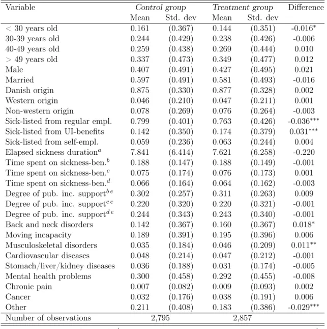
unemployment indicator, it is generated from the statuses 111, 112, 124, 125, 130 to 138, 200 to 300, and 730 to 738 (also equaled to one if one of these statuses is equaled to one, zero otherwise). Besides the treatment package, our explanatory variables include age, gender, marital status, country of origin (three categories - Denmark, western countries and non-western countries), the state occupied before sickness (three categories - job, UI benefits and self-sufficiency), the elapsed sickness duration at the start of the experiment, the fraction of time spent on sickness payments (in the year before sickness, in the second last year before sickness and in the third last year before sickness), and the same fraction for time spent on public income support of any kind (also in the first, second and third year before sickness). Table 3, which shows means and standard deviations of the explanatory variables by treatment status, suggests that there are very few observed differences between treatment and control groups10. “Random” assignment based on the birth year - even or odd - has been successful in balancing groups. The most significant difference, nonetheless low, relates to the status before sickness: the treatment group has been on average a bit less in regular employment than the control group (76.3% against 79.9%), and a bit more in unemployment (17.4% against 14.2% on average).
Finally, from Statistics Denmark, we have data on socio-economic characteristics at the municipality level. In particular, for each municipality, we are able to collect annual data on the total fertility rate, average age, life expectancy for new born babies, as well as the share of the labor force on full-time unemployment (quarterly information). Furthermore, we can calculate quarterly ratios of the working-age population outside the labor force and of the highest attained education level of the working-age population to the 15-69 years old population. We use this information to control for local environment characteristics when exploiting the variation in treatment strategies across job centers.
4
Estimation strategies
4.1 Difference in means approach
We first aim at identifying the causal effect of offering the intensified treatment package, as a whole, on newly sick-listed workers’ subsequent labor market outcomes. In order to do so, we estimate the following model:
Yi =β0+βZZi+Xiβ+εi (1)
whereYi is the outcome of individuali(we consider four alternative measures evaluated at dif-10
Table 10 in appendix gives means and standard deviations of the explanatory variables by treatment status for the sample of 4728 individuals (see further).
Table 3: Pre-treatment characteristics by treatment status
Variable Control group Treatment group Difference
Mean Std. dev Mean Std. dev
< 30 years old 0.161 (0.367) 0.144 (0.351) -0.016∗ 30-39 years old 0.244 (0.429) 0.238 (0.426) -0.006 40-49 years old 0.259 (0.438) 0.269 (0.444) 0.010 > 49 years old 0.337 (0.473) 0.349 (0.477) 0.012 Male 0.407 (0.491) 0.427 (0.495) 0.021 Married 0.597 (0.491) 0.581 (0.493) -0.016 Danish origin 0.875 (0.330) 0.877 (0.328) 0.002 Western origin 0.046 (0.210) 0.047 (0.211) 0.001 Non-western origin 0.078 (0.269) 0.076 (0.264) -0.003
Sick-listed from regular empl. 0.799 (0.401) 0.763 (0.426) -0.036∗∗∗ Sick-listed from UI-benefits 0.142 (0.350) 0.174 (0.379) 0.031∗∗∗
Sick-listed from self-empl. 0.059 (0.236) 0.063 (0.244) 0.004
Elapsed sickness durationa 7.841 (6.414) 7.621 (6.258) -0.220
Time spent on sickness-ben.b 0.188 (0.147) 0.188 (0.149) -0.001 Time spent on sickness-ben.c 0.075 (0.174) 0.076 (0.173) 0.001 Time spent on sickness-ben.d 0.066 (0.164) 0.064 (0.162) -0.003
Degree of pub. inc. supportb e 0.302 (0.257) 0.311 (0.263) 0.009 Degree of pub. inc. supportc e 0.220 (0.320) 0.220 (0.321) -0.001 Degree of pub. inc. supportd e 0.244 (0.343) 0.243 (0.340) -0.001
Back and neck disorders 0.142 (0.367) 0.160 (0.367) 0.018∗
Moving incapacity 0.189 (0.391) 0.195 (0.396) 0.006
Musculoskeletal disorders 0.035 (0.184) 0.046 (0.209) 0.011∗∗
Cardiovascular diseases 0.048 (0.214) 0.047 (0.212) -0.001
Stomach/liver/kidney diseases 0.036 (0.188) 0.031 (0.174) -0.005
Mental health problems 0.300 (0.458) 0.292 (0.455) -0.008
Chronic pain 0.007 (0.082) 0.009 (0.093) 0.002
Cancer 0.032 (0.176) 0.038 (0.191) 0.006
Other 0.211 (0.408) 0.183 (0.386) -0.029∗∗∗
Number of observations 2,795 2,857
a
at start of experiment (in weeks) bin year before sickness cin second last year before sickness din
third last year before sickness eany kind of public income support. Significance levels:∗: 10% ∗∗: 5%
ferent points in time, see below), Zi is a treatment status indicator equal to unity for clients
assigned to the treatment group (0 otherwise), andXiis the vector of pre-treatment
characteris-tics described in Table 3 (with age entering in a univariate manner). Since treatment assignment is essentially random, Zi will, by design, be independent of Xi and of any other (observed or
unobserved) pre-treatment variable. It follows immediately that conditioning onXi should leave
the parameter estimate ofβZ,βbOLSZ , unaffected. At the same time, we would expect a reduction
in the residual variance to be accompanied by an increase in precision. This is why the vector Xi is included in equation (1).
Now, note that the coefficientβZcorresponds to the difference in means of outcome variableYi
between treatment and control group. It identifies the intention-to-treat (ITT) effectE(Yi|Zi = 1)−E(Yi|Zi= 0)if E(εi|Zi) =E(εi). This is likely to hold given thatZi is assigned at random
(cf. above). The OLS estimator of βZ, the experimental impact estimate βbZOLS, can be given a
causal interpretation. It is unbiased and consistent.
Regarding the dependent variable in equation (1),Yi, we consider four measures: accumulated
weeks - running sums counting from week one after the start of the experiment - in regular employment, self-sufficiency, sickness and unemployment (each of them evaluated weekly up to three years after randomization). All individuals can be followed for 141 weeks, and outcome variables examined three years (156 weeks) after enrolment are non-missing for all but eight individuals. The self-sufficiency measure is meant to cover all forms of non-benefit receipt. It encompasses individuals in regular (i.e. wage) employment, as well as self-employed, housewives and everybody else not receiving public income transfers11.
Besides its ease - interpreting and communicating the results is straightforward - the main advantage of the identification strategy discussed above is that results are valid even in the presence of imperfect compliance. Recall that there is a significant number of “no-shows”; more than one out of six sick-listed workers initially assigned to the treatment group were excused from treatment (see Table 2) and received treatment as usual. Furthermore, the ITT approach scores high from a policy analysis and design perspective. In fact, one of the aims of the experiment was to test the new and intensified treatment package on a small scale (impact pilot) before it was eventually rolled out nationally (with adjustments) in 2009 when a new law governing the activation of sick-listed workers was passed in Denmark. The main drawback, however, is that the simple “difference in means approach” only allows us to evaluate the combined treatment package as a whole. Nothing can be said about the relative effectiveness of alternative interventions (traditional activation vs. preventive healthcare activation vs. graded return-to-work). Our second identification strategy, which is in spirit of the one used by Markussen and Røed (2014),
11
Exceptions are (subsidized) adult apprentices (“Voksenlærlinge”) and individuals receiving state educational support (“Statens Uddannelsesstøtte”). Both groups are considered to be “self-sufficient”.
aims to overcome this limitation.
4.2 Local treatment strategies approach
By exploiting variations in local treatment strategies, Markussen and Røed (2014) analyze the effectiveness of four alternative vocational rehabilitation programs for a large sample of temporary disability benefit recipients in Norway. We will follow their approach without technical changes. To begin with, recall that there is substantial variation in treatment intensities both between the 16 jobcenters covered by the experiment and between treatment and control group within a given jobcenter. As such, there are 32 separate “local treatment environments” which are characterized by idiosyncratic working methods and treatment priorities. Differences in these “treatment cultures” may manifest themselves, e.g., in the choice and combination of treatment types, in the speed by which newly registered clients are exposed to them, or in the length of initiated activation spells. The resulting “treatment portfolio” is shaped by each of these choices, which may, in sum, be referred to as a “treatment strategy”. Our aim is to proxy these treatment strategies by vectors of local treatment strategy characteristics (φi). These can, in turn, be used
to identify the effects of alternative interventions.
The vectors of local treatment strategy characteristics (φi) are individual-specific and depend
on the treatment histories of all other sick-listed workers exposed to the same local treatment regime (more on this below). Each vector contains three elements -φSi(S=traditional activation,
preventive healthcare activation, graded return-to-work) - and is meant to describe “both the choice of (first) treatment, and the speed by which it is implemented” (Markussen and Røed (2014)).
Following Markussen and Røed (2014), we estimate the vector of local treatment strategy characteristics in the framework of a linear discrete transition rate model with competing risks. In particular, we consider exits from a single state (“sick and untreated”) to multiple destinations: participation either in traditional activation, in preventive healthcare activation, or in a graded return-to-work program. Albeit a sick-listed individual can be exposed to a combination of alternative interventions over the course of his sickness career (cf. above), destinations are mutually exclusive in the sense that a person can only participate in one program at a time. Moreover, our focus lies on the choice of the first treatment. Accordingly, the data pattern used for estimation is characterized by single spells, one for each individual; repeat spells are ignored. The survival time data at hand is an interval censored inflow sample with weekly observations. Now, letPSijd be a destination-specific censoring variable equal to unity (zero otherwise) if
sick-listed individuali, registered in local treatment environmentj makes a transition into treatment
S after having been untreated - and thus at risk of making the transition - for dweeks. Given these mutually exclusive event indicators, we organize the dataset in the following way. Starting
with a panel in person-week format, we remove, for each sick-listed worker, observations after the first transition into one of the three alternative programs. Uncompleted spells are right-censored in the absence of an event within the first 20 weeks - recall that the treatment period is meant to last only 18 weeks and note that there are virtually no treatment incidences after the 20th week - or if the sickness spell ends. In short, the resulting panel is unbalanced and contains, for each individual, one observation per week at risk of being activated for the first time.
Then, lettingD denote a vector of duration dummies (one for each week), Xi the vector of
individual-specific pre-treatment characteristics described in Table 10 in Appendix (where age and the elapsed sickness duration at the start of the experiment enter non-parametrically) and Xjda vector of municipality-level socio-economic characteristics of local treatment environment
j in week d after randomization (unemployment rate, labor force participation, a measure of educational attainments, total fertility rate and quadrics of mean age and life expectancy), we estimate - separately for each of the three alternative treatments - the following linear probability model:
PSijd=β0+DλS+XiθS+XjdϑS+uSijd (2)
Markussen and Røed (2014) argue that the residuals in this model have an appealing inter-pretation. Particularly, the sum of individual residuals,
b uSij = DSi ∑ d=1 b uSijd (3)
where DSi corresponds to the number of weeks sick-listed worker i was at risk of making the
transition into treatment S, can “be interpreted as the estimated covariate-adjusted transition propensity at the claimant level”. Right-censoring and duration dependence aside,ubSij is equal to
the (weighted) number of “lacked” waiting weeks for transition intoScompared to what one would expect given the observed pre-treatment characteristics of clienti(Xi) and the municipality-level
socio-economic characteristics of local treatment environment j (Xjd). For instance, ubSij > 0
indicates that the transition happened earlier than expected (Markussen and Røed (2014)). Now, recall that the vector of local treatment strategy characteristics is meant to describe both the choice of the first treatment and the speed by which newly registered clients are exposed to it. Specifically, the elements (φSi) of the vector of local treatment strategy characteristics
relevant for individual i may be defined as the average value of buSij of all sick-listed workers
(other than i) subject to the same local treatment regime:
φSi=
ΣiεNjubSij−buSij
Nj−1
whereNj −1 is the number of individuali’s peers in local treatment environmentj.
Equipped with the proxies of the local treatment strategy characteristics, we specify the following outcome equation:
Yi=β0+φiα+Xiγ+Xjω+εi (5)
whereYi is the outcome of individuali(we consider the same measures as in (1)),Xi andXj are
the same individual and municipality-level socio-economic characteristics as in (2) and φi is the
vector of local treatment strategy characteristics with elements φSi (S=traditional activation,
healthcare preventive activation, graded return-to-work) as defined in (4). The coefficients α
identify the impacts of marginal changes in local treatment strategies on subsequent labor market outcomes and can thus be interpreted as intention-to-treat effects.
Following Markussen and Røed (2014), “we also estimate an instrumental variables model where we use observed program participation directly as explanatory variables, and instrument them with the vector of local program intensity indicators” (φi). For this purpose, we consider
the following specification:
Yi =λ0+Piµ+Xiδ+Xjζ+εi (6)
where Pi is a vector whose elements PSi (S=traditional activation, preventive healthcare
ac-tivation, graded return-to-work) are indicators of actual treatment receipt. In particular, let
PSi equal unity (zero otherwise) if individual i participated in treatment activity S at some
time during the first 20 weeks after enrolment. A potential problem with (6) is that individuals may, at least in part, self-select into treatments of certain types, rendering Pi endogenous if
selection is based on unobservables. Consequently, we instrument the elements of the vector of actual treatment receipt indicators (PSi) by the elements of the vector of local treatment
strat-egy characteristics (φSi). These are, arguably, strong and valid instruments, for the elements of φi are, by construction, firstly, exogenous to individual i, and secondly, highly correlated with
the endogenous regressors PSi. The coefficients µidentify the impacts of actually participating
in alternative treatment activities and can, as pointed out by Markussen and Røed (2014), be interpreted as local average treatment effects (LATE).
5
Results
5.1 From the difference in means approach
To begin with, we present the results of evaluating the combined treatment package as a whole by comparing - for each of four alternative outcome variables - the difference in means between
individuals initially assigned to treatment and control group at different points in time after the start of the experiment. Does offering intensified services to newly registered sick-listed workers improve their labor market prospects relative to clients receiving treatment as usual? The answer is given in Figure 2. The considered labor market outcomes are the accumulated number of weeks spent in regular employment (upper left panel), self-sufficiency (upper right panel), sickness (lower left panel) and unemployment (lower right panel). Each figure is based on 156 separate regressions, one for each week, of the outcome measure on a treatment status indicator and a vector of background characteristics (cf. above). Confidence intervals at the 95% level (dotted lines) - based on robust standard errors - are reported along with the experimental impact estimates βbOLS
Z (solid lines).
Figure 2: Intention-to-treat effects for four alternative outcome measures at different points in time after randomization
−7 −6 −5 −4 −3 −2 −1 0 1
Weeks in reg. employment
0 52 104 156
Weeks since start of experiment
−7 −6 −5 −4 −3 −2 −1 0 1 Weeks in self−sufficiency 0 52 104 156
Weeks since start of experiment
−2 −1 0 1 2 3 Weeks in sickness 0 52 104 156
Weeks since start of experiment
−2 −1 0 1 2 3 Weeks in unemployment 0 52 104 156
Weeks since start of experiment
Intention−to−treat effect 95% confidence interval
Notes: Each figure is based on 156 separate OLS regressions (one for each week) of the accumulated number of weeks in regular (i.e. wage) employment/self-sufficiency/sickness/unemployment - running sums counting from week one after the start of the experiment - on a treatment status dummy and the vector of pre-treatment char-acteristics shown in Table 3. The solid lines show how the estimated effects of offering the intensified treatment package to newly registered sick-listed workers (the assigned treatment status parameter estimates) evolve over time. The plotted ITT effects corresponds to the difference in the average number of weeks spent in regular employment/self-sufficiency/sickness/unemployment between treatment and control group (controlling for back-ground characteristics) evaluated at a given point in time after randomization as indicated on the horizontal axis. The dotted lines depict the corresponding pointwise confidence intervals (using the robust standard errors of the estimated treatment status coefficients for each week) at the 95% level. The number of observations each regression is based on varies between 5652 for all weeks up to and including the 141st week after the start of the experiment (no missings) and 5644 for the 156th week (when eight individuals had to be excluded because their labor market status in this or in an earlier week cannot be observed).
ineffective. Offering the combined treatment package - consisting of a combination of intensi-fied activation, prevention and graded return-to-work activities - to newly registered sick-listed workers seems to have either no or even adverse impacts on subsequent labor market prospects when evaluated against the counterfactual outcomes of individuals receiving treatment as usual. Regarding the outcome variables regular employment and self-sufficiency, estimated ITT effects are negative, moderate in size and statistically significant at the 5% level in the long-run. The estimates - which can be interpreted causally (cf. above) - suggest, e.g., that offering intensified instead of standard services reduces the time spent in self-sufficiency (non-benefit receipt) by almost an entire month (3.2 weeks) on average within a time period of three years. The corresponding point estimate for the time spent in regular employment (-2.4 weeks after three years) is slightly smaller in absolute terms and borderline significant (p-value: 0.087). The two lower panels of Figure 2 show the results for the outcome measures “accumulated number of weeks in sickness” and “accumulated number of weeks in unemployment”. The observed pattern is similar for both; estimated ITT effects are positive, small in size and not statistically significant at conventional levels over the entire domain. Hence, offering the combination of intensified treatments instead of standard services appears to have, altogether and on average, no discernible effect on sickness and unemployment.
Figure 3 plots results for two alternatives outcomes, namely early retirement and “fleksjob”. Offering intensified instead of standard services significantly increases the time spent in early retirement by 2.6 weeks (p-value: 0.001) on average within a time period of three years, as well as the time spent in “fleksjob” (+1.5 week after three years, p-value: 0.051).
To conclude, the intensified treatment package as a whole comes off badly when compared to treatment as usual. While sick-listed workers initially assigned to the treatment group spent less time in regular employment and self-sufficiency compared to their peers in the control group, they spend more time in early retirement and “fleksjob”. While these effects are moderate in size and statistically significant, the impacts on sickness and unemployment are rather small and cannot be distinguished from zero.
5.2 From the local treatment strategies approach
As to the results from the “local treatment strategy approach”, have a look at Tables 4 and 5. Table 4 (OLS) reports estimates of average intention-to-treat effects of marginal changes in local treatment strategies. Estimated impacts of actually participating in alternative treatment activities (LATE) are shown in Table 5 (IV/2SLS). Following Markussen and Røed (2014), we have normalized the vectors of local treatment strategy characteristics by scaling its elementsφSi
by the inverse of the absolute difference in the average value ofφSi between the local treatment
Figure 3: Intention-to-treat effects for two alternative outcome measures at different points in time after randomization
−1 0 1 2 3 4 5
Weeks in early retirement
0 52 104 156
Weeks since start of experiment
−1 0 1 2 3 4 5 Weeks in fleksjob 0 52 104 156
Weeks since start of experiment
Intention−to−treat effect 95% confidence interval
Notes: Each figure is based on 156 separate OLS regressions (one for each week) of the accumulated number of weeks in early retirement/“fleksjob” running sums counting from week one after the start of the experiment -on a treatment status dummy and the vector of pre-treatment characteristics shown in Table 3. The solid lines show how the estimated effects of offering the intensified treatment package to newly registered sick-listed workers (the assigned treatment status parameter estimates) evolve over time. The plotted ITT effects corresponds to the difference in the average number of weeks spent in early retirement/“fleksjob” between treatment and control group (controlling for background characteristics) evaluated at a given point in time after randomization as indicated on the horizontal axis. The dotted lines depict the corresponding pointwise confidence intervals (using the robust standard errors of the estimated treatment status coefficients for each week) at the 95% level. The number of observations each regression is based on varies between 5652 for all weeks up to and including the 141st week after the start of the experiment (no missings) and 5644 for the 156th week (when eight individuals had to be excluded because their labor market status in this or in an earlier week cannot be observed). The outcomes variables are
generated using the variablestatusfrom the DREAM database. Based on the version 28th of the DREAM codes,
the outcome early retirement is defined from the statuses 621, 781, 782 and 783 (i.e. equaled to one if one of
these statuses is equaled to one, zero otherwise), and the outcome“fleksjob”is generated using the statuses 622,
difference corresponds to the difference described above and parameter estimates in Table 4 can be interpreted as the expected change in the outcome variable “resulting from a movement from the treatment environment giving lowest priority to the strategy under consideration to the one giving it highest priority”.
The OLS estimates in Table 4 suggest that prioritizing graded return-to-work programs has favorable effects. While the results indicate that offering graded return-to-work programs more intensively does not decrease the incidence of sickness in the long-run (the effect appears to be rather short-lived), they do show that graded return reduces the likelihood that sickness spells are followed by unemployment and increases the prospects of regular employment and other forms of self-sufficiency. The estimates suggest, e.g., that a movement from the treatment regime prioritizing graded return-to-work programs the least to the one giving it highest priority leads to an expected increase in the time spent in regular employment of about four months (18 weeks) within a time period of three years. The impacts on regular employment, self-sufficiency, and unemployment accumulate over time in a sustained manner and are highly statistically significant.
In short, offering graded return-to-work programs more intensively is associated with an increase in regular employment and self-sufficiency, and a decrease in unemployment. Traditional activation and preventive healthcare activation, on the other hand, appear to have either no or even adverse impacts. These findings are supported by the instrumental variable estimates reported in Table 5.
The table shows estimated effects of actually participating in one of the alternative treat-ment activities. It therefore comes as no surprise that estimates (LATE) tend to be larger in absolute terms compared to those reported in Table 4 (ITT). The estimates in Table 5 may be briefly summarized as follows. First, neither traditional activation nor preventive healthcare activation seems to have a discernible effect on subsequent labor market outcomes. None of the corresponding estimates is statistically significant at conventional levels. And second, letting sick-listed workers participate in graded return-to-work programs proves to be a very successful strategy. Participation in these programs increases the time spent in regular employment and non-benefit receipt. At the same time, it reduces the time spent in unemployment. Estimates are favorable, large in absolute size and statistically significant either at the five or even at the one percent level.
6
Robustness and sensitivity
To be completedTable 4: Estimated intention-to-treat effects of marginal changes in local treatment strategies for four alternative outcome measures at different points in time after randomization (OLS)
I II III IV
Regular employment
Self-sufficiency Sickness Unemployment
Panel A: One year after randomization (N=4728)
φactivation -1.602 -0.633 -1.042 1.393 (1.548) (1.575) (1.625) (0.959) φprevention -1.195 -1.727∗ 1.838∗ 0.065 (0.940) (0.957) (0.987) (0.582) φgradedreturn 7.232∗∗∗ 5.344∗∗∗ -3.870∗∗ -0.755 (1.816) (1.849) (1.907) (1.125)
Panel B: Two years after randomization (N=4728)
φactivation -5.174∗ -3.689 -1.179 2.454 (3.126) (3.142) (2.555) (1.998) φprevention -3.180∗ -4.415∗∗ 1.762 1.542 (1.911) (1.920) (1.562) (1.221) φgradedreturn 13.793∗∗∗ 9.805∗∗∗ -2.618 -5.693∗∗ (3.713) (3.731) (3.035) (2.373)
Panel C: Three years after randomization (N=4720)
φactivation -5.233 -3.064 -2.617 1.347 (4.620) (4.620) (2.949) (2.933) φprevention -3.786 -5.105∗ 0.434 2.054 (2.852) (2.852) (1.821) (1.811) φgradedreturn 18.496∗∗∗ 15.318∗∗∗ -0.915 -9.528∗∗∗ (5.662) (5.662) (3.614) (3.594)
Notes: The table shows estimated intention-to-treat effects of marginal changes in local treatment strate-gies. Each panel (A/B/C) is based on four separate OLS regressions of the accumulated number of weeks in regular (i.e. wage) employment/self-sufficiency/sickness/unemployment - running sums counting from week one after the start of the experiment - on the normalized vector of local treatment strategy character-istics and additional controls (individual and municipality-level socio-economic charactercharacter-istics). Outcome variables in panel A/B/C are evaluated one/two/three years after randomization. The number of obser-vations (N) amounts to 4728 in panels A and B, and to 4720 in panel C (for which eight individuals had to be excluded because their labor market status three years after randomization cannot be observed).
Table 5: Estimated effects of participating in alternative treatment activities (LATE) for four alternative outcome measures at different points in time after randomization (IV/2SLS)
I II III IV Regular employment Self-sufficiency Sickness Unemployment
Panel A: One year after randomization (N=4728)
Activation 3.699 3.636 -5.484 1.758 (4.314) (3.529) (3.467) (2.143) Prevention 3.597 0.895 -0.335 0.826 (3.930) (3.203) (3.150) (1.949) Graded return-to-work 46.893∗∗ 26.013∗ -10.194 -14.080 (19.230) (14.701) (14.714) (9.233)
Panel B: Two years after randomization (N=4728)
Activation -7.152 -3.258 -4.342 3.957 (6.550) (5.954) (4.919) (4.164) Prevention -3.642 -7.274 1.927 3.120 (6.358) (5.796) (4.783) (4.057) Graded return-to-work 59.924∗∗∗ 29.541 0.928 -32.892∗∗ (23.040) (20.156) (16.842) (13.978)
Panel C: Three years after randomization (N=4720)
Activation -5.755 -0.328 -6.767 1.382 (9.908) (9.311) (5.328) (6.061) Prevention 3.332 0.061 -5.099 2.318 (9.846) (9.238) (5.315) (6.061) Graded return-to-work 118.070∗∗∗ 97.137∗∗ -4.004 -61.625∗∗ (42.438) (42.182) (22.822) (26.748)
Notes: The table shows estimated effects of participating in alternative treatment activities (local average treatment effects). Each panel (A/B/C) is based on four separate IV/2SLS regressions (second stage). See notes to Table 4 for a description of the outcome variables and additional controls. Outcome variables in panel A/B/C are evaluated one/two/three years after randomization. The number of observations (N) amounts to 4728 in panels A and B, and to 4720 in panel C (for which eight individuals had to be excluded because their labor market status three years after randomization cannot be observed). Standard errors
Table 6 (results for the control group only)
Table 7 (results accounting only for the variation in treatment intensities between treatment and control groups)
Table 8 (by labor market status before sickness) Table 9 (by illness type)
Table 6: Estimated effects of participating in alternative treatment activities - control group only
I II III IV Regular employment Self-sufficiency Sickness Unemployment
Panel A: One year after randomization (N=2304)
Activation 24.894 -6.286 -43.142 42.701 (42.247) (47.374) (44.728) (28.424) Prevention 57.686 34.909 -17.251 -2.587 (43.972) (43.725) (47.288) (29.548) Graded return-to-work 0.706 -23.702 10.867 7.218 (17.474) (17.884) (18.653) (11.736)
Panel B: Two years after randomization (N=2304)
Activation -207.005 -224.058 143.523 -19.931 (125.903) (139.647) (101.665) (66.048) Prevention 62.589 33.857 73.798 -111.906∗ (122.202) (147.135) (97.014) (67.458) Graded return-to-work -2.437 -43.613 32.491 -5.086 (34.490) (37.791) (27.773) (18.072)
Panel C: Three years after randomization (N=2297)
Activation -125.678 -218.556 133.977 -59.748 (159.319) (186.218) (122.996) (114.910) Prevention 71.137 -69.209 157.585 -144.519 (199.180) (231.319) (138.877) (148.031) Graded return-to-work 17.728 -14.324 22.501 -7.740 (32.327) (37.165) (26.695) (23.254)
Notes: The table shows estimated effects of participating in alternative treatment activities (local average treatment effects) for the control group. Each panel (A/B/C) is based on four separate IV/2SLS regressions (second stage). See notes to Table 4 for a description of the outcome variables and additional controls. Outcome variables in panel A/B/C are evaluated one/two/three years after randomization. The number of observations (N) amounts to 2304 in panels A and B, and to 2297 in panel C (for which seven individuals had to be excluded because their labor market status three years after randomization cannot be observed).
Standard errors in parentheses. Significance levels: ∗: 10%
7
Conclusion
This paper provides new important evidence on the effects of intensified activation measures on sick-listed workers’ subsequent labor market outcomes. We use a unique dataset from a large-scaled randomized experiment conducted in Danish job centers in 2009, linked to large
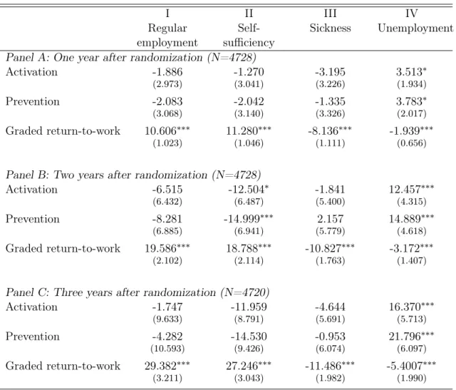
Table 7: Estimated effects of participating in alternative treatment activities - accounting only for variation between groups (treatment/control)
I II III IV Regular employment Self-sufficiency Sickness Unemployment
Panel A: One year after randomization (N=4728)
Activation -1.886 -1.270 -3.195 3.513∗ (2.973) (3.041) (3.226) (1.934) Prevention -2.083 -2.042 -1.335 3.783∗ (3.068) (3.140) (3.326) (2.017) Graded return-to-work 10.606∗∗∗ 11.280∗∗∗ -8.136∗∗∗ -1.939∗∗∗ (1.023) (1.046) (1.111) (0.656)
Panel B: Two years after randomization (N=4728)
Activation -6.515 -12.504∗ -1.841 12.457∗∗∗ (6.432) (6.487) (5.400) (4.315) Prevention -8.281 -14.999∗∗∗ 2.157 14.889∗∗∗ (6.885) (6.941) (5.779) (4.618) Graded return-to-work 19.586∗∗∗ 18.788∗∗∗ -10.827∗∗∗ -3.172∗∗∗ (2.102) (2.114) (1.763) (1.407)
Panel C: Three years after randomization (N=4720)
Activation -1.747 -11.959 -4.644 16.370∗∗∗ (9.633) (8.791) (5.691) (5.713) Prevention -4.282 -14.530 -0.953 21.796∗∗∗ (10.593) (9.426) (6.074) (6.097) Graded return-to-work 29.382∗∗∗ 27.246∗∗∗ -11.486∗∗∗ -5.4007∗∗∗ (3.211) (3.043) (1.982) (1.990)
Notes: The table shows estimated effects of participating in alternative treatment activities (local average treatment effects), accounting only for the variation in treatment intensities between treatment and control groups (i.e two local treatment strategies, instead of 32). Each panel (A/B/C) is based on four separate
IV/2SLS regressions (second stage). See notes to Table 4 for a description of the outcome variables
and additional controls. Outcome variables in panel A/B/C are evaluated one/two/three years after
randomization. The number of observations (N) amounts to 4728 in panels A and B, and to 4720 in panel C (for which eight individuals had to be excluded because their labor market status three years after
randomization cannot be observed). Standard errors in parentheses. Significance levels: ∗: 10% ∗∗: 5%
Table 8: Estimated effects of participating in alternative treatment activities, by labor market status before sickness (employment/UI-benefits recipient)
I II III IV
Regular employment
Self-sufficiency Sickness Unemployment
Panel A: One year after randomization Employment before sickness (N=3593)
Activation 2.67(4.79) 3.64 (4.44) -7.44∗ (4.33) 2.63(2.16)
Prevention 1.80(4.30) -0.08 (3.99) 0.31 (3.89) 0.32(1.94)
Graded RTWa 36.67∗∗ (14.95) 27.96∗∗ (14.24) -21.35 (13.20) -7.30 (6.69)
UI-benefits before sickness (N=838)
Activation -5.11 (8.84) -5.34 (10.47) 1.86(14.06) -0.56 (12.29) Prevention -3.81 (7.00) -4.93(8.15) -6.98 (10.72) 8.62(8.80) Graded RTWa -71.32 (102.80) -87.60 (123.55) -112.40(168.49) -87.22(153.45)
Panel B: Two years after randomization Employment before sickness (N=3593)
Activation -12.75 (9.00) -9.51 (8.42) -1.87(6.37) 2.96(4.71) Prevention -13.42 (8.82) -17.74∗∗(8.26) 8.71 (6.27) 0.75(4.63) Graded RTWa 66.30∗∗∗ (23.22) 55.94∗∗∗ (21.06) -26.96∗ (16.08) -16.56 (12.65)
UI-benefits before sickness (N=838)
Activation 7.31(13.10) 2.71(11.54) -9.89 (15.33) 2.14(12.36) Prevention 6.27(13.82) -1.80 (12.25) -29.56∗ (16.26) 20.49(13.00) Graded RTWa 152.37(204.70) -33.98 (178.99) -136.33(236.86) 14.67 (195.89)
Panel C: Three years after randomization (N=3588) Employment before sickness (N=3588)
Activation -12.37 (12.45) -4.92 (12.06) -6.22(6.66) 0.87(6.32) Prevention -6.76 (12.37) -11.67 (12.10) -1.06(6.61) -0.17 (6.32) Graded RTWa 109.9∗∗∗ (39.1) 102.0∗∗∗ (37.5) -25.38 (21.29) -32.29 (20.39)
UI-benefits before sickness (N=835)
Activation 5.60(20.73) -2.70 (24.32) -8.22 (18.03) -7.04 (18.17) Prevention 23.05 (24.10) -1.21 (28.15) -40.94∗ (27.93) 22.32(20.95) Graded RTWa -28.34 (379.14) -290.48(415.10) -104.14(305.49) 17.86 (315.44)
Notes: The table shows estimated effects of participating in alternative treatment activities (local average treatment effects), decomposing by labor market status before sickness. Estimates for employed workers and UI-benefits recipients are reported, while results for self-employed are not. There are 296 self-employed in our sample; none of the corresponding estimates is significant at conventional levels. Each panel (A/B/C) is based on four separate IV/2SLS regressions (second stage). See notes to Table 4 for a description of
the outcome variables and additional controls. Standard errors in parentheses. aGraded return-to-work.
Table 9: Estimated effects of participating in alternative treatment activities, by illness type (mental/non-mental health problems)
I II III IV
Regular employment
Self-sufficiency Sickness Unemployment
Panel A: One year after randomization (N=1544), mental health problems
Activation 3.68(5.61) 7.78 (6.69) -13.88∗ (7.93) 3.66(4.40)
Prevention 0.07(4.23) 0.01 (5.12) -2.59(6.22) 3.98(3.34)
Graded RTWa 20.60 (30.49) 28.66(41.19) -12.56 (54.54) -19.16 (25.92)
Panel A: One year after randomization (N=3184), non-mental health problems
Activation 1.15(5.75) -1.24(4.69) 1.58 (4.80) -0.83 (3.42)
Prevention 4.16(6.00) -0.92(4.87) 3.01 (4.88) -2.36 (3.25)
Graded RTWa 40.56 (25.35) 15.96(19.80) -0.52 (21.36) -18.25 (18.52)
Panel B: Two years after randomization (N=1544), mental health problems
Activation 6.10 (14.10) 13.91(15.93) -25.67∗∗∗ (9.22) 10.65 (9.67) Prevention -8.48 (11.94) -11.23 (13.30) -4.90(7.76) 13.56∗ (8.02) Graded RTWa -68.10 (66.19) -89.11 (65.14) -10.12 (40.05) 45.38(42.58)
Panel B: Two years after randomization (N=3184), non-mental health problems
Activation -11.86 (8.92) -12.31 (7.81) 6.72 (6.09) 0.10(5.43) Prevention -1.08 (10.10) -9.24(8.76) 6.30 (6.88) -2.06 (6.14) Graded RTWa 77.94∗∗ (33.38) 43.97(31.17) 8.46(23.44) -42.32∗∗ (20.60)
Panel C: Three years after randomization (N=1539), mental health problems
Activation 6.46 (19.12) 12.98(17.71) -20.67 (15.79) 9.84(11.10) Prevention 3.40(14.12) -5.01 (13.08) -9.31 (13.09) 8.92(8.21) Graded RTWa 142.28(123.70) 119.72 (112.16) -116.97(116.37) -47.24 (74.22)
Panel C: Three years after randomization (N=3181), non-mental health problems
Activation -12.35 (14.54) -9.23 (13.40) 6.14 (6.73) -2.53 (8.30) Prevention 11.39 (17.41) 8.20(16.11) -1.03(8.20) -3.26 (10.03) Graded RTWa 151.29∗∗ (65.6) 127.88∗ (63.17) -2.94 (31.60) -76.56∗ (40.61)
Notes: The table shows estimated effects of participating in alternative treatment activities (local average treatment effects), decomposing by illness type. Mental health problems cover disorders such as stress, depression. Each panel (A/B/C) is based on four separate IV/2SLS regressions (second stage). See notes to Table 4 for a description of the outcome variables and additional controls. Standard errors in parentheses.
administrative registers.
We first evaluate theintention-to-treateffect of the intensified activation package as a whole (weekly meetings with caseworkers combined with graded return-to-work, traditional activation and/or health care preventive activation) by comparing the difference in means between treated and control group. Second, we exploit variations in local treatment strategies, both between job centers and between treatment and control groups within a given job center - in spirit of Markussen and Røed (2014) - to compare the relative effectiveness of the alternative measures.
Our findings reveal, first, that the experimental intervention as a whole has been ineffective. Sick-listed workers initially assigned to the treatment group spent less time in regular employ-ment and self-sufficiency (i.e. all forms of non-benefit receipt) compared to their peers in the control group who benefited from the usual intervention. Nevertheless, our results also show that offering graded return-to-work programs more intensively is associated with an increase in regu-lar employment and self-sufficiency, and a decrease in unemployment. Traditional activation and health care preventive activation, on the other hand, appear to have either no or even adverse impacts. It is worth noticing that these results are in line with the non-experimental evaluation by Rosholm and Svarer (2013) who show that only graded return-to-work works.
Our results thus suggest that graded return-to-work programs are the most effective interven-tion to improve sick-listed workers’s subsequent labor outcomes. They are associated with strong and lasting effects, for sick-listed workers from regular employment and for physical disorders.
References
Andrén D., and Andrén T. 2008. “Part-Time Sick Leave as a Treatment Method?” Working Papers in Economics 320, University of Gothenburg, Department of Economics.
Boll J., Hertz M., Rosholm M., and Svarer M. 2010, August. “Evaluering af Aktive - Hurtigere Tilbage.” Evaluering, Arbejdsmarkedsstyrelsen.
Card D., Kluve J., and Weber A. 2010. “Active Labour Market Policy Evaluations: A Meta-Analysis.” Economic Journal 120 (548): 452–477.
Hesselius P. 2007. “Does sickness absence increase the risk of unemployment?” The Journal of Socio-Economics 36 (2): 288–310.
Høgelund J., Holm A., and McIntosh J. 2010. “Does graded return-to-work improve sick-listed workers’ chance of returning to regular working hours?” Journal of Health Economics 29 (1): 158–169.
Markussen S. 2012. “The individual cost of sick leave.” Journal of Population Economics 25 (4): 1287–1306.
Markussen S., Mykletun A., and Røed K. 2012. “The case for presenteeism - Evidence from Norway’s sickness insurance program.” Journal of Public Economics 96 (11): 959–972. Markussen S., and Røed K. 2014, January. “The impacts of vocational rehabilitation.” Iza
discussion papers 7892.
OECD. 2010. “Sickness, Disability and Work: Breaking the Barriers.”
Van Oostrom S.H., Driessen M.T., de Vet H.C.W., Franche R.L., Schonstein E., Loisel P., Mechelen W., and Anema J.R. 2009.Workplace Interventions for Preventing Work Disability (Review). The Cochrane Library. John Wiley & Sons, Ltd.
Appendix A
Table 10: Pre-treatment characteristics by treatment status
Variable Control group Treatment group Difference
Mean Std. dev Mean Std. dev
< 30 years old 0.150 (0.357) 0.137 (0.343) -0.014 30-39 years old 0.234 (0.423) 0.218 (0.413) -0.015 40-49 years old 0.273 (0.446) 0.286 (0.452) 0.013 > 49 years old 0.343 (0.475) 0.359 (0.480) 0.016 Male 0.433 (0.496) 0.457 (0.498) 0.024 Married 0.583 (0.493) 0.570 (0.495) -0.013 Danish origin 0.878 (0.327) 0.876 (0.329) -0.002 Western origin 0.045 (0.207) 0.050 (0.217) 0.005 Non-western origin 0.077 (0.267) 0.074 (0.262) -0.003
Sick-listed from regular empl. 0.777 (0.416) 0.743 (0.437) -0.034∗∗∗ Sick-listed from UI-benefits 0.160 (0.366) 0.194 (0.395) 0.034∗∗∗
Sick-listed from self-empl. 0.063 (0.243) 0.063 (0.242) -0.000
Elapsed sickness durationa 8.902 (6.235) 8.601 (6.082) -0.300∗ Time spent on sickness-ben.b 0.212 (0.143) 0.208 (0.145) -0.003 Time spent on sickness-ben.c 0.080 (0.176) 0.080 (0.175) -0.000 Time spent on sickness-ben.d 0.069 (0.163) 0.063 (0.156) -0.006 Degree of pub. inc. supportb e 0.311 (0.251) 0.317 (0.259) 0.006 Degree of pub. inc. supportc e 0.216 (0.314) 0.213 (0.314) -0.003 Degree of pub. inc. supportd e 0.240 (0.338) 0.232 (0.332) -0.007
Back and neck disorders 0.152 (0.359) 0.164 (0.370) 0.011
Moving incapacity 0.196 (0.397) 0.206 (0.405) 0.011
Musculoskeletal disorders 0.038 (0.192) 0.047 (0.213) 0.009
Cardiovascular diseases 0.047 (0.211) 0.048 (0.214) 0.001
Stomach/liver/kidney diseases 0.033 (0.179) 0.033 (0.179) 0.000
Mental health problems 0.334 (0.472) 0.319 (0.466) -0.015
Chronic pain 0.007 (0.083) 0.009 (0.097) 0.003
Cancer 0.033 (0.177) 0.040 (0.197) 0.008
Other 0.160 (0.367) 0.132 (0.339) -0.028∗∗∗
Number of observations 2,304 2,424
a
at start of experiment (in weeks) bin year before sickness cin second last year before sickness din
third last year before sickness eany kind of public income support