eScholarship provides open access, scholarly publishing services to the University of California and delivers a dynamic research platform to scholars worldwide.
Previously Published Works
UC San Diego
A University of California author or department has made this article openly available. Thanks to
the Academic Senate’s Open Access Policy, a great many UC-authored scholarly publications
will now be freely available on this site.
Let us know how this access is important for you. We want to hear your story!
http://escholarship.org/reader_feedback.html
Peer Reviewed
Title:
Supervised learning of semantic classes for image annotation and retrieval
Journal Issue:
IEEE Transactions on Pattern Analysis and Machine Intelligence, 29(3)
Author:
Carneiro, Gustavo
, Siemens Research
Chan, Antoni B
, University of California, San Diego
Moreno, Pedro J
Vasconcelos, Nuno
, University of California, San Diego
Publication Date:
03-01-2007
Series:
UC San Diego Previously Published Works
Permalink:
http://escholarship.org/uc/item/58v0k6hb
Additional Info:
©2007 IEEE. Personal use of this material is permitted. However, permission to reprint/republish
this material for advertising or promotional purposes or for creating new collective works for resale
or redistribution to servers or lists, or to reuse any copyrighted component of this work in other
works must be obtained from the IEEE.
Published Web Location:
http://ieeexplore.ieee.org/iel5/34/4069251/04069257.pdf?
isnumber=4069251∏=JNL&arnumber=4069257&arSt=394&ared=410&arAuthor=Gustavo
+Carneiro%3B+Antoni+B.+Chan%3B+Pedro+J.+Moreno%3B+Nuno+Vasconcelos
Keywords:
content-based image retrieval, semantic image annotation and retrieval, weakly supervised
learning, multiple instance learning, Gaussian mixtures, expectation-maximization, image
segmentation, object recognition
eScholarship provides open access, scholarly publishing services to the University of California and delivers a dynamic research platform to scholars worldwide.
Abstract:
A probabilistic formulation for semantic image annotation and retrieval is proposed. Annotation
and retrieval are posed as classification problems where each class is defined as the group of
database images labeled with a common semantic label. It is shown that, by establishing this
one-to-one correspondence between semantic labels and semantic classes, a minimum probability
of error annotation and retrieval are feasible with algorithms that are 1) conceptually simple, 2)
computationally efficient, and 3) do not require prior semantic segmentation of training images.
In particular, images are represented as bags of localized feature vectors, a mixture density
estimated for each image, and the mixtures associated with all images annotated with a common
semantic label pooled into a density estimate for the corresponding semantic class. This pooling
is justified by a multiple instance learning argument and performed efficiently with a hierarchical
extension of expectation-maximization. The benefits of the supervised formulation over the more
complex, and currently popular, joint modeling of semantic label and visual feature distributions are
illustrated through theoretical arguments and extensive experiments. The supervised formulation
is shown to achieve higher accuracy than various previously published methods at a fraction of
their computational cost. Finally, the proposed method is shown to be fairly robust to parameter
tuning.
Copyright Information:
All rights reserved unless otherwise indicated. Contact the author or original publisher for any
necessary permissions. eScholarship is not the copyright owner for deposited works. Learn more
at
http://www.escholarship.org/help_copyright.html#reuse
Supervised Learning of Semantic Classes for
Image Annotation and Retrieval
Gustavo Carneiro, Antoni B. Chan, Pedro J. Moreno, and Nuno Vasconcelos,
Member,
IEEE
Abstract—A probabilistic formulation for semantic image annotation and retrieval is proposed. Annotation and retrieval are posed as classification problems where each class is defined as the group of database images labeled with a common semantic label. It is shown that, by establishing this one-to-one correspondence between semantic labels and semantic classes, a minimum probability of error annotation and retrieval are feasible with algorithms that are 1) conceptually simple, 2) computationally efficient, and 3) do not require prior semantic segmentation of training images. In particular, images are represented as bags of localized feature vectors, a mixture density estimated for each image, and the mixtures associated with all images annotated with a common semantic label pooled into a density estimate for the corresponding semantic class. This pooling is justified by a multiple instance learning argument and performed efficiently with a hierarchical extension of expectation-maximization. The benefits of the supervised formulation over the more complex, and currently popular, joint modeling of semantic label and visual feature distributions are illustrated through theoretical arguments and extensive experiments. The supervised formulation is shown to achieve higher accuracy than various previously published methods at a fraction of their computational cost. Finally, the proposed method is shown to be fairly robust to parameter tuning.
Index Terms—Content-based image retrieval, semantic image annotation and retrieval, weakly supervised learning, multiple instance learning, Gaussian mixtures, expectation-maximization, image segmentation, object recognition.
Ç
1
I
NTRODUCTIONC
ONTENT-BASEDimage retrieval, the problem of searching large image repositories according to their content, has been the subject of a significant amount of research in the last decade [30], [32], [34], [36], [38], [44]. While early retrieval architectures were based on the query-by-example paradigm [7], [17], [18], [19], [24], [25], [26], [30], [32], [35], [37], [39], [45], which formulates image retrieval as the search for the best database match to a user-provided query image, it was quickly realized that the design of fully functional retrieval systems would require support for semantic queries [33]. These are systems where database images are annotated with semantic labels, enabling the user to specify the query through a natural language description of the visual concepts of interest. This realiza-tion, combined with the cost of manual image labeling, generated significant interest in the problem of automati-cally extracting semantic descriptors from images.The two goals associated with this operation are: 1) the automatic annotation of previously unseen images, and 2) the retrieval of database images based on semantic queries. These goals are complementary since semantic
queries are relatively straightforward to implement once each database image is annotated with a set of semantic labels. Semantic image labeling can be posed as a problem of either supervised or unsupervised learning. The earliest efforts in the area were directed to the reliable extraction of specific semantics, e.g., differentiating indoor from outdoor scenes [40], cities from landscapes [41], and detecting trees [16], horses [14], or buildings [22], among others. These efforts posed the problem of semantics extraction as one of supervised learning: A set of training images with and without the concept of interest was collected and a binary classifier was trained to detect that concept. The classifier was then applied to all database images which were, in this way, annotated with respect to the presence or absence of the concept. Since each classifier is trained in the “one-vs-all” (OVA) mode (the concept of interest versus everything else), we refer to this semantic labeling framework as supervised OVA.
More recently, there has been an effort to solve the problem in greater generality by resorting to unsupervised learning [3], [4], [8], [12], [13], [15], [21], [31]. The basic idea is to introduce a set of latent variables that encode hidden states of the world, where each state induces a joint distribution on the space of semantic labels and image appearance descriptors (local features computed over image neighborhoods). During training, a set of labels is assigned to each image, the image is segmented into a collection of regions (either through a block-based decom-position [8], [13] or traditional segmentation methods [3], [4], [12], [21], [31]), and an unsupervised learning algorithm is run over the entire database to estimate the joint density of semantic labels and visual features. Given a new image to annotate, visual feature vectors are extracted, the joint probability model is instantiated with those feature vectors, . G. Carneiro is with the Integrated Data Systems Department, Siemens
Corporate Research, 755 College Road East, Princeton, NJ 08540. E-mail: gustavo.carneiro@siemens.com.
. A.B. Chan and N. Vasconcelos are with the Department of Computer and Electrical Engineering, University of California, San Diego, 9500 Gilman Drive, La Jolla, CA 92093. E-mail: {abc, nuno}@ucsd.edu.
. P.J. Moreno is with Google Inc., 1440 Broadway, 21st Floor, New York, NY 10018. E-mail: pedro@google.com.
Manuscript received 10 Aug. 2005; revised 19 Feb. 2006; accepted 5 July 2006; published online 15 Jan. 2007.
Recommended for acceptance by B.S. Manjunath.
For information on obtaining reprints of this article, please send e-mail to: tpami@computer.org, and reference IEEECS Log Number TPAMI-0435-0805.
state variables are marginalized, and a search for the set of labels that maximize the joint density of text and appear-ance is carried out. We refer to this labeling framework as unsupervised.
Both formulations have strong advantages and disad-vantages. In generic terms, unsupervised labeling leads to significantly more scalable (in database size and number of concepts of interest) training procedures, places much weaker demands on the quality of the manual annotations required to bootstrap learning, and produces a natural ranking of semantic labels for each new image to annotate. On the other hand, it does not explicitly treat semantics as image classes and, therefore, provides little guarantees that the semantic annotations are optimal in a recognition or retrieval sense. That is, instead of annotations that achieve the smallest probability of retrieval error, it simply produces the ones that have largest joint likelihood under the assumed mixture model. Furthermore, due to the difficulties of joint inference on sets of continuous and discrete random variables, unsupervised learning usually requires restrictive independence assumptions on the relationship between the text and visual components of the annotated image data.
In this work, we show that it is possible to combine the advantages of the two formulations through a reformula-tion of the supervised one. This consists of defining a multiclass classification problem where each of the semantic concepts of interest defines an image class. At annotation time, these classes all directly compete for the image to annotate, which no longer faces a sequence of independent binary tests. This supervised multiclass labeling (SML) formulation obviously retains the classification and retrieval optimality of supervised OVA, as well as its ability to avoid restrictive independence assumptions. However, it also 1) produces a natural ordering of semantic labels at annotation time, and 2) eliminates the need to compute a “nonclass” model for each of the semantic concepts of interest. In result, it has a learning complexity equivalent to that of the unsupervised formulation and, like the latter, places much weaker requirements on the quality of manual labels than super-vised OVA.
From an implementation point of view, SML requires answers to two open questions. The first ishow do we learn the probability distribution of a semantic class from images that are only weakly labeled with respect to that class? That is, images labeled as containing the semantic concept of interest, but without indication of which image regions are observations of that concept. We rely on a multiple-instance learning [10], [20], [27], [28] type of argument to show that the segmentation problem does not have to be solved a priori: It suffices to estimate densities fromall local appearance descriptors extracted from the images labeled with the concept. The second ishow do we learn these distributions in a computationally efficient manner, while accounting for all data available from each class? We show that this can be done with recourse to a hierarchical density modelproposed in [43] for image indexing purposes. In particular, it is shown that this model enables the learning of semantic class densities with a complexity equivalent to that of the unsupervised formulation, while 1) obtaining more reliable semantic
density estimates, and 2) leading to significantly more efficient image annotation.
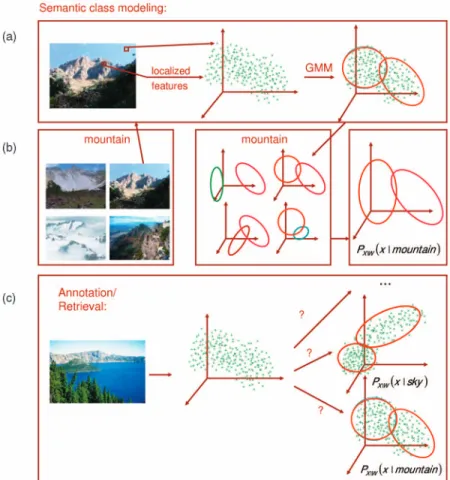
Overall, the proposed implementation of SML leads to optimal(in a minimum probability of error sense)annotation and retrieval, and can be implemented with algorithms that are conceptually simple, computationally efficient, and do not require prior semantic segmentation of training images. Images are simply represented as bags of localized feature vectors, a mixture density estimated for each image, and the mixtures (associated with all images annotated) with a common semantic label pooled into a density estimate for the corresponding semantic class. Semantic annotation and retrieval are then implemented with a minimum probability of error rule, based on these class densities. The overall SML procedure is illustrated in Fig. 1.
Its efficiency and accuracy are demonstrated through an extensive experimental evaluation, involving large-scale databases and a number of state-of-the-art semantic image labeling and retrieval methods. It is shown that SML outperforms existing approaches by a significant margin, not only in terms of annotation and retrieval accuracy, but also in terms of efficiency. This large-scale experimental evaluation also establishes a common framework for the comparison of various methods that had previously only been evaluated under disjoint experimental protocols [5], [6], [12], [13], [21], [23], [29]. This will hopefully simplify the design of future semantic annotation and retrieval systems, by establishing a set of common benchmarks against which new algorithms can be easily tested. Finally, it is shown that SML algorithms are quite robust with respect to the tuning of their main parameters.
The paper is organized as follows: Section 2 defines the semantic labeling and retrieval problems and reviews the supervised OVA and unsupervised formulations. SML is introduced in Section 3 and the estimation of semantic densities is introduced in Section 4. In Section 5, we present the experimental protocols used to evaluate the perfor-mance of SML. Section 6 then reports on the use of these protocols to compare SML to the best known results from the literature. Finally, the robustness of SML to parameter tuning is studied in Section 6 and the overall conclusions of this work are presented in Section 7.
2
S
EMANTICL
ABELING ANDR
ETRIEVALConsider a database T ¼ fI1;. . .;INg of imagesIi and a
semantic vocabulary L ¼ fw1;. . .; wTg of semantic labels
wi. The goal of semantic image annotation is to, given an
image I, extract the set of semantic labels, or caption,1 w
that best describesI. The goal of semantic retrieval is to,
given a semantic label wi, extract the images in the
database that contain the associated visual concept. In
both cases, learning is based on a training set D ¼
fðI1;w1Þ;. . .;ðID;wDÞgof image-caption pairs. The
train-ing set is said to be weakly labeled if 1) the absence of a semantic label from captionwi does not necessarily mean
that the associated concept is not present in Ii, and 2) it
is not known which image regions are associated with 1. A caption is represented by a binary vectorwofTdimensions whose
each label. For example, an image containing “sky” may not be explicitly annotated with that label and, when it is, no indication is available regarding which image pixels actually depict sky. Weak labeling is expected in practical retrieval scenarios, since 1) each image is likely to be annotated with a small caption that only identifies the semantics deemed as most relevant to the labeler, and 2) users are rarely willing to manually annotate image regions. In the remainder of this section, we briefly review the currently prevailing formulations for semantic labeling and retrieval.
2.1 Supervised OVA Labeling
Under the supervised OVA formulation, labeling is
formulated as a collection of T detection problems that
determine the presence/absence of the concepts ofLin the
image I. Consider the ith such problem and the random
variableYi such that
Yi¼
1; ifIcontains conceptwi
0; otherwise:
ð1Þ
Given a collection of q feature vectors X ¼ fx1;. . .;xqg
extracted fromI, the goal is to infer the state ofYiwith the
smallest probability of error, for all i. Using well-known results from statistical decision theory [11], this is solved by declaring the concept as present if
PXjYiðXj1ÞPYið1Þ PXjYiðXj0ÞPYið0Þ; ð2Þ
where Xis the random vector from which visual features are drawn,PXjYiðxjjÞ is its conditional density under class j2 f0;1g, and PYiðjÞ is the prior probability of that class.
Training consists of assembling a training setD1
contain-ing all images labeled with the conceptwi, a training setD0
containing the remaining images, and using some density estimation procedure to estimate PXjYiðxjjÞ from Dj, j2 f0;1g. Note that any images containing concept wi
which are not explicitly annotated with this concept are
incorrectly assigned to D0 and can compromise the
classification accuracy. In this sense, the supervised OVA formulation is not amenable to weak labeling. Furthermore, the setD0 is likely to be quite large when the vocabulary
sizeT is large and the training complexity is dominated by the complexity of learning the conditional density for
Yi¼0.
In any case, (2) produces a sequence of labels ^
wi2 f0;1g; i2 f1;. . .; Tg, and a set of posterior probabilities
PYijXð1jX Þthat can be taken as degrees of confidence on the
annotation of the image with concept wi. Note, however,
that these are posterior probabilities relative to different classification problems and they do not establish an
ordering of importance of the semantic label wi as
descriptors ofI. Nevertheless, the binary decision regard-ing the presence of each concept in the image is a minimum probability of the error decision.
Fig. 1. (a) Modeling of semantic classes. Images are represented as bags of localized features and a Gaussian mixture model (GMM) learned from each mixture. The GMMs learned from all images annotated with a common semantic label (“mountain” in the example above) are pooled into a density estimate for the class. (c) Semantic image retrieval and annotation are implemented with a minimum probability of error rule based on the class densities.
2.2 Unsupervised Labeling
The basic idea underlying the unsupervised learning formulation [3], [4], [12], [13], [15], [21], [31] is to introduce a variableLthat encodes hidden states of the world. Each of these states then defines a joint distribution for semantic labels and image features. The various methods differ in the definition of the states of the hidden variable: Some associate a state to each image in the database [13], [21], while others associate them with image clusters [3], [12], and some model higher-level groupings, e.g., by topic [4]. The overall model is of the form
PX;WðX;wÞ ¼
XS l¼1
PX;WjLðX;wjlÞPLðlÞ; ð3Þ
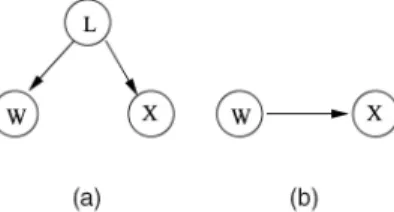
whereSis the number of possible states ofL,Xis the set of feature vectors extracted fromI, andwis the caption of this image. In order to avoid the difficulties of joint inference over continuous and discrete random variables, and as illustrated by the graphical model of Fig. 2a, the visual and text components are usually assumed independent given the state of the hidden variable
PX;WjLðX;wjlÞ ¼PXjLðX jlÞPWjLðwjlÞ: ð4Þ
Since (3) is a mixture model, learning is usually based on the expectation-maximization (EM) [9] algorithm, but the details depend on the particular definition of a hidden variable and the probabilistic model adopted forPX;Wðx;wÞ. The simplest
model in this family [13], [21], which has also achieved the best results in experimental trials, makes each image in the training database a state of the latent variable,
PX;WðX;wÞ ¼
XD l¼1
PXjLðX jlÞPWjLðwjlÞPLðlÞ; ð5Þ
where D is the training set size. This enables individual estimation of PXjLðX jlÞ and PWjLðwjlÞ from each training
image, as is common in the probabilistic retrieval literature [36], [42], [45], therefore eliminating the need to iterate the EM algorithm over the entire database (a procedure of significant computational complexity). It follows that the training complexity is equivalent to that of learning the conditional densities for Yi¼1 in the supervised OVA
formulation. This is significantly smaller than the learning complexity of that formulation (which, as discussed above, is dominated by the much more demanding task of learning the conditionals forYi¼0). The text distributionPWjLðwjlÞ,
l2 f1;. . .; Dgis learned by maximum likelihood, from the annotations of thelthtraining image, usually reducing to a counting operation [13], [21]. Note that, while the quality of the estimates improves when the image is annotated with
all concepts that it includes, it is possible to compensate for missing labels by using standard Bayesian (regularized) estimates [13], [21]. Hence, the impact of weak labeling is not major under this formulation.
At annotation time, (3) is instantiated with the set of feature vectors X extracted from the query I to obtain a function of w that ranks all captions by relevance to the latter. This function can be the joint density of (3) or the posterior density
PWjXðwjX Þ ¼
PX;WðX;wÞ
PXðX Þ
: ð6Þ
Note that, while this can be interpreted as the Bayesian decision rule for a classification problem with the states of
Was classes, such a class structure is not consistent with the generative model of (3) which enforces a causal relationship fromLtoW. Therefore,this formulation imposes a mismatch between the class structure encoded in the generative model (where classes are determined by the state of the hidden variable) and that used for labeling (which assumes that it is the state of W that determines the class). This implies that the annotation decisions are not optimal in a minimum probability of error sense.
Furthermore, when (4) is adopted, this suboptimality is compounded by a very weak dependency between the observationXand captionWvariables, which are assumed independent given L. The significance of the restrictions imposed by this assumption is best understood by example. Assume that the states ofLencode topics, and one of the topics is “bears.” Assume, further, that
1. the topic “bears” is associated with stateL¼b, 2. there are only two types of bear images, “grizzly”
versus “polar” bears,
3. the two types have equal probability under the
“bears” topic,PWjLðgrizzlyjbÞ ¼PWjLðpolarjbÞ ¼1=2,
and
4. the visual features are pixel colors.
Consider next the case where the images to label are those shown in Fig. 3, and let Xi be the set of feature vectors
extracted fromIi; i2 f1;2g. From (4), it follows that
PWjX;LðwjXi; bÞ ¼
PW;XjLðw;XijbÞ
PXjLðXijbÞ
¼PWjLðwjbÞ
and, for both values ofi,
PWjX;LðgrizzlyjXi; bÞ ¼PWjX;LðpolarjXi; bÞ ¼1=2: Fig. 2. Graphical model of the (a) unsupervised and (b) SML models.
Fig. 3. Two images of the “bear” topic. A grizzly bear on the left and a polar bear on the right.
This means that, even though a mostly brown (white) image has been observed, the labeling process still produces the label “polar” (“grizzly”) 50 percent of the time, i.e., with the same frequency as before the observation! Given that the goal of semantic annotation isexactly to learn a mapping from visual features to labels, the assumption of independence given the hidden state is unlikely to lead to powerful labeling systems.
3
S
UPERVISEDM
ULTICLASSL
ABELINGSML addresses the limitations of unsupervised labeling by explicitly making the elements of the semantic vocabulary the classes of a multiclass labeling problem. That is, by introducing 1) a random variableW, which takes values inf1;. . .; Tg, so thatW ¼iif and only ifxis a sample from conceptwi and
2) a set of class-conditional distributions PXjWðxjiÞ; i2 f1;. . .; Tg for the distribution of visual features given the semantic class. The graphical model underlying SML is shown in Fig. 2b. Using, once again, well-known results from statistical decision theory [11], it is not difficult to show that both labeling and retrieval can be implemented with a minimum probability of error if the posterior probabilities
PWjXðijxÞ ¼
PXjWðxjiÞPWðiÞ
PXðxÞ
ð7Þ
are available, where PWðiÞ is the prior probability of the
ithsemantic class. In particular, given a set of feature vectors
X extracted from a (previously unseen) test image I, the minimum probability of an error label for that image is
iðX Þ ¼arg max
i PWjXðijX Þ: ð8Þ
Similarly, given a query conceptwi, a minimum probability
of error semantic retrieval can be achieved by returning the database image of index
jðwiÞ ¼arg max
j PXjWðXjjiÞ; ð9Þ
where Xj is the set of feature vectors extracted from the
jth database image, Ij. When compared to the OVA
formulation, SML relies on a single multiclass problem of
T classes instead of a sequence of T binary detection
problems.
This has several advantages. First, there is no longer a need to estimateT nonclass distributions (Yi ¼0in (1)), an
operation which, as discussed above, is the computational bottleneck of OVA. On the contrary, as will be shown in Section 4, it is possible to estimate all semantic densities
PXjWðxjiÞ with computation equivalent to that required to
estimate one density per image. Hence, SML has a learning complexity equivalent to the simpler of the unsupervised labeling approaches (5). Second, the ith semantic class density is estimated from a training set Di containing all
feature vectors extracted from images labeled with concept wi. While this will be most accurate if all images
that contain the concept includewiin their captions, images
for which this label is missing will simply not be considered. If the number of images correctly annotated is large, this is not likely to make a practical difference. If that number is
small, missing images can always be compensated for by adopting Bayesian (regularized) estimates. In this sense, SML is equivalent to the unsupervised formulation and, unlike supervised OVA, not severely affected by weak labeling.
Third, at annotation time, SML produces an ordering of the semantic classes by posterior probability PWjXðijX Þ.
Unlike OVA, these posteriors are relative to the same classification problem, a problem where the semantic classes compete to explain the query. This ordering is, in fact, equivalent to that adopted by the unsupervised learning formulation (6), but now leads to a Bayesian decision rule that is matched to the class structure of the underlying generative model. It is therefore optimal in a minimum probability of error sense. Finally, by not requiring the modeling of the joint likelihood of words and visual features, SML does not require the independence assumptions usually associated with the unsupervised formulation.
4
E
STIMATION OFS
EMANTICC
LASSD
ISTRIBUTIONSGiven the semantic class densities PXjWðxjiÞ;8i, both
annotation and retrieval are relatively trivial operations. They simply consist of the search for the solution of (8) and (9), respectively, where PWðiÞ can be estimated by the
relative frequencies of the various classes in the database and PXðxÞ ¼PiPXjWðxjiÞPWðiÞ. However, the estimation
of the class densities raises two interesting questions. The first is whether it is possible to learn the densities of semantic concepts in the absence of a semantic segmenta-tion for each image in the database. This is the subject of Section 4.1. The second is computational complexity: If the database is large, the direct estimation ofPXjWðxjiÞfrom the
set of all feature vectors extracted from all images that contain conceptwi is usually infeasible. One solution is to
discard part of the data, but this is suboptimal in the sense that important training cases may be lost. Section 4.2 discusses more effective alternatives.
4.1 Modeling Classes Without Segmentation
Many of the concepts of interest for semantic annotation or retrieval only occupy a fraction of the images that contain them. While objects, e.g., “bear” or “flag,” are prominent examples of such concepts, this property also holds for more generic semantic classes, e.g., “sky” or “grass.” Hence, most images are a combination of various concepts and, ideally, the assembly of a training set for each semantic class should be preceded by 1) careful semantic segmenta-tion, and 2) identification of the image regions containing the associated visual feature vectors. In practice, the manual segmentation of all database images with respect to all concepts of interest is infeasible. On the other hand, automated segmentation methods are usually not able to produce a decomposition of each image into a plausible set of semantic regions. A pressing question is then whether it is possible to estimate the densities of a semantic class without prior semantic segmentation, i.e., from a training set containing a significant percentage of feature vectors from other semantic classes.
We approach this question from a multiple instance learning perspective [2], [10], [20], [27], [28]. Unlike classical learning, which is based on sets of positive and negative examples, multiple instance learning addresses the problem of how to learn models from positive and negative bags of examples. A bag is a collection of examples and is considered positive if at least one of those examples is positive. Otherwise, the bag is negative. The basic intuition is quite simple: While the negative examples present in positive bags tend to be spread all over the feature space, the positive examples are much more likely to be concentrated within a small region of the latter. Hence, the empirical distribution of positive bags is well approximated by a mixture of two components: a uniform component from which negative examples are drawn, and the distribution of positive examples. The key insight is that, because it must integrate to one, the uniform component tends to have small amplitude (in particular, if the feature space is high-dimensional). It follows that, although the density of the common concept may not be dominant in any individual image, the consistent appearance in all images makes it dominant over the entire positive bag.
The principle is illustrated in Fig. 4 for a hypothetical set of images containing four semantic Gaussian concepts, each with probability i2 ½0;1(i.e., occupying i of the image
area). Introducing a hidden variable L for the image
number, the distribution of each image can be written as
PXjLðxjlÞ ¼ X4 i¼1 iG x; li; l i ; ð10Þ
where P4i¼1i¼1, ðli; liÞ are the mean and variance of
the ith Gaussian associated with the lth image, with
Gðx; ; Þ ¼ 1
pffiffiffiffi2e
ðxÞ2 =22
, and the distribution of the bag ofDimages is PXðxÞ ¼ XD l¼1 PXjLðxjlÞPLðlÞ ¼ 1 D XD l¼1 X4 i¼1 iG x; li; l i ;
where we have assumed that all images are equally likely. If one of the four components (e.g., the first, for simplicity) is always the density of concept w, e.g., l1¼
w and l1¼w;8l, and the others are randomly selected
from a pool of Gaussians of uniformly distributed mean and standard deviation, then
PXðxÞ ¼ X4 i¼1 1 D XD l¼1 iG x; li; l i ¼1Gðx; w; wÞ þ X4 i¼2 i D XD l¼1 Gx; li; li
and, from the law of large numbers, asD! 1
PXðxÞ ¼1Gðx; w; wÞ þ ð11Þ
Z
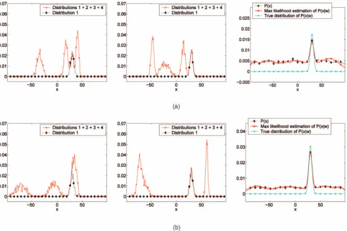
Gðx; ; Þp;ð; Þdd; Fig. 4. Synthetic example of multiple instance learning of semantic class densities. Left and center columns: Probability distributions of individual imagesðPXjLðxjlÞÞ. Each image distribution is simulated by a mixture of the distribution of the concept of interest (dashed line) and three distributions
of other visual concepts present in the image (solid line). All concepts are simulated as Gaussians of different mean and variance. Right column: empirical distribution PXðxÞobtained from a bag ofD¼1;000simulated images, the estimated class conditional distribution (using maximum
likelihood parameter estimates under a mixture of Gaussians model)P^XjWðxjwÞ, and the true underlying distributionPXjWðxjwÞ ¼ Gðx; w; wÞof the
where p;ð; Þ is the joint distribution of the means and
variances of the components other than that associated with
w. Hence, the distribution of the positive bag for conceptw
is a mixture of 1) the concept’s density and 2) the average of many Gaussians of different mean and covariance. The latter converges to a uniform distribution that, in order to integrate to one, must have small amplitude, i.e.,
lim
D!1PXðxÞ ¼1Gðx; w; wÞ þ ð11Þ;
with0.
Fig. 4 presents a simulation of this effect when
2 ½100;100, 2 ½0:1;10, w¼30, w¼3:3, and the
bag contains D¼1;000 images. Fig. 5 presents a
compar-ison between the estimate of the distribution of w,
^
PXjWðxjwÞ, obtained by fitting (in the maximum likelihood
sense) a mixture of five Gaussians (using the EM algorithm [9]) to the entire bag, and the true distribution
PXjWðxjwÞ ¼ Gðx; w; wÞ. The comparison is based on the
Kullback-Leibler (KL) divergence KLðP^XjWkPXjWÞ ¼X x ^ PXjWðxjwÞlog ^ PXjWðxjwÞ PXjWðxjwÞ ;
and shows that, even when 1 is small (e.g.,1¼0:3), the
distribution of conceptwdominates the empirical distribu-tion of the bag, as the numberDof images increases.
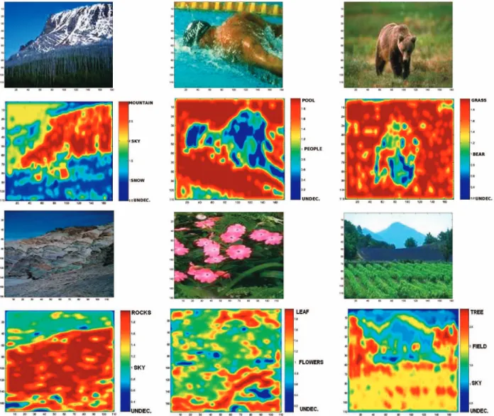
Fig. 6 shows that the same type of behavior is observed in real image databases. In this example, images are represented as a collection of independent feature vectors, as discussed in detail in Section 4.3, and all densities are modeled as Gaussian mixtures. Semantic densities were learned over a set of training images from the Corel database (see Section 6), using the method described in Section 4.2. A set of test images were then semantically segmented by 1) extracting a feature vector from each location in the test image, and 2) classifying this feature vector into one of the semantic classes present in the image (semantic classes were obtained from the caption provided with the image [12]). Fig. 6 depicts the indices of the classes to which each image location was assigned (class indices shown in the color bar on the right of the image) according to
iðXÞ ¼ arg maxiPWjXðijX Þ; ifPWjXðijX Þ>
0; otherwise;
ð11Þ
where X is the set of feature vectors extracted from the image to segment, ¼0:5, PWjXðijX Þ ¼ PXjWðX jiÞPWðiÞ PXðX Þ with PXjWðX jiÞ ¼ Y k PXjWðxkjiÞ; ð12Þ PWðiÞ uniform, PXðXÞ ¼PXjWðX jiÞPWðiÞ þPXjWðXj:iÞPWð:iÞ;
and the density for “no class i” ð:iÞ learned from all training images that did not contain classiin their caption. In order to facilitate visualization, the posterior maps were reproduced by adding a constant, the index of the class of largest posterior, to that posterior. Regions where all posteriors were below threshold were declared “unde-cided.” Finally, the segmentation map was smoothed with a Gaussian filter. Note that, while coarse, the segmentations do 1) split the images into regions of different semantics, and 2) make correct assignments between regions and semantic descriptors. This shows that the learned densities are close to the true semantic class densities.
4.2 Density Estimation
Given the training set Di of images containing conceptwi,
the estimation of the densityPXjWðxjiÞcan proceed in four
different ways: direct estimation, model averaging, naive averaging, andhierarchical estimation.
4.2.1 Direct Estimation
Direct estimation consists of estimating the class density from a training set containing all feature vectors from all images inDi. The main disadvantage of this strategy is that,
for classes with a sizable number of images, the training set is likely to be quite large. This creates a number of practical problems, e.g., the requirement for large amounts of memory, and makes sophisticated density estimation techniques infeasible. One solution is to discard part of the data, but this is suboptimal in the sense that important training cases may be lost. We have not been able to successfully apply this strategy.
4.2.2 Model Averaging
Model averaging exploits the idea of (3) to overcome the computational complexity of direct estimation. It performs the estimation ofPXjWðxjiÞ in two steps. In the first step, a
density estimate is produced for each image, originating a sequencePXjL;Wðxjl; iÞ; l2 f1;. . .Dig, where Lis a hidden
variable that indicates the image number. The class density is then obtained by averaging the densities in this sequence
PXjWðxjiÞ ¼ 1 Di XDi l¼1 PXjL;Wðxjl; iÞ: ð13Þ
Note that this is equivalent to the density estimate obtained under the unsupervised labeling framework if the text
Fig. 5. KL divergence between the estimated, P^XjWðxjwÞ, and actual, PXjWðxjwÞ, class conditional density of conceptwas a function of the
number of training images D, for different values of 1. Error bars
illustrate the standard deviation over a set of 10 experiments for each combination ofD¼ f1; ;1;000gand1¼0:3;0:4.
component of the joint density of (3) is marginalized and the hidden states are images (as in (5)). The main difference is that, while under SML, the averaging is done only over the set of images that belong to the semantic class, under unsupervised labeling, it is done over the entire database. This, once again, reflects the lack of classification optimality of the later.
The direct application of (13) is feasible when the densities PXjL;Wðxjl; iÞ are defined over a (common)
parti-tion of the feature space. For example, if all densities are histograms defined on a partition of the feature spaceSinto
Q cells fSqg; q¼1; ; Q and hqi;l, the number of feature
vectors from classithat land on cellSqfor imagel, then the
average class histogram is simply ^ hqi ¼ 1 Di XDi l¼1 hqi;l:
However, when 1) the underlying partition is not the same for all histograms or 2) more sophisticated models (e.g., mixture or nonparametric density estimates) are adopted, model averaging is not as simple.
4.2.3 Naive Averaging
Consider, for example, the Gauss mixture model
PXjL;Wðxjl; iÞ ¼
X
k
i;lkGx; ki;l;i;lk; ð14Þ
where k
i;l is a probability mass function such that
P
kki;l¼1. Direct application of (13) leads to
PXjWðxjiÞ ¼ 1 Di X k XDi l¼1
i;lkGx; ki;l;i;lk; ð15Þ
i.e., aDi-fold increase in the number of Gaussian
compo-nents per mixture. Since, at annotation time, this probability has to be evaluated for each semantic class, it is clear that straightforward model averaging will lead to an extremely slow annotation process.
4.2.4 Mixture Hierarchies
One efficient alternative to the complexity of model averaging is to adopt a hierarchical density estimation method first proposed in [43] for image indexing. This method is based on a mixture hierarchy where children
Fig. 6. Original images (top row) and posterior assignments (bottom row) for each image neighborhood (Undecided means that no class has a posterior bigger than in (11).).
densities consist of different combinations of subsets of the parents’ components. In the semantic labeling context, image densities are children and semantic class densities are their parents. As shown in [43], it is possible to estimate the parameters of class mixtures directly from those available for the individual image mixtures, using a two-stage procedure. The first two-stage is the naive averaging of (15).
Assuming that each image mixture hasKcomponents, this
leads to a class mixture ofDiKcomponents with parameters
kj; kj;kj
n o
; j¼1;. . .; Di; k¼1;. . .; K: ð16Þ
The second is an extension of EM which clusters the
Gaussian components into anM-componentmixture, where
M is the number of components desired at the class level. Denoting by fm
c; mc;mcg; m¼1;. . .; M the parameters of
the class mixture, this algorithm iterates between the following steps: E-step:Compute hmjk¼ Gð k j; mc ;mcÞe 1 2tracefð m cÞ 1k jg h ik jN m c P l Gðkj; lc; l cÞe 1 2tracefð l cÞ 1 k jg h ik jN l c ; ð17Þ
where N is a user-defined parameter (see [43] for details) set toN ¼1in all our experiments.
M-step:Set ðmcÞnew¼ P jkhmjk DiK ; ð18Þ ðmc Þnew ¼X jk wmjkkj; wherewmjk¼ h m jkkj P jkhmjkkj ; ð19Þ ðmc Þ new ¼X jk wjkmhkjþ ðkjmcÞðjkmcÞTi: ð20Þ
Note that the number of parameters in each image mixture is orders of magnitude smaller than the number of feature vectors in the image itself. Hence, the complexity of estimating the class mixture parameters is negligible when compared to that of estimating the individual mixture parameters for all images in the class. It follows that the overall training complexity is dominated by the latter task, i.e., only marginally superior to that of naive averaging and significantly smaller than that associated with direct estimation of class densities. On the other hand, the complexity of evaluating likelihoods is exactly the same as that of direct estimation and significantly smaller than that of naive averaging.
One final interesting property of the EM steps above is that they enforce a data-driven form of covariance regular-ization. This regularization is visible in (20) where the variances on the left-hand side can never be smaller than those on the right-hand side. We have observed that, due to this property, hierarchical class density estimates are much more reliable than those obtained with direct learning [43].
4.3 Algorithm Description
In this section, we describe the three algorithms used in this work, namely, training, annotation, and retrieval. We also identify the parameters of the training algorithm that affect the performance of the the annotation and retrieval tasks. For the training algorithm, we assume a training set D ¼ fðI1;w1Þ;. . .;ðID;wDÞg of image-caption pairs,
where Ii2 TD with TD¼ fI1;. . .;IDg, and wi L, with L ¼ fw1;. . .; wTg. The steps of the training algorithm are:
1. For each semantic classw2 L,
a. Build a training image setT~D TD, wherew2 wi for allIi2T~D.
b. For each imageI 2T~D,
i. Decompose I into a set of overlapping8
8 regions, extracted with a sliding window that moves by two pixels between con-secutive samples (note that, in all experi-ments reported in this work, images were represented in the YBR color space). ii. Compute a feature vector, at each location of
the three YBR color channels, by the applica-tion of the discrete cosine transform (DCT) (see the Appendix, which can be found on the Computer Society Digital Library at http://computer.org/tpami/archives.htm, for more information). Let the image be represented by B ¼f½xY;xB;xR 1;½x Y;xB;xR 2; . . .;½xY;xB;xR Mg; where ½xY;xB;xR m is the concatenation of
the DCT vectors extracted from each of the YBR color channels at image location
m2 f1;. . .; Mg. Note that the 192-dimen-sional YBR-DCT vectors are concatenated by interleaving the values of the YBR feature components. This facilitates the application of dimensionality reduction techniques due to the well-known energy compaction properties of the DCT. To simplify notation, we hereafter replace
½xY;xB;xRwithx.
iii. Assuming that the feature vectors extracted
from the regions of image I are sampled
independently, find the mixture of eight Gaussians that maximizes their likelihood using the EM algorithm [9] (in all experi-ments, the Gaussian components had diag-onal covariance matrices). This produces the following class conditional distribution for each image: PXjWðxjI Þ ¼ X8 k¼1 kIG x; kI;k I ; ð21Þ
where kI; kI;kI are the maximum like-lihood parameters for imageI and mixture componentk.
c. Fit a Gaussian mixture of 64 components by applying the hierarchical EM algorithm of (17)-(20) to the image-level mixtures of (21). This leads to a conditional distribution for classwof
PXjWðxjwÞ ¼ X64 k¼1 k wG x; kw;kw :
We refer to this representation as GMM-DCT. The parameters that may affect labeling and retrieval perfor-mance are 1) number of hierarchy levels on step (1-c), 2) number of DCT feature dimensions, and c) number of mixture components for the class hierarchy in step (1-c). The number of hierarchical levels in (1-c) was increased from two to three in some experiments by adding an intermediate level that splits the image mixtures into groups of 250 and learns a mixture for each of these groups. In Section 6, we provide a complete study of the performance of our method as a function of each one of those parameters.
The annotation algorithm processes test imagesIt62 TD,
executing the following steps:
1. Step (1-b-i) of the training algorithm. 2. Step (1-b-ii) of the training algorithm. 3. For each classwi2 L, compute
logPWjXðwijBÞ ¼logPXjWðBjwiÞ þlogPWðwiÞ logPXðBÞ;
where B is the set of DCT features extracted from imageIt,
logPXjWðBjwiÞ ¼
X
x2B
logPXjWðxjwiÞ;
PWðwiÞ is computed from the training set as the
proportion of images containing annotationwi, and
PXðBÞis a constant in the computation above across
differentwi2 L.
4. Annotate the test image with the five classes wi of
largest posterior probability,logPWjXðwijBÞ.
Finally, the retrieval algorithm takes as inputs 1) a semantic classwi, and 2) a database of test imagesTT, such
thatTTTTD¼ ;. It consists of the following steps:
1. For each image It2 TT, perform steps 1)-4) of the
annotation algorithm.
2. Rank the images labeled with the query word by
decreasingPWjXðwijBÞ.
We have found, experimentally, that the restriction to the images for which the query is a top label increases the robustness of the ranking (as compared by the simple ranking by label posterior,PXjWðBjwiÞ).
5
E
XPERIMENTALP
ROTOCOLAs should be clear from the discussion of the previous sections, a number of proposals for semantic image annotation and retrieval have appeared in the literature. In general, it is quite difficult to compare the relative performances of the resulting algorithms due to the lack of
evaluation on a common experimental protocol. Since the implementation and evaluation of a labeling/retrieval system can be quite time-consuming, it is virtually impossible to compare results with all existing methods. Significant progress has, however, been accomplished in the recent past by the adoption of a “de facto” evaluation standard, that we refer to as Corel5K, by a number of research groups [12], [13], [21].
There are, nevertheless, two significant limitations associated with the Corel5K protocol. First, because it is based on a relatively small database, many of the semantic labels in Corel5K have a very small number of examples. This makes it difficult to guarantee that the resulting annotation systems have good generalization. Second, because the size of the caption vocabulary is also relatively small, Corel5K does not test the scalability of annotation/ retrieval algorithms. Some of these limitations are corrected by the Corel30K protocol, which is an extension of Corel5K based on a substantially larger database. None of the two protocols is, however, easy to apply to massive databases, since both require the manual annotation of each training image. The protocol proposed by Li and Wang [23] (which we refer to as PSU) is a suitable alternative for testing large-scale labeling and retrieval systems.
Because each of the three protocols has been used to characterize a nonoverlapping set of semantic labeling/ retrieval techniques, we evaluated the performance of SML on all three. In addition to enabling a fair comparison of SML with all previous methods, this establishes a data point common to the three protocols that enables a unified view of the relative performances of many previously tested systems. This, we hope, will be beneficial to the community. We describe the three protocols in the remainder of this section and then present the results of our experiments in the following.
5.1 The Corel5k and Corel30k Protocols
The evaluation of a semantic annotation/labeling and retrieval system requires three components: an image database with manually produced annotations, a strategy to train and test the system, and a set of measures of retrieval and annotation performance. The Corel5K bench-mark is based on the Corel image database [12], [13], [21]: 5,000 images from 50 Corel Stock Photo CDs were divided into a training set of 4,000 images, a validation set of 500 images, and a test set of 500 images. An initial set of model parameters is learned on the training set. Parameters that require cross-validation are then optimized on the validation set, after which, this set is merged with the training set to build a new training set of images. Noncross-validated parameters are then tuned with this training set. Each image has a caption of one to five semantic labels, and there are 371 labels in the data set.
Image annotation performance is evaluated by comparing the captions automatically generated for the test set, with the human-produced ground-truth. Similarly to [13], [21], we define the automatic annotation as the five semantic classes of largest posterior probability, and compute the recall and precision of every word in the test set. For a given semantic descriptor, assuming that there are wH human annotated
wC are correct, recall and precision are given byrecall¼wwHC
andprecision¼ wC
wauto, respectively. As suggested in previous
works [13], [21], the values of recall and precision are averaged over the set of words that appear in the test set. Finally, we also consider the number of words with nonzero recall (i.e., words with wC>0), which provides an indication of how many
words the system has effectively learned.
The performance of semantic retrieval is also evaluated by measuring precision and recall. Given a query term and the topnimage matches retrieved from the database, recall is the percentage of all relevant images contained in the retrieved set, and precision is the percentage ofnwhich are relevant (where relevant means that the ground-truth annotation of the image contains the query term). Once again, we adopted the experimental protocol of [13], evaluating retrieval performance by the mean average precision (MAP). This is defined as the average precision, over all queries, at the ranks, where recall changes (i.e., where relevant items occur).
The Corel30K protocol is similar to Corel5K but sub-stantially larger, containing 31,695 images and 5,587 words. Of the 31,695 images, 90 percent were used for training (28,525 images) and 10 percent for testing (3,170 images). Only the words (950 in total) that were used as annotations for at least 10 images were trained. Corel30K is much richer than Corel5K in terms of number of examples per label and database size, therefore posing a much stronger challenge to nonscalable systems.
5.2 The PSU Protocol [23]
For very large image sets, it may not even be practical to label each training image with ground-truth annotations. An alternative approach, proposed by Li and Wang [23], is to assign images to loosely defined categories, where each category is represented by a set of words that characterize the category as a whole, but may not accurately characterize each individual image. For example, a collection of images of tigers running in the wild may be annotated with the words “tiger,” “sky,” “grass,” even though some of the images may not actually depict sky or grass. We refer to this type of annotation as noisy supervised annotation. While it reduces the time required to produce ground-truth annota-tions, it introduces noise in the training set, where each image in some category may contain only a subset of the category annotations.
Li and Wang [23] relied on noisy supervised annotation to label very large databases by implementing a 2-step annotation procedure, which we refer to as supervised category-based labeling (SCBL). The image to label is first processed with an image category classifier that identifies the five image categories to which the image is most likely to belong. The annotations from those categories are then pooled into a list of candidate annotations with frequency counts for reoccurring annotations. The candidate annota-tions are then ordered based on the hypothesis test that a candidate annotation has occurred randomly in the list of candidate annotations.
More specifically, the probability that the candidate
word appears at least j times in k randomly selected
categories is Pðj; kÞ ¼X k i¼j IðimÞ m i nm ki n k ;
whereIð:Þis the indicator function,nis the total number of image categories, andmis the number of image categories containing the word. For n; mk, the probability can be approximated by Pðj; kÞ X k i¼j k i pið1pÞki;
where p¼m=n is the frequency with which the word
appears in the annotation categories. A small Pðj; kÞ
indicates a low probability that the candidate word occurred randomly (i.e., the word has high significance as an annotation). Hence, candidate words withPðj; kÞbelow a threshold value are selected as the annotations.
Li and Wang [23] also proposed an experimental protocol, based on noisy supervised annotation for the evaluation of highly scalable semantic labeling and retrieval systems. This protocol, which we refer to as PSU, is also based on the Corel image set, containing 60,000 images with 442 annotations. The image set was split into 600 image categories consisting of 100 images each, which were then annotated with a general description that reflected the image category as a whole. For performance evaluation, 40 percent of the PSU images were reserved for training (23,878 images), and the remainder (35,817 images) were used for testing. Note that Li and Wang [23] only used 4,630 of the 35,817 possible test images, whereas all the test images were used in the experiments reported here. Annotation and retrieval perfor-mance were evaluated with the same measures used in Corel5K and Corel30K.
6
E
XPERIMENTALR
ESULTSIn this section, we compare the performance of SML with the previous approaches discussed above. We start with a comparison against the less scalable unsupervised labeling methods, using the Corel5K setup. We then compare SML to SCBL on the larger PSU benchmark. Finally, we perform a study of the scalability and robustness of SML. The experiments reported here were conducted on a cluster of 3,000 state-of-the-art Linux machines. Some of these experiments involved extensive replication of a baseline experiment with various configurations of the free para-meters of each retrieval system. In the most extreme cases, computing time was as high as 1 hour for Corel5K and 34 hours for PSU, although these times are not definitive since the experiments ran concurrently with, and were preempted by, other jobs on the cluster.
6.1 Comparison of SML and Unsupervised Labeling
Table 1 presents the results obtained for SML and various previously proposed methods (results from [13], [21]) on Corel5K. Specifically, we considered the co-occurrence model of [29], the translation model of [12], the contin-uous-space relevance model of [13], [21], and the multiple-Bernoulli relevance model (MBRM) of [13]. Overall, SML achieves the best performance, exhibiting a gain of 16 percent in recall for an equivalent level of precision when compared
to the previous best results (MBRM). Furthermore, the number of words with positive recall increases by 15 percent. Fig. 7 presents some examples of the annotations produced. Note that, when the system annotates an image with a descriptor not contained in the human-made caption, this annotation is frequently plausible.
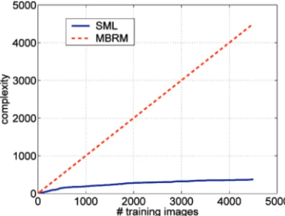
We next analyze the complexity of the annotation
process. Assuming that there are D training images and
each produces Rvisual feature vectors, the complexity of
CRM and MBRM is OðDRÞ. On the other hand, SML has
complexity of OðT RÞ, where T is the number of semantic classes (or image annotations), and is usually much smaller
than D. For example, Fig. 8 presents the per-image
annotation time required by each of the methods on the Corel data set, as a function of D. Note the much smaller rate of increase, with database size, of the SML curve.
The performance of semantic retrieval was evaluated by measuring precision and recall as explained in Section 5.1. Table 2 shows that, for ranked retrieval on Corel, SML produces results superior to those of MBRM. In particular, it achieves a gain of 40 percent mean average precision on the set of words that have positive recall. Fig. 9 illustrates the retrieval results obtained with one word queries for challenging visual concepts. Note the diversity of visual appearance of the returned images, indicating that SML has good generalization ability.
6.2 Comparison of SML and SCBL
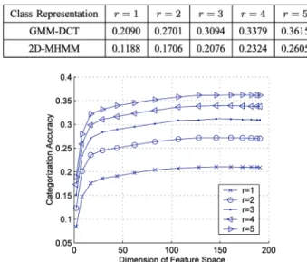
To evaluate the performance of SML on large-scale retrieval and annotation tasks, we compared its performance to that of SCBL under the PSU protocol. For this, we started by comparing the image categorization performance between the GMM-DCT class representation described in Section 4.3 and the representation of [23]. In [23], an image category is represented by a two-dimensional multiresolution hidden Markov model (2D-MHMM) defined on a feature space of localized color and wavelet texture features at multiple scales. An image was considered to be correctly categorized if any of the toprcategories is the true category. Table 3 shows the accuracy of image categorization using the two class representations. GMM-DCT outperformed the 2D-MHMM of [23] in all cases, with an improvement of about 0.10 (from 0.26 to 0.36). Fig. 10 shows the categorization accuracy of GMM-DCT versus the dimension of the DCT feature space. It can be seen that the categorization accuracy increases with the dimension of the feature space, but remains fairly stable over a significant range of dimensions.
TABLE 1
Performance Comparison of Automatic Annotation on Corel5K
Fig. 7. Comparison of SML annotations with those of a human subject.
Fig. 8. Comparison of the time complexity for the annotation of a test image on the Corel data set.
We next compared the annotation performance of the two steps of SCBL, using the GMM-DCT representation (we denote this combination by SCBL-GMM-DCT) and [23]. Following [23], the performance was measured using “mean coverage,” which is the percentage of ground-truth annotations that match the computer annotations. Table 4 shows the mean coverage of SCBL-GMM-DCT and of [23] using a threshold of 0.0649 on Pðj; kÞ, as in [23], and without using a threshold. Annotations using GMM-DCT outperform those of [23] by about 0.13 (from 0.22 to 0.34 using a threshold, and 0.47 to 0.61 for no threshold). Fig. 11 shows the mean coverage versus the dimension of the DCT feature space. Again, performance increases with feature space dimension, but remains fairly stable over a large range of dimensions.
Finally, we compared SCBL and SML when both methods used the GMM-DCT representation. SCBL annota-tion was performed by thresholding the hypothesis test
(SCBL-GMM-DCT threshold), or by selecting a fixed number annotations (SCBL-GMM-DCT fixed). SML classi-fiers were learned using both 2-level and 3-level hierarchies. Fig. 12 presents the precision-recall (PR) curves produced by
TABLE 2
Retrieval Results on Corel5K
Fig. 9. Semantic retrieval on Corel. Each row shows the top five matches to a semantic query. From top to bottom:“blooms,” “mountain,” “pool,” “smoke,”and“woman.”
TABLE 3
Accuracy of Image Categorization on the PSU Database
Fig. 10. Accuracy of image categorization on PSU using GMM-DCT versus the dimension of the DCT feature space.
the two methods. Note that SML trained with the 3-level hierarchy outperforms the 2-level hierarchy. This is evi-dence that the hierarchical EM algorithm provides some
regularization of the density estimates, which improves the performance. The SML curve has the best overall precision at 0.236, and its precision is clearly superior to that of SCBL at most levels of recall. There are, however, some levels where SCBL-GMM-DCT leads to a better precision. This is due to the coupling of words within the same image category and to the noise in the ground-truth annotations of PSU.
Note that if the correct category is in the top five classified categories, then the list of candidate words will contain all of the ground-truth words for that image. Eventually, as the image is annotated with more words from the candidate list, these ground-truth words will be included, regardless of whether the ground truth actually applies to the image (i.e., when the ground truth is noisy). As a result, recall and precision are artificially inflated as the number of annotations increases. On the other hand, for SML, each word class is learned separately from the other words. Hence, images will not be annotated with the noisy word if the concept is not present, and the precision and recall can suffer. Finally, for SCBL-threshold, the PR curve has an unusual shape. This is an artifact that arises from thresholding a hypothesis test that has discrete levels.
In summary, the experimental results show that the GMM-DCT representation substantially outperforms the 2D-MHMM of [23] in both image categorization and annotation using SCBL. When comparing SML and SCBL based on the GMM-DCT representation, SML achieves the best overall precision, but for some recall levels, SCBL can achieve a better precision due to the coupling of annotation words and noise in the annotation ground truth.
6.3 Robustness and Scalability of SML
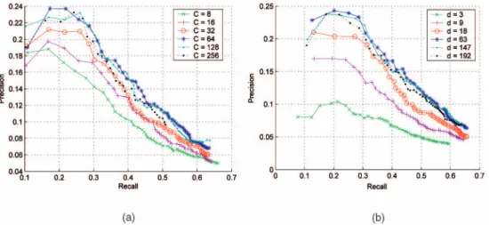
We have already seen that, under the SCBL model, both the categorization and annotation performance of the GMM-DCT representation are quite stable with respect to the feature space dimension. We now report on experiments performed to evaluate the robustness of SML-GMM-DCT method to its tunable parameters. Fig. 13a shows the PR curves obtained for annotation on Corel5K, as a function of the number of mixture components used to model class conditional densities. Note that the PR curve remains fairly
TABLE 4
Mean Coverage for Annotation on the PSU Database
Fig. 11. Mean coverage of annotation of PSU using SCBL-GMM-DCT versus the dimension of the DCT feature space.
Fig. 12. Precision-Recall for SCBL and SML using GMM-DCT on the PSU database.
Fig. 13. Precision-recall curves for annotation on Corel5K using SML-GMM-DCT while varying: (a) the number of mixture componentsðCÞand (b) the dimension of the DCT feature spaceðdÞfor 64 mixture components.
stable above 64 components. Fig. 13b shows the PR curve for annotation with 64 components while varying the feature space dimension. In this case, stability is achieved above 63 dimensions.
To test scalability, the SML annotation experiment was repeated on the larger Corel30K. Fig. 14 shows the performance obtained with 64 and 128 mixture compo-nents, learned with either the 2-level or 3-level hierarchy. The first observation that can be made from the figure is that a 3-level hierarchy outperforms the standard 2-level hierarchy for both 64 and 128 components. This indicates that the density estimates achieved with the 3-level structure are superior to those of the standard hierarchical organization. The differences are nevertheless not stagger-ing, suggesting some robustness of SML with respect to this parameter. A second interesting observation is that annota-tion performance on the larger database is qualitatively similar to that obtained on the smaller Corel5K database (e.g., compare the shape of the PR curves with those of Fig. 13a), albeit with overall lower precision and recall levels. This is due to the difficulty of learning specialized annotations, and to the presence of different annotations with the same semantic meaning, which are both more frequent on Corel30K. It appears likely that the absolute values of PR could be improved by complementing SML
with a language model which accounts for the multiple labels that can usually be assigned to the same semantic concept (e.g., “car” versus “automobile” versus “vehicle,” etc.). These types of operations are routinely done in textual information retrieval (e.g., through the application ofquery expansiontechniques [1]) and could be easily combined with SML. We believe that this is an interesting topic for further research.
Overall, these experiments indicate that 1) SML is fairly stable with respect to its parameter settings, and 2) results on Corel5K are a good indication of the relative perfor-mance of different techniques on larger databases (albeit the absolute values of PR are likely to be overestimated).
6.4 Ranked Retrieval Results
Fig. 15 presents results of ranked retrieval on Corel5K for different numbers of mixture components and DCT dimensions. Fig. 15a depicts the MAP for all 260 words, while the one in the center shows the same curves for words with nonzero recall. In both cases, the MAP increases with the number of mixture components, stabilizing above 128 components. Fig. 15b shows the number of words with nonzero recall, which decreases with the number of mixture components, once again stabilizing above 128 components.
7
C
ONCLUSIONSIn this work, we have presented a unifying view of state-of-the-art techniques for semantic-based image annotation and retrieval. This view was used to identify limitations of the different methods and motivated the introduction of SML. When compared with previous approaches, SML has the advantage of combining classification and retrieval optimality with 1) scalability in database and vocabulary sizes, 2) ability to produce a natural ordering for semantic labels at annotation time, and 3) implementation with algorithms that are conceptually simple and do not require prior semantic image segmentation. We have also pre-sented the results of an extensive experimental evaluation, under various previously proposed experimental proto-cols, which demonstrated superior performance with respect to a sizable number of state-of-the-art methods, for both semantic labeling and retrieval. This experimental
Fig. 14. Precision-recall curves for annotation on Corel30K using SML-GMM-DCT.
Fig. 15. Ranked retrieval on Corel5K using SML-GMM-DCT with different mixture componentsðCÞ: (a) MAP for all the words, (b) MAP for words with nonzero recall, and (c) number of words with nonzero recall.
evaluation has also shown that the performance of SML is quite robust to variability in parameters such as the dimension of the feature space or the number of mixture components.
A
CKNOWLEDGMENTSThe authors would like to thank Kobus Barnard for providing the Corel5K data set used in [12], David Forsyth for providing the Corel30K data set, James Wang for the PSU data set used in [23], and Google Inc. for providing the computer resources for many of the experiments. This research was partially supported by the US National Science Foundation CAREER award IIS-0448609 and a grant from Google Inc. Gustavo Carneiro also wishes to acknowledge funding received from NSERC (Canada) to support this research. Finally, they would like to thank the reviewers for insightful comments that helped to improve the paper. Gustavo Carneiro developed this work while he was with the Statistical Computing Laboratory at the University of California, San Diego.
R
EFERENCES[1] R. Attar and A. Fraenkel, “Local Feedback in Full-Text Retrieval Systems,”J. ACM,vol. 24, no. 3, pp. 397-417, July 1977.
[2] P. Auer, “On Learning from Multi-Instance Examples: Empirical Evaluation of a Theoretical Approach,” Proc. 14th Int’l Conf. Machine Learning,pp. 21-29, 1997.
[3] K. Barnard and D. Forsyth, “Learning the Semantics of Words and Pictures,”Proc. Int’l Conf. Computer Vision,vol. 2, pp. 408-415, 2001.
[4] D. Blei and M. Jordan, “Modeling Annotated Data,”Proc. ACM SIGIR Conf. Research and Development in Information Retrieval,2003.
[5] G. Carneiro and N. Vasconcelos, “Formulating Semantic Image Annotation as a Supervised Learning Problem,”Proc. IEEE Conf. Computer Vision and Pattern Recognition (CVPR),2005.
[6] G. Carneiro and N. Vasconcelos, “A Database Centric View of Semantic Image Annotation and Retrieval,” Proc. ACM SIGIR Conf. Research and Development in Information Retrieval,2005.
[7] J. De Bonet and P. Viola, “Structure Driven Image Database Retrieval,” Proc. Conf. Advances in Neural Information Processing Systems,vol. 10, 1997.
[8] P. Carbonetto, N. de Freitas, and K. Barnard, “A Statistical Model for General Contextual Object Recognition,”Proc. European Conf. Computer Vision,2004.
[9] A. Dempster, N. Laird, and D. Rubin, “Maximum-Likelihood from Incomplete Data via the EM Algorithm,”J. Royal Statistical Soc.,vol. B-39, 1977.
[10] T. Dietterich, R. Lathrop, and T. Lozano-Perez, “Solving the Multiple Instance Problem with Axis-Parallel Rectangles,” Artifi-cial Intelligence,vol. 89, nos. 1-2, pp. 31-71, 1997.
[11] R. Duda, P. Hart, and D. Stork,Pattern Classification.John Wiley and Sons, 2001.
[12] P. Duygulu, K. Barnard, and D.F.N. Freitas, “Object Recognition as Machine Translation: Learning a Lexicon for a Fixed Image Vocabulary,”Proc. European Conf. Computer Vision,2002.
[13] S. Feng, R. Manmatha, and V. Lavrenko, “Multiple Bernoulli Relevance Models for Image and Video Annotation,”Proc. IEEE CS Conf. Computer Vision and Pattern Recognition,2004.
[14] D. Forsyth and M. Fleck, “Body Plans,” Proc. IEEE CS Conf. Computer Vision and Pattern Recognition,pp. 678-683, 1997.
[15] P. Carbonetto, H. Kueck, and N. Freitas, “A Constrained Semi-Supervised Learning Approach to Data Association,” Proc. European Conf. Computer Vision,2004.
[16] N. Haering, Z. Myles, and N. Lobo, “Locating Dedicuous Trees,”
Proc. Workshop in Content-Based Access to Image and Video Libraries,
pp. 18-25, 1997.
[17] J. Hafner, H. Sawhney, W. Equitz, M. Flickner, and W. Niblack, “Efficient Color Histogram Indexing for Quadratic Form Distance Functions,”IEEE Trans. Pattern. Analysis and Machine Intelligence,
vol. 17, no. 7, pp. 729-736, July 1995.
[18] J. Huang, S. Kumar, M. Mitra, W. Zhu, and R. Zabih, “Spatial Color Indexing and Applications,”Int’l J. Computer Vision,vol. 35, no. 3, pp. 245-268, Dec. 1999.
[19] A. Jain and A. Vailaya, “Image Retrieval Using Color and Shape,”
Pattern Recognition J.,vol. 29, pp. 1233-1244, Aug. 1996.
[20] A. Kalai and A. Blum, “A Note on Learning from Multiple Instance Examples,”Artificial Intelligence,vol. 30, no. 1, pp. 23-30, 1998.
[21] V. Lavrenko, R. Manmatha, and J. Jeon, “A Model for Learning the Semantics of Pictures,”Proc. Conf. Advances in Neural Information Processing Systems,2003.
[22] Y. Li and L. Shapiro, “Consistent Line Clusters for Building Recognition in CBIR,”Proc. Int’l Conf. Pattern Recognition,vol. 3, pp. 952-956, 2002.
[23] J. Li and J. Wang, “Automatic Linguistic Indexing of Pictures by a Statistical Modeling Approach,”IEEE Trans. Pattern Analysis and Machine Intelligence,vol. 25, no. 9, pp. 1075-1088, Sept. 2003.
[24] F. Liu and R. Picard, “Periodicity, Directionality, and Random-ness: Wold Features for Image Modeling and Retrieval,”IEEE Trans. Pattern Analysis and Machine Intelligence, vol. 18, no. 3, pp. 722-733, July 1996.
[25] B. Manjunath and W. Ma, “Texture Features for Browsing and Retrieval of Image Data,”IEEE Trans. Pattern Analysis and Machine Intelligence,vol. 18, no. 8, pp. 837-842, Aug. 1996.
[26] R. Manmatha and S. Ravela, “A Syntactic Characterization of Appearance and Its Application to Image Retrieval,”Proc. SPIE Conf. Human Vision and Electronic Imaging II,vol. 3016, 1997.
[27] O. Maron and T. Lozano-Perez, “A Framework for Multiple-Instance Learning,” Proc. Conf. Advances in Neural Information Processing Systems,vol. 10, 1997.
[28] O. Maron and A. Ratan, “Multiple-Instance Learning for Natural Scene Classification,” Proc. 15th Int’l Conf. Machine Learning,
pp. 341-349, 1998.
[29] Y. Mori, H. Takahashi, and R. Oka, “Image-to-Word Transforma-tion Based on Dividing and Vector Quantizing Images with Words,”Proc. First Int’l Workshop Multimedia Intelligent Storage and Retrieval Management,1999