Market Concentration, Macroeconomic Uncertainty and Monetary Policy.

Full text

(1)Market Concentration, Macroeconomic Uncertainty and Monetary Policy. Juan de Dios Tena Francesco Giovannoni. Discussion Paper No. 05/576. August 2005. Department of Economics University of Bristol 8 Woodland Road Bristol BS8 1TN.

(2) Market Concentration, Macroeconomic Uncertainty and Monetary Policy∗ Juan de Dios Tena†. Francesco Giovannoni‡. August 2005. Abstract This paper studies the effect of market structure and macroeconomic uncertainty on the transmission of monetary policy. We motivate our analysis with a simple model which predicts that: 1) investment and production in more concentrated sectors are more affected by demand changes and 2) high uncertainty makes investment and production more sensitive to demand changes. The empirical analysis estimates the effect of monetary shocks on sectoral output for different sectors in the US using different structural vector autoregressive VAR approaches. The results are largely consistent with the proposed theory. Keywords: Market concentration, macroeconomic uncertainty, monetary policy transmission, vector autoregressive models. JEL Codes: E22, E32, E52, D43.. ∗. We would like to thank Jon Temple,Andy Tremayne, Daniel Seidmann, Alex Cuckierman, Zvi Hercowitz,. Daniel Tsiddon, Yona Rubinstein, partecipants the 2005 World Congress of the Econometric Society and seminar partecipants at Tel Aviv University, Bank of Israel, Universita’ di Sassari and the University of Newcastle for helpful comments and suggestions. We also thank CMPO for Þnancial support. The usual qualiÞer applies. †. Universidad de Concepcion, Departamento de Economia, Victoria 471 - OÞcina 242 - Concepcion, Chile and. Universita’ degli Studi di Sassari, Dipartamento di Economia e Impresa, via Torre Tonda, 34 - 07100 Sassari, Italy. E-mail: juande@udec.cl ‡. Department of Economics and CMPO, University of Bristol, 8 Woodland Rd., Bristol, BS8 1TN, UK. E-mail:. francesco.giovannoni@bristol.ac.uk.

(3) 1. Introduction In this paper, we stress the relevance of product market structure for the monetary transmission mechanism with particular emphasis on investment decisions. We develop the intuition through a simple model where Þrms choose their investment and pricing strategies as a function of the degree of market concentration in their industry. The model shows how different levels of market concentration explain different investment and production reactions to changes in demand. Further, we also show that uncertainty about future demand can have a signiÞcant impact on investment because it affects market structure. Our theory differs from the previous literature on the monetary transmission mechanism, for which we can identify two separate strands. The Þrst of these, emphasizes the presence of “frictions” in credit markets. The idea is that asymmetric information in credit markets leads to differences between the costs of internal and external Þnance that depend on the Þnancial position of the borrowers. As a consequence, the effect of monetary shocks is highly correlated with the business cycle: in risky periods, Þnancial restrictions are more likely and will tend to impact Þrms for which credit market imperfections are more signiÞcant. The second strand emphasizes the importance of uncertainty when investment is irreversible.1 One feature that is common to both these approaches is that they often ignore how Þrms interact in the market and how expected proÞt is affected by this interaction because they either focus on the behavior of individual Þrms or on a group of Þrms in a perfectly competitive product market. Our focus on market structure, on the other hand, suggests an alternative to the credit restriction theories while underlying the implication of our analysis for investment under uncertainty. More speciÞcally, in the model we consider an industry where potential investors have access to idiosyncratic investment opportunities in capacity. These investments can either be made in the present or at some future period, when there will be some uncertainty about demand. The number of potential investors that has access to such opportunities is a crucial parameter in our model as it captures the degree of concentration in the industry: the smaller this number, the more concentrated the industry will be. Although investment opportunities are individualspeciÞc, the model is entirely symmetric as all potential investors face the same opportunity cost of investment, the same capacity level if they make the investment, the same (zero) marginal cost of production, the same discount factor between periods and the same market demand for the (identical) Þnal product. In each period, investment decisions are made simultaneously by those who have not invested in the previous period. In a given period, those who do invest, proceed to simultaneously select prices. Thus, investment decisions in the present are made by comparing expected proÞts if the investment is postponed until the future with the expected proÞts if the investment is made in the present. 1. In the next section we review the literature more thoroughly.. 2.

(4) Our Þrst result is that greater market concentration makes investment decisions more sensitive to changes in present and future demand. The intuition is particularly simple: greater concentration implies higher proÞts for each investor in each period. This means that, for example, an expected increase in future demand, will increase the opportunity cost of investing today and not in the future more than it would have if smaller proÞts were at stake. While simple, this result establishes an unambiguous link between market concentration on the one hand, and monetary policy and its impact on demand, on the other. Our other results concern the effects of uncertainty on investment. As we will discuss in detail below, a negative correlation between future uncertainty and present investment is well established in the literature, both from a theoretical and empirical perspective, but our model suggests that these effects may be mediated by the degree of market concentration. In particular, we show that when uncertainty is so high that a negative shock to demand will signiÞcantly alter market structure, then the effect on today’s investment is stronger than when uncertainty is low and a change in market structure following a demand shock is not likely. In other words, today’s investment decisions are more sensitive to changes in the uncertainty about future demand, the greater this uncertainty is to begin with. The intuition is that whenever shocks to future demand are so large as to have an impact on market structure, then there is an increase in the value of the option of postponing investment decisions until the uncertainty is realized. We proceed to take the predictions of the model to the data, by considering the effects of monetary shocks on industrial production for different manufacturing sectors in the United States. In order to do this, we follow the traditional macroeconomic literature in assuming that monetary policy drives demand shocks. We consider monthly data from 1972 to 2003 for a group of 21 United States manufacturing sectors classiÞed according to the North American Standard Industrial ClassiÞcation System (NAICS). The focus on United States sectors will help us in identifying the impact that market concentration in each sector has on the monetary transmission mechanism since this is the least open economy in the OECD.2 We use a VAR approach to estimate the effect of unexpected interest rate changes on sectoral output. Although VAR speciÞcations are not based on economic theory, they have become a common tool for the sectoral analysis of monetary transmission.3 One advantage of this methodology lies in the fact that all the fundamental variables are endogenously determined in the system. Thus, a structural model is identiÞed and the effect of unanticipated monetary policy changes can be estimated. This overcomes some of the problems found in the parameter interpretation of reduced form equations where demand shifts fail to be exogenous as they can be anticipated 2. According to the OECD Main Economic Indicators, in 2002, imports plus exports in the United States were. 18.3% as a share of GDP. The only country that compares is Japan with 19%, while other major OECD countries such as Germany (51.5%), France (42.9%), Italy (41.5%) and the United Kingdom (39.9%) are much more open. 3. See for example Gertler and Gilchrist, [13] and [14], and Dedola and Lippi [9].. 3.

(5) by economic agents. The literature (and indeed the data) suggests that output volatility in the United States has signiÞcantly decreased from the second half of the eighties, following the changes introduced by the Monetary Control Act of 1980 and the Garn-St. Germain Act of 1982. Consistent with this view, we estimate industrial reactions to interest rate shocks in two VAR models: one for the period from the beginning of 1972 to the end of 1982 and one for the period up to 2003. In order to assure the robusteness of our results, we also consider a Threshold VAR (TVAR) approach. A novel feature of introduced by this speciÞcation is that it allows uncertainty to change all the possible relations amongst fundamentals in the model. A second feature is that we utilize the methodology developed by Koop et al. [23] to estimate impulse-response functions in nonlinear models and adjusted by Atanasova [2] to threshold vector autoregressive (TVAR) systems. With this methodology once a shock occurs, the model is allowed to switch from one uncertainty regime to the other according to the underlying process followed by macroeconomic uncertainty. Our results are largely compatible with the intuitions developed in the theoretical model. We Þnd that the intensity of the reactions in a given sector depend positively on its degree of market concentration while several proxies related to the credit and interest rate channel are not as signiÞcant. We also Þnd that macroeconomic uncertainty increases sensitivity to interest rate shocks but the evidence is weaker. This paper is organized as follows. The next section relates our work to the previous literature. A simple model is presented in Section 3. The purpose of the model is not to provide a complete description of the monetary transmission mechanism, but to provide some insights into how market concentration may interact with changes in demand and uncertainty about future prospects. Section 4 presents the data. Section 5 discusses the econometric approach we use for the estimation of sectoral reactions to interest rate shocks while section 6 presents the results and considers the impact of market concentration. Conclusions are drawn in Section 7. We relegate more technical matters to the appendix.. 2. Related Literature In this section we discuss in detail the connections between the two main approaches to the monetary transmission mechanism and our analysis. As mentioned above, the Þrst approach emphasizes the role of imperfections in credit markets. Some prominent examples can be found in Kiyotaki and Moore [21], Kiyotaki [22] or Bernanke and Gertler [4]. In their models, asymmetric information in the credit market leads to a difference between the cost of internal and external Þnance that depends on the Þnancial position of the borrowers. If this happens, sequentially uncorrelated shocks can generate correlated economic ßuctuations. For example, a positive shock. 4.

(6) may positively affect investment by affecting entrepreneurial net worth as income increases. The expansion persists because the rise in capital stock makes investment in future periods higher than it would otherwise be. For this reason, the term “Þnancial accelerator” (Bernanke et al. [3]) has been used to refer to the magniÞcation of the initial shocks by Þnancial market imperfections. These theoretical models imply non-linear dynamics and asymmetric responses to monetary policy shocks. In particular, a given change in monetary policy is likely to have a stronger effect in volatile periods as it can alleviate Þnancial constraints. The models also imply crosssectional differences in the transmission of monetary policy for different Þrms or industrial sectors depending on their access to the credit market. The second approach focuses on the role of irreversible investment decisions under uncertainty as developed by Dixit and Pindyck [11]. Their important contribution was the recognition that option pricing theory provides insights into investment decisions that go beyond the traditional net present value rule whenever investors face uncertainty about relevant future states of the world and when decisions are irreversible. According to this theory, for an investment to be made, its net present value must be sufficiently large to cover the value to investors of delaying their investment and keeping the investment option alive. Following this approach, a number of papers have studied the link between uncertainty, irreversibility and investment decisions both from the perspective of individual Þrms and at the industry level; see for example Dixit [10] and Abel and Eberly [1] for the case of individual Þrm decisions and idiosyncratic uncertainty and Leahy [24] and Caballero and Pindyck [6] for the case of investment decisions at the industry level. Importantly, Caballero and Pindyck [6] argue that when studying irreversible investment in an industry context, only aggregate uncertainty can alter investment decisions by Þrms. The reason is that, assuming free entry of new Þrms, only aggregate shocks have an asymmetric effect on the expected investment returns. This asymmetry arises because although negative shocks reduce market price, the entry of new Þrms after a positive shock prevents any increase in proÞts. This framework offers, at least, two relevant intuitions for our analysis. First, because of the aforementioned truncation in the expected outcome of investment, uncertainty reduces the optimal amount of investment in capital.4 Second, to study the role of imperfect competition in the model, they consider an isoelastic demand curve. In their model, an increase in the elasticity of demand implies that the potentially positive effects of the failing units on the price is reduced. This lowers expected revenue ßow and also raises the trigger point at which Þrms are willing to invest. We also consider the impact of uncertainty on investment decisions at the industry level 4. However, note that this result is not unanimous in the literature. For example, Abel and Eberly [1] pinpoint. that due to irreversibility constraints, after an adverse shock a Þrm would like to sell capital but cannot. This effect tends to increase the Þrm’s capital stock and makes the link between investment and uncertainty ambiguous.. 5.

(7) in a simple partial-equilibrium two-period model. Our novel contribution is that instead of assuming an isoelastic demand function, we have that the pricing strategies adopted by the Þrms, the effective level of competition and its associated proÞts, are obtained from Þrst principles as a function of the degree of market concentration. Irreversibility comes from the fact that productivity units are only allowed to invest in one of the two periods. A main result in our model is that the effect of positive and negative shocks is asymmetric but the type of asymmetry is of a different nature to the one studied by Caballero and Pindyck [6]. In our model expected proÞts have a lower bound at zero due to the fact that the pricing strategy adopted by the Þrms is an endogenous decision that depends on the capacity of the industry. Effectively, price cannot be lower than marginal cost of production regardless of the intensity of the negative shock. However, if there are frictions in the entry of new Þrms expected proÞts can always increase after a positive shock. Given that the opportunity to invest presents itself only once, uncertainty increase the value of waiting and investing in the future. The literature has already empirically investigated the possible impact of a number of different factors in order to explain the heterogenous impact of monetary shocks on real activity. For example, Gertler and Gilchrist ([13] and [14]) argue that different access to credit markets can explain the differences in investment behavior between large and small Þrms. The idea is that large Þrms are more likely to have access to commercial paper markets and other source of credit, and this makes them more likely to respond to a non-anticipated decline in cash ßow by increasing short term borrowing. Gertler and Gilchrist Þnd that the inventories of large Þrms grow following a tightening of monetary policy. This indicates that larger Þrms can (at least temporarily) maintain their levels of production in the face of an increase in real interest rates and proÞts. In contrast, small Þrms, which normally have more limited access to short term credit markets, respond to unanticipated monetary contractions principally by reducing inventories and cutting production. Dale and Haldane [8], on the other hand, Þnd stronger investment reactions to monetary shocks for the corporate sector over the personal sector, using UK data. The Gertler and Gilchrist evidence has found further support in a recent article by Dedola and Lippi [9] who document and analyze sectoral output reactions for 5 OECD countries. They also Þnd that additional Þnancial (and nonÞnancial) factors are important elements in explaining monetary transmission. For example, they Þnd that sectors which produce durable goods tend to have smaller reactions. We follow Dale and Haldane [8] and Dedola and Lippi [9] in the use of sectoral data, but in contrast to them, we estimate the effect of monetary shocks in high and low uncertainty periods and focus on market concentration as the crucial explanatory variable for the heterogeneity of reactions across industries. Our result that higher market concentration in a sector increases reactions in that sector to monetary shocks contrasts with theories which predict that demand shocks have a stronger and longer lasting impact in sectors dominated by small Þrms as our data 6.

(8) shows that more concentrated sectors tend to have larger Þrms. Just like our theory, the credit constraint theories predict that demand shocks have a bigger impact in high uncertainty periods. Clearly the two stories are different: in our model, higher uncertainty works through its effect on market structure, while in the credit constraints literature, higher uncertainty worsens informational asymmetries. Our results provide some evidence that the link between market concentration and responses to monetary shocks is enhanced by higher macroeconomic uncertainty, while variables related to informational asymmetries seem to have little explanatory power. This would suggests that market concentration plays a bigger role in the monetary transmission mechanism that variables associated with credit restrictions. Finally, our results also contrast with some of the predictions of the Abel and Eberly [1] setup. If we take the predictions of their model to the issue of monetary transmission, we would expect that uncertainty increases the user cost of capital which, in turn, reduces the responsiveness of both the decision to invest and the amount of investment to monetary shocks. As mentioned above, our data suggest that for our sectors, the opposite occurs.. 3. The Model We consider the behavior of a group of producers in a single industrial sector. We assume there is a set {1, ..., m} of such potential producers (which we index by i), and each of them has to decide. whether or not to undertake an investment in capacity. We assume that a producer has one and only one single, indivisible and idiosyncratic investment opportunity: this is to keep matters simple by assuring that producers cannot sell any part of their projects to others. Also, for simplicity, we assume that there are two periods in which to take up the investment opportunity and that the investment only generates income for the period in which it is undertaken.. Every investment opportunity has sunk cost c and gives the investor the capacity to produce a maximum of 1 unit of a Þnal good q. If the investment is not made in a given period, then potential producer i gets zero proÞts for that period. Expected proÞts in period 2 are discounted by a factor δ ∈ (0, 1) in period 1. We let N t represent the set of potential producers who do undertake investment in period t ∈ {1, 2} and let nt represent its cardinality. Given our. assumptions, it must be that n1 + n2 ≤ m.. The Þnal good produced is perfectly homogeneous and, for all investors, marginal cost of. production is zero. (Inverse) market demand for the Þnal good in period t is a linear function pt = at − Qt P whenever at −Qt ≥ 0 and zero otherwise, where at > 1 and Qt = i∈N qit . This simple formulation. for demand leads to manageable comparative statics. We will also assume that c < at −1 because this guarantees that a producer that expects to be a monopolist in a given period, will always have an incentive to invest. 7.

(9) Given these assumptions, our simple timeline is as follows: 1. In period 1, potential producers simultaneously decide whether to undertake their idiosyncratic investment. This determines N 1 . 2. Producers i ∈ N 1 simultaneously Þx a price p1i for their Þnal good. Given the price vector, quantities qi1 are determined. We assume that each investor faces demand qi1 = a1 − p1i. whenever p1i is the lowest price, while the surplus maximizing rationing rule is used whenever p1i is not the lowest price.5 3. In period 2, those potential producers who did not invest in period 1, simultaneously decide whether to undertake their idiosyncratic investment now. This determines N 2 . 4. Given N 2 , competition between all those who have invested ensues as described in 2. Given these assumptions, we can analyze the price-setting subgame for a given value of nt determined in 1 and 3. Since this is a simply a Bertrand-Edgeworth game with linear demand, symmetric capacities and constant marginal costs, results follow directly from Levitan and Shubik [26] and a fully detailed version is omitted. In the appendix, we provide a sketch, along the lines of Vives [38], to show how mixed strategies are calculated. ¢ ¡ ¡ ¢ Lemma 1 Equilibrium prices pti i∈N t and the corresponding level of expected proÞts Eπti i∈N t are given by:. 1. If nt ≥ at + 1 pti = 0 for all i ∈ N t. Eπti = 0 for all i ∈ N t 2. If 1 ≤ nt ≤ at − 1 pti = at − nt for all i ∈ N t. Eπti = at − nt for all i ∈ N t 5. In our context, the surplus-maximizing rationing rule requires that contingent demand for investor i, given. that L investors charge a lower price than p1i and S investors charge exactly p1i be equal to ¢ 1¡ 1 a − p1i − L S. 8.

(10) 3. If at − 1 < nt < at + 1, then all producers play a mixed strategy with distribution function £ ¤ F t and support pt , pt , where at − nt + 1 2 µ t ¶2 a − nt + 1 pt = 2 ! t1 Ã t − pt n −1 ¡ ¢ p F t pt = pt (pt + nt − at ) pt =. where expected proÞts from this strategy are equal to Eπti =. ³. at −nt +1 2. ´2. for all i ∈ N t .. Lemma 1 states that in any given period, pricing strategies depend crucially on the number of investments in capacity made in that period. In particular, the number of investments determine three regimes. In the Þrst regime, the number of investments is relatively large. This makes competition so strong that prices will be set at marginal cost (zero). In the second regime, relatively few investments are made and this reduced competition leads each investor to be able to sell his full capacity at a high price. Finally, in the third regime we have an intermediate number of investments. In this case, investors are indifferent between selling all their capacity at a price pt and acting as a monopolist on the residual demand left by the other investors. Thus, £ ¤ they will choose a mixed strategy, represented by F t where they charge a price pt ∈ pt , pt but won’t sell their full capacity.. Once optimal pricing strategies are determined, we can analyze the optimal investment decisions themselves. Given the symmetry of the proÞt function for all producers, we can simply ¡ ¢ indicate with Eπt nt the expected proÞts for a producer given that there are other nt − 1 producers in the market. Following Seade [30], we now treat the variables nt as continuous variables. but restrict attention to integer realizations when necessary. Lemma 2 Suppose c > 0. In any subgame-perfect equilibrium of the game, the sets of potential ¢ ¡ 1 2 that decide to enter in periods 1 and 2 respectively, are always such that if producers Neq , Neq ¡ 1 2¢ n e ,n e are values for which ¡ 1¢ ¡ ¡ 2¢ ¢ e − c = δ Eπ2 n e −c =0 Eπ1 n. ¡ ¢ ¡ 1 2¢ ¢ ¡ then n1eq , n2eq = n e ,n e1 + n e whenever n e2 ≤ m. If n e1 + n e2 > m then n1eq , n2eq are such that ¡ ¢ ¡ ¡ ¢ ¢ Eπ1 n1eq − c = δ Eπ2 n2eq − c > 0. Proof. Consider stage 3 and let m−n1 be the number of potential entrants left. It is immediate to see that given that Eπ2 is a strictly decreasing function of n whenever positive, in any equilibrium ¡ 2¢ n2 is such that if n e2 is the value for which Eπ2 n e2 whenever n e2 + n1 ≤ m and e = c then n2 = n 9.

(11) n2 = m − n1 otherwise. Consider now stage 1 where again Eπ2 is a strictly decreasing function of ¡ 1¢ n whenever positive. If n e1 is the value for which Eπ1 n e2 ≤ m, then clearly e − c = 0 and n e1 + n. these will be the equilibrium cardinalities for the two sets of entrants. Suppose, however, that ¡ 1¢ ¡ ¡ ¢ ¢ e −c = 0 while δ Eπ2 m − n e1 − c > n e1 +e n2 > m. Then, if n1 = n e1 , we would have that Eπ1 n. 0 so that an entrant in period 1 would have an incentive to deviate and enter in period 2 instead. ¡ ¢ ¡ ¡ ¢ ¢ It is immediate to see that only equilibria where Eπ 1 n1eq − c = δ Eπ2 n2eq − c are possible. ¤. Lemma 2 provides a simple no-arbitrage condition: in any equilibrium, investment decisions much be such that there is no difference between expected proÞts in each period. One important implication that these expected proÞts will be positive whenever m is sufficiently small. This is a realistic assumption in a variety of circumstances. For example, barriers to access to capital markets, industry regulation, investment irreversibility or lack of infrastructure can all contribute to a de facto limit on the number of participants in a speciÞc market. For our purposes, however, the assumption that m is sufficiently small as to effectively constrain entry, allows a distinction between investment decisions in the short-run where market concentration matters most, and investment decisions in the long-run. Further, we can explicitly derive these effects. To keep matters simple, we will look at those cases where the parameters are such as to guarantee that nteq ≤ at − 1 for t = 1, 2 or to guarantee that at + 1 > nteq > at − 1 for t = 1, 2. This will be true whenever both a1 and a2 are close to each other and/or δ is sufficiently close to one but our. qualitative results are robust to cases in which the market structure differs across periods. Our Þrst result states that whenever markets are more concentrated, short run investment decisions are more sensitive to changes in present demand. Proposition 3 For the case in which n e1 + n e2 > m we have that whenever nteq ≤ at − 1 for t = 1, 2 then. ∂n1eq 1 = 1 ∂a 1+δ. and. ∂n1eq 1 =− 2 ∂a 1+δ. Further, the case in which, at + 1 > nteq > at − 1, for t = 1, 2 will obtain for a value of c. sufficiently close to zero. So, evaluating the equivalent derivatives for c = 0, we get ∂n1eq 1 √ = 1 ∂a 1+ δ. and. ∂n1eq 1 √ =− 2 ∂a 1+ δ. Proof. Follows from simple differentiation of the equilibrium values of investment ¤ From Lemma 2 we know that higher levels of concentration (low m) imply smaller values of n1eq .. Thus, equilibrium proÞts are higher in equilibrium. Given that the stakes are high, a change. in current demand has more dramatic effects on investment decisions than in a less concentrated sector. Note that since entry is restricted, this result also implies that the effect of an increase of present demand on future investment will be opposite to the effect described above. 10.

(12) We can further extend our results by introducing uncertainty in future demand. In our context, where we have just two periods, we capture the simplest possible demand uncertainty by assuming that demand in period 2 will be a2 + σ with probability 1/2 and a2 − σ with complementary probability. Note that our results below rely crucially on our assumption of. restricted entry. If m is unconstrained, uncertainty about the future does not affect investment decisions today. The reason is that in this case investment would always be equal to sunk costs regardless of the level of proÞts expected. To further simplify our analysis, we assume that nteq ≤ at − 1 and evaluate our comparative statics at c = 0.6 Note that n2eq ≤ a2 − 1 implies. n2eq ≤ a2 − 1 + σ so that a positive shock to demand in the second period does not alter market. structure. On the other hand, it does not imply that n2eq ≤ a2 − 1− σ; indeed for sufficiently large values of σ a negative shock can change the pricing regime and the potential for proÞts in the. future by affecting the investment decisions. The following proposition shows that investment is negatively related to uncertainty in future periods. This negative correlation between uncertainty and investment can also be found in McDonald and Siegel [27] or Dixit and Pindyck [11], amongst others. The difference is that here demand uncertainty impacts investment indirectly through its effect on pricing strategies. To get an intuition for the result, consider two extreme cases: in one case uncertainty σ is arbitrarily small and in the other it is arbitrarily large. In the Þrst case, perspective investors who have to decide whether to invest in period 1 or 2, know that in period 2, they face a gamble where the certainty equivalent is approximately equal to the proÞts for the average demand a2 . In the second case, however, the certainty equivalent is much larger than the proÞts for the average demand a2 because proÞts not bounded above but are bounded below by zero. In other words, if uncertainty is above a certain threshold, the value of the option to delay investment increases. Proposition 4 Given the parameter restrictions described above,     0 if σ ≤ σ∗    ¡ ¡ ¢¢  ∂n1eq  δ n2eq − a2 − σ − 1 ¡ ¢ = if σ∗ < σ < σ∗∗ 2 − (a2 − σ + 3) − 4  ∂σ δ n  eq     δ   − <0 if σ ≥ σ∗∗ 2+δ. where σ∗ = a2 − n2eq − 1 and σ∗∗ = a2 − n2eq + 1.. Proof. It is easy to see that if σ ≤ σ∗ , then n1eq is given by the following equality: £ ¡ ¡ ¡ ¢¢ ¡ ¢¢¤ a1 − n1eq = δ 12 a2 + σ − m − n1eq + 12 a2 − σ − m − n1eq 6. The case in which at + 1 > nteq > at − 1 is considerably more complex from a computational perspective. The. same message emerges, although in this case both positive and negative shocks can have an impact. This means that when we apply our results to the data, we should not expect asymmetries between negative and positive shocks.. 11.

(13) which gives us an expression for n1eq which is independent of σ. If σ∗ < σ < σ∗∗ , then market structure in the second period depends on the realization of demand uncertainty. Thus, the corresponding expression is  a1 − n1eq. ¡ ¡ ¢¢ = δ  12 a2 + σ − m − n1eq +. 1 2. Ã. !2  ¡ ¢ a2 − σ − m − n1eq + 1  2. By implicit differentiation, we get the result above. Finally, if σ ≥ σ ∗∗ , market structure changes. further for the case in which second-period demand turns out to be low. We now have the corresponding expression a1 − n1eq = δ. ¢¢ £1 ¡ 2 ¡ 1 + 2 a + σ − m − neq. 1 2. ×0. By solving for n1eq and differentiating we get the desired result ¤. ¤. It is easy to see by considering the appropriate constraints, that ¡ ¢¢ ¡ δ n2eq − a2 − σ − 1 δ ¢ < ¡ 2 − 2+δ δ neq − (a2 − σ + 3) − 4. which means that the (negative) effect gets stronger as uncertainty increases until the maximum effect is reached at the threshold σ ∗∗ . Intuitively, at this point demand is so low that all Þrms in the second period market set prices equal to zero and they cannot go fall further even if market demand further decreases. From the analysis above we can easily recover the effect of a change in Þrst-period demand in the three uncertainty regimes. The following proposition shows that there isn’t just a direct effect of uncertainty on investment, but, crucially, also an indirect effect through changes in current demand. Intuitively, what is happening is that, as discussed above, high levels of uncertainty about future demand reduce investment today. This increases the monopolistic power of those who do invest in the Þrst period. As we’ve seen above, in markets where monopolistic power is higher, the expected proÞts of Þrms are more sensitive to changes in the economic environment. Proposition 5 Given the parameter restrictions described   1     1+δ    ∂n1eq 4 ¡ ¢ >0 =  ∂a1 4 − δ n2eq − (a2 − σ + 3)      2   2+δ. above, if. σ ≤ σ∗. if. σ∗ < σ < σ∗∗. if. σ ≥ σ∗∗. Proof. The same procedure as in the proof of the previous proposition applies ¤ 12.

(14) As before, it is easy to see that our restrictions imply that 2 1 4 ¡ ¢> > 2 2 2+δ 1 + δ 4 − δ neq − (a − σ + 3) In the rest of paper we will take two of our main results to the data. SpeciÞcally, we will study the following predictions of the model: 1. Changes in demand have more impact in more concentrated markets (proposition 3) 2. Changes in demand have more impact whenever uncertainty about future prospects is higher (proposition 5).. 4. Data and Measures of Macroeconomic Uncertainty This section presents the data in the analysis and describes its main features. We Þrst consider time series data at the aggregate and at the sectoral level. At the aggregate level, we use monthly data from January 1972 to December 2003 obtained from the Federal Reserve Bank of Saint Louis. The variables of interest are the Þrst differences (∆Rt ) of the 30-year Conventional Mortgage rate to account for economic agents’ expectations about future inßation; the Þrst differences (∆ot ) in the Industrial Production Index as a measure of output growth; the Consumer Price Index for all Urban Consumers as measure of inßation (πt ); and Þrst differences (∆it ) in the Bank Prime Loan Rate as a measure of changes in the short run interest rate. All variables, except for Rt and it are expressed in natural logarithms before differences are taken.7 At the sectoral level, we consider monthly data for the same period for 21 manufacturing sectors classiÞed according to the North American Industry ClassiÞcation System (NAICS). In this case we utilize Þrst differences of the natural logarithm of the variable “Industrial Production”.8 7. Dale and Haldane [8] also use the long run interest rate as a proxy for expectations about future inßation.. There are many candidates for the choice of a measure of it and qualitatively our results do not change when other measures are used. The aggregated data is freely available on the web site http://research.stlouisfed.org. 8. This data is seasonally adjusted and freely available from http://www.federalreserve.gov. The following sectors. are considered in the analysis: Food(NAICS311); Beverage and Tobacco Product (NAICS312); Textile Mills (NAICS313) ; Textile Product Mills (NAICS314); Apparel (NAICS315); Leather and Allied Product (NAICS316); Wood Product (NAICS321); Paper (NAICS322); Printing and Related Support Activities (NAICS323); Petroleum and Coal Products (NAICS324); Chemical (NAICS325); Plastics and Rubber Product (NAICS326); Non Mineral Metallic Product (NAICS327); Primary Metal (NAICS331); Fabricated metal product (NAICS332); Machinery (NAICS333); Computer and Electronic Product (NAICS334); Electrical Equipment, Appliance, and Component (NAICS335); Transportation Equipment (NAICS336); Furniture and Related Products (NAICS337); Miscellaneous (NAICS339).. 13.

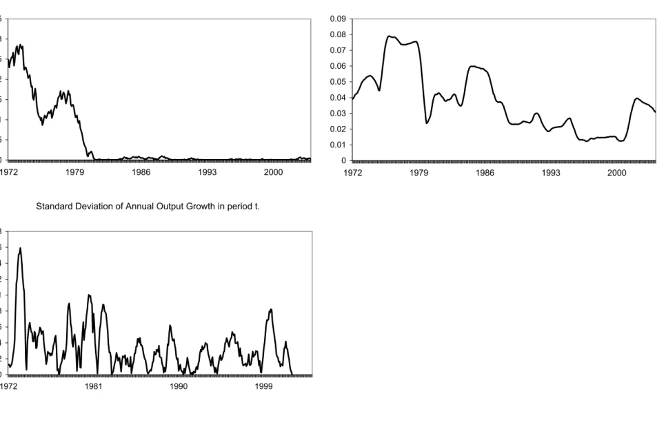
(15) We also use a cross section of measures of market concentration for the same sectors. The main variables of interest are the HerÞndal index and the share of value added accounted for the 4, 8, 20 and 50 largest companies in each sector in 1997.9 We will also introduce cross sectional controls but these are discussed in more detail in section 6. Finally, we need to include a measure of macroeconomic uncertainty. Since there is no universal consensus on the appropriate measure to use, we consider different alternatives. We Þrst consider the rolling standard deviation of the natural logarithm of annual growth ∆12 ot of the industrial production index, with a window of four years. This means that the standard deviation for month t is the estimated standard deviation from months t − 47 to t.. Thus, our Þrst observation for ∆12 ot refers to growth in the year up to February 1968 while the Þrst value of our measure is January 1972, compatibly with the rest of our data. See Blanchard and Simon [5] for a similar approach. An alternative measure is the variance of aggregate output estimated using a GARCH model.10 The GARCH model is speciÞed as:. ot = α00 zt + εt σ2t. = c. + φ1 ε2t−1. (4.1) + φ2 σ2t−1. + α01 zt. (4.2). where zt is the (kx1) vector of our aggregate macroeconomic variables; α0 and α1 are (kx1) vectors of parameters; c, φ1 and φ2 are scalar parameters; σ2t is the conditional variance; and εt is a white noise error. Variables whose parameters are not signiÞcant at the 0.05 level are dropped from the regressions with a stepwise procedure, but changes to the speciÞcations have only limited effects on the estimation of the conditional variance. As a Þnal alternative, we consider the average of the annual growth for the whole period January 1972-December 2003 and for each observation t we use the standard deviation between ∆12 ot and the average. All measures show that on average the variability of output has been decreasing signiÞcantly in the last 20 years of our sample. This is a consistent result in the literature (again, see Blanchard and Simon [5]). Figure 1 shows the three measures. [INSERT FIGURE 1 HERE]. 5. Empirical Analysis In our empirical analysis, we seek to evaluate the asymmetric effects of monetary shocks on industrial output as a function of the underlying macroeconomic uncertainty. We later use these 9 10. This data is available from http://www.census.gov See Price [29] for a similar approach.. 14.

(16) results to study the role of market concentration for different manufacturing sectors in the United States. In order to perform the Þrst task, we consider two different approaches. We specify two different linear VAR models. The Þrst model considers the sample for the period 1972:1-1982:12 while the second considers the sample for remaining period 1983:1-2003:12. We distinguish these two periods as periods of high uncertainty (the former) and low uncertainty (the latter). We chose to spilt the sample at the beginning of 1983 because this follows closely the changes introduced by the Monetary Control Act of 1980 and the Garn-St. Germain Act of 1982 that contributed to drastically reduce output volatility.11 As Þgure 1 shows, our measures of macroeconomic uncertainty all seem to support the decision to set a cut-off in the early 1980s. A Þrst potential problem with the VAR methodology developed here, is that we split the sample according to the criterion described above. Clearly, however, some periods before 1983 could be easily classiÞed as low uncertainty periods and other periods after 1983 could be classiÞed as high uncertainty periods. A second, more fundamental, issue is estimating reaction functions in two separate VAR models amounts to assuming that once a shock occurs, the systems remains in the same (low or high uncertainty) state forever. Our TVAR approach offers a solution to these two problems. In the Þrst instance, they can determine endogenously whether a period is one of high or low uncertainty. Also, we follow the procedure in Koop et al. [23] to obtain impulse response function. Under this procedure, once a shock occurs, the model keeps track of the underlying uncertainty process and this allows the model to switch from one state to the other according to this underlying process. This section presents a brief discussion of the speciÞcation and estimation of our VAR models and its use for the estimation of impulse response functions. In the next section, we document our results and discuss how our measure of market concentration correlates with them. Our TVAR analysis is described in the appendix.. 5.1. VAR Models Vector autoregressive (VAR) models, as advocated by Sims [32], have become a familiar tool in the analysis of monetary transmission mechanisms. We discuss identiÞcation of structural VAR models following along the lines of Christiano et al. [7]. We estimate two reduced form models:   p X ¡ ¢0 Yt1 = Φ10 + Φ1j Yt−j  + a1t and Ea1t a1t = Σ1 for t ∈ T − (5.1) . 11. Yt2 = Φ20 +. See Stock and Watson [34].. j=1. p X j=1. . ¡ ¢0 Φ2j Yt−j  + a2t and Ea2t a2t = Σ2 for t ∈ T +. 15.

(17) where p is the number of lags, Yt is a (5x1) vector of endogenous variables, including ∆Rt , ∆ot , πt , ∆it and changes in “Industrial Production” in those sectors for which we wish to estimate the reaction. In addition, Φ1j and Φ2j are polynomial matrices, a1t and a2t are (5x1) vectors of zero mean, serially uncorrelated disturbances while T − represents all observations up to 1982:12 and T + all observations in 1983:1-2003:12. These models do not allow for the computation of the dynamic response function of Ytk (for k = 1, 2) to the fundamental shocks in the economy. This is because the elements of akt are, in general, contemporaneously correlated and we cannot presume that they solely correspond to a single economic shock. To deal with this issue, we consider two structural models deÞned by A10 Yt1. 1. = Λ +. A20 Yt2 = Λ2 +. p X j=1 p X j=1. A1j Yt−j + ε1t for t ∈ T −. (5.2). A2j Yt−j + ε2t for t ∈ T +. ¡ ¢0 ¡ ¢0 where Eεkt εkt = Ak0 Σk Ak0 = I, is a 5th order matrix. The paramer matrices and errors in ¡ ¢−1 k k ¡ k ¢−1 k ¡ ¢−1 k 5.1 and 5.2 are linked by Φki = Ak0 Ai , Φ0 = A0 Λ and akt = Ak0 εt with εkt being a. (5x1) vector of orthogonal and standardized structural disturbances.. Once consistent estimators of the Φki ’s in (5.1) are obtained, one can estimate Σk from the Þtted residuals. All the information about the matrix Ak0 is contained in the relationship Σk = ¡ k ¢−1 ³¡ k ¢−1 ´0 A0 A0 . However, Ak0 has 25 parameters while the symmetric matrix, Σk , has at most 15 distinct elements.. In order to identify the structural model one usually imposes a set of linear restrictions across the elements of the individual rows of Ak0 . The concomitant order condition, (i), speciÞes that it is necessary to specify at least 10 restrictions, to get a sufficient condition for identiÞcation. Together with this condition, it is necessary, (ii), that the diagonal elements of Ak0 be positive. However, these conditions are still not sufficient for identiÞcation. It is also necessary to ensure, (iii), that a neighbourhood of Ak0 cannot contain other matrices that fulÞl the aforementioned conditions. This is ensured by imposing the additional restriction that the matrix derivative with respect to Ak0 of the equations deÞning Σ is of full rank. By doing this, local identiÞcation is established. For global identiÞcation it is necessary to impose that there not be other matrices that fulÞl the three restrictions (i)-(iii) in a neighbourhood of Ak0. However, if the identiÞcation problem only involves systems of linear equations, local identiÞcation obtains if, and only if, global identiÞcation obtains. When the model is identiÞed, assuming Ytk to be covariance-stationary, one can use model (5.2) to compute the responses of variables in Ytk to fundamental shocks in different periods. Thus, computing impulse response functions in the linear case is straightforward as dynamic response functions of Ytk to fundamental shocks can be obtained analytically from the moving average representation of model (5.2). 16.

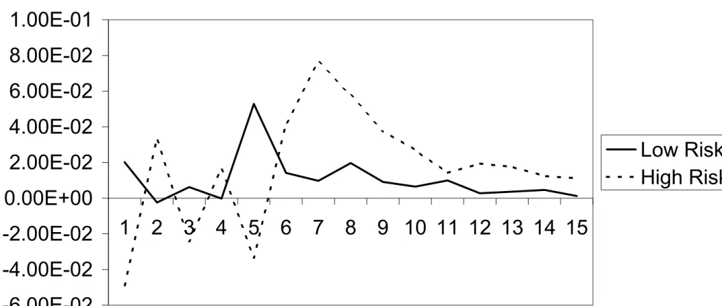
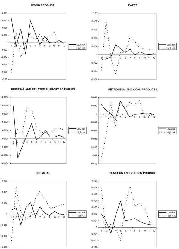
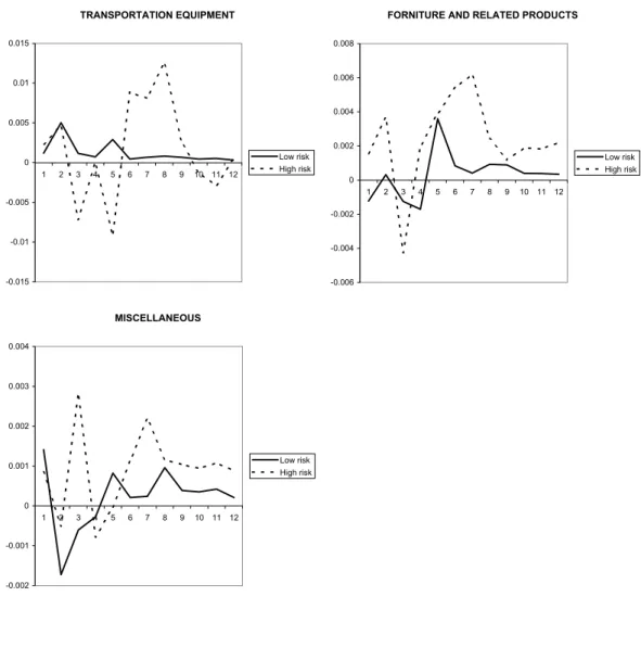
(18) 6. Analysis of the Empirical Results We begin by discussing the impulse response functions obtained through our VAR analysis. These represent the sectoral reactions of industrial output to short run interest shocks for periods of low and high uncertainty respectively. In order to select the number of lags, we applied the Schwartz criterion to the VAR models at the aggregate level and compared the cases in which p = 2 to 6. The criterion weakly supports the choice of p = 4 and this is the case we present here.12 We should point out, however, that we also ran our analysis for the p = 2 case. The differences with the main case are discussed below.13 In Þgures 2-6 we show Þrst the sum of the response functions for all sectors and then the response function for each sector.. [INSERT FIGURES 2-6 HERE] Figure 2 shows that an expansionary monetary shock generates an increase in output in both the high and low uncertainty regimes but the effect in the former case is signiÞcantly larger. At the sectoral level, in Þgures 3-6, we Þnd cross sectional implications. For example, the effect in the Fabricated Metal Products sector is signiÞcantly smaller than the effect in the Transportation Equipment or in the Beverages and Tobacco Products sectors. There are also signiÞcant differences with regard to the timing of the reactions and the high and low uncertainty regimes, although in almost all sectors the high uncertainty regimes seems to be more reactive to the shocks, a result which is compatible with our theoretical model. Given these asymmetries due to macroeconomic uncertainty, we proceed by focusing Þrst on analyzing the heterogeneity of reactions in the low uncertainty period and then we move on to study the effect of high macroeconomic uncertainty. In the high uncertainty period, two main results stand out. First, and consistently with standard macroeconomic theory, the Þgures show that after an adjustment period, reactions tend to be positive until about twelve months when they fade. The perverse responses found in the Þrst Þve or six months for many sectors are not new in the VAR literature: Christiano [7] and Sims [33] document cases of responses that are not consistent with economic theory in the short run. The most likely explanation for this is that the monetary authority sets policy by using private information that is not shared by the rest of the economy and cannot be captured in a VAR model. To further quantify the output effect of monetary shocks across sectors, we consider the maximum industrial output elasticity (MAXE) recorded after the shocks as a measure of intensity. In order to study the role of market share, we also we computed MS4 for each sector, the share 12. SpeciÞcally, for the 1972:1-1982:12 sample, the Schwartz criterion gives -24.5 to all cases. For the 1983:1-. 2003:12 sample, the criterion gives -29.6 to the p = 4 case and -29.5 to all other cases. 13. All the analysis discussed below but not explicitly reported in the paper is available upon request.. 17.

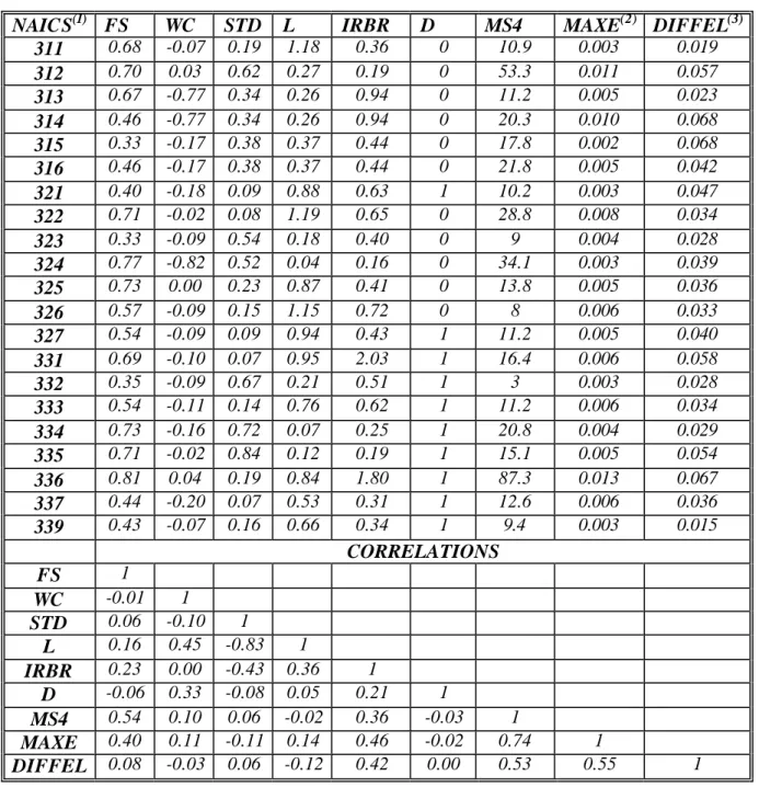
(19) of value added accounted for by the four largest Þrms in each of the sectors in 1997.14 We also considered other variables to account for the inßuence of factors related to the interest rate and the credit channels of monetary transmission. A brief explanation of these variables follows.15 To measure the importance of the traditional interest-rate channel, we consider a durability dummy, D, that takes the value 1 when the industry produces a durable good and zero otherwise.16 We include this variable because it may capture demand sensitivity to changes in interest rates. The idea is that the consumption of non-durable goods may be expected to ßuctuate less. To account for the importance of the potential credit limitations we consider several indicators. The Þrst variable is the short term debt ratio, ST D, computed as the ratio of short term debt to total debt. In addition we use a measure of Þrm size, F S (number of employees in Þrms with more than 500 employees over total number of employees); Þnancial leverage, L, (total debt over shareholders’ funds); and the interest burden, IRBR, (interest rate payments divided over operating proÞts). We use F S and L as proxies for the borrowing capacity of Þrms. It is expected that smaller Þrms and Þrms with lower leverage are more likely to face Þnancial constraints (for a given level of interest burden).17 Finally, the interest burden indicator provides a measure of how production cost changes after an interest rate shock and also a measure of deterioration of credit worthiness.18 Correlations of these indicators with the measures of impact of monetary policy are shown in table 1.. [INSERT TABLE 1] The Þrst thing to notice is that the correlations suggest that maximum elasticity is positively correlated to our index of market concentration. This result is compatible with the intuition 14. Other measures of market concentration, described in section 4, are highly correlated with MS4 and the results. of the analysis do not change when they are used. We don’t use the HerÞndal Index because this is not available for the Transportation Equipment sector. 15. These are the same variables used by Dedola and Lippi [9] to account for their sectoral responses for different. OECD countries. The only differences is that we use a measure of Þrm size which is slightly different from theirs: this difference has no consequence for our results. Also note that given the different classiÞcation between sectors, our durability dummy is not directly comparable to theirs. 16. Industries producing durable goods are Wood Products; Non Mineral Metallic Products; Primary Metal;. Fabricated Metal Products; Machinery; Computer and Electronic Products; Electrical Equipment, Appliance and Components; Transportation Equipment; Furniture and Related Products and Miscellaneous. 17. Gertler and Gilchrist [14] and Fisher [12] argue that Þrm size and leverage respectively are good indicators for. a Þrm’s Þnancial contraints. 18. Our measure of Þrm size comes from the 2001 Employment Size of Firms dataset, available from the Office of. Advocacy for the US Small Business Bureau while the other measures are the 2001 averages from the Quarterly Financial Reports of the US Census Bureau.. 18.

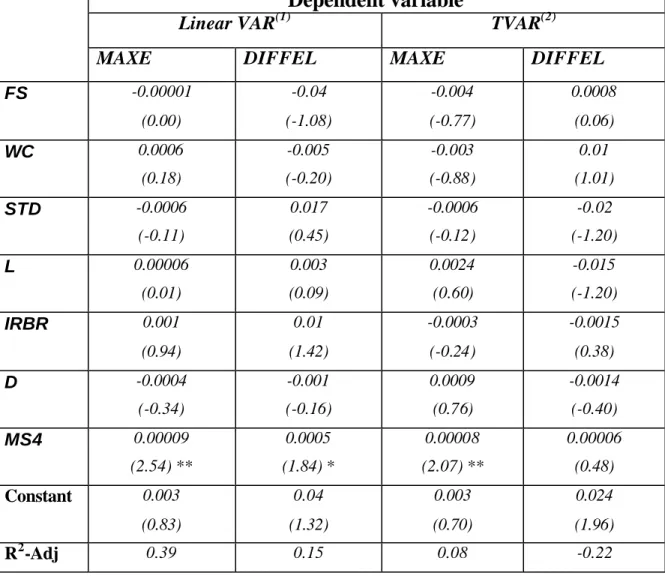
(20) provided by proposition 3. We should note that for robusteness we checked the correlation between our index of market concentration and the elasticity of the responses after eight months and found this to be equal to 63%, which is still quite large. However, we Þnd the maximum elasticity measure to be a more reliable indicator since it is independent to the timing of the reactions, which is different across sectors. We can go further than this by observing the marginal effect of market concentration on reactions while using the other controls described above. This is especially important in this context as there are, for example, important correlations between our measure of market concentration and the size of Þrms and between short term debt and leverage. In order to deal with this issue, we run a simple OLS regression in which MAXE is related to MS4 and the other controls. Estimations are exhibited in table 2 below.. [INSERT TABLE 2] The regression results show that our measure of market share is the only signiÞcant variable at the 5% level. SpeciÞcally, even when we control for a number of indicators related to the interest rate and credit channels and to durability, more concentrated sectors react more intensively and faster to monetary shocks. Further if we adopt a stepwise procedure and remove variable in reverse order of signiÞcance, market share remains as the only important variable in the regression. When we look at the industrial reactions in periods of low uncertainty, we observe from Þgures 2-6 that in those periods the responses of most of the sectors are weaker, compatibly with proposition 5. As further conÞrmation, in table 1, for each sector we compute the sum of the per-period differences in each sector for the two regimes (DIF F EL). This variable is positive for all sectors and highly correlated with our measure of market concentration.19 In table 2, we regressed DIF F EL with MS4 and our usual controls and again Þnd that MS4 is the only variable at the 10% signiÞcance level. In the VAR speciÞcation where p = 2, most of the results remain. In particular, we still Þnd that MS4 is the most important explanatory variable for MAXE and that reactions are stronger in the high uncertainty regime. However, the correlation between MS4 and DIF F EL, while still positive, (18%) is considerably weaker. Our Þnal robustness check involves our TVAR speciÞcation, where again we choose p = 4 in order to compare with our main VAR models. Also, as described in section , we considered three different measures of uncertainty. We report our results for the the rolling standard deviation of the natural logarithm of annual growth of the industrial production index but similar results are 19. We also computed the difference between the maximum elasticity in periods of high uncertainty and the. maximum elasticity in periods of low uncertainty and found analogous results.. 19.

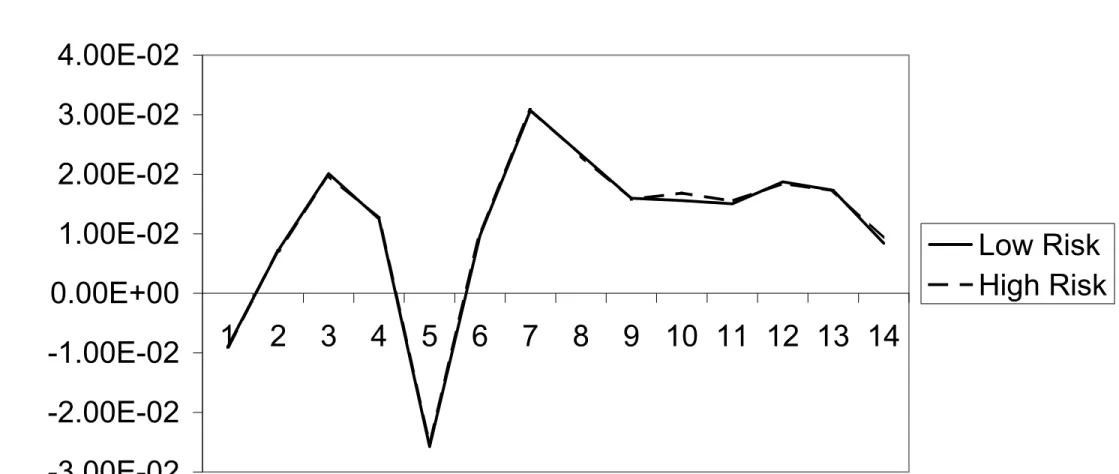
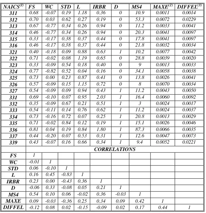
(21) obtained with the other measures.20 In Þgure 7, we show the sum of the response functions for all sectors.. [INSERT FIGURE 7 HERE] Sector by sector responses are not reported but, compatibly with result in Þgure 7, they show that reactions are qualitatively similar to the equivalent VAR responses, with one important difference. Here, the distance between the reactions in the high and low uncertainty regimes are much smaller. This is not entirely surprising since in the simulations we have allowed the model to switch from one regime to the another after a shock, in response to changes in the level of uncertainty. Thus, reactions can “average out” between the two regimes. In table 3, we repeat our correlation for our TVAR model and show that, compatibly with the discussion above, M S4 has a 42% correlation with MAXE while the correlation between MS4 and DIF F EL is positive (17%) but not very high.. [INSERT TABLE 3 HERE] To summarize these Þndings, we can argue that our analysis provides strong evidence for the importance of market structure in the monetary transmission mechanism. It is particularly interesting to note that market structure seems to be a more important factor than other factors that have been put forward by the literature as important determinants of the effects of monetary policy. With respect to the role played by macroeconomic uncertainty, the evidence is less clear. According to our theory, high uncertainty should enhance the effects of market concentration on monetary policy. This prediction is conÞrmed by our VAR model with 4 lags but not by our TVAR approach nor by the VAR model with two lags. Thus, these latter results still await further investigation.. 7. Conclusions This paper documents and analyses sectoral reactions of output to interest rate shocks for 21 manufacturing sectors in the US. To motivate the paper, we have presented a simple model which focuses on the interaction of Þrms’ production and investment decisions when entry is restricted and in the presence of uncertainty about future levels of demand. The model generated two main implications for the empirical analysis: 1) the level of market concentration plays a key role in 20. Note that in the appendix we discuss a linearity test and argue that the null assumption of linearity is rejected. in all cases.. 20.

(22) explaining the heterogeneity of Þrms’ reactions to interest rate shocks; and 2) future uncertainty strengthens today’s output reactions to interest rate shocks. The empirical analysis uses structural VAR and TVAR models to estimate output reactions to monetary shocks for 3 digit NAICS manufacturing industries in the USA and for the 19722003 period. Our results indicate that, among a number of indicators that account for potential restrictions in the credit market and for demand sensitivity, market share is the most important factor in explaining the heterogeneity of output responses. More speciÞcally, we Þnd that, compatibly with our theory, output responses to interest shocks are stronger and faster in highly concentrated sectors. We also Þnd some evidence that reactions are stronger in high uncertainty periods The results suggest a number of policy implications. For example, to the entent that Þnancial reforms in the early 80s have removed the possibility for future periods of high uncertainty, as is claimed by for example, Blanchard and Simon [5] or Stock and Watson [34], this has had a dampening effect on the intensity of output growth reactions to monetary policy. More importantly, in a large, relatively closed economy like the United States, our results suggest that market structure will play an important role in explaining the heterogeneity of the responses to monetary policy, and this more so that some of the other factors that have been put forward in the previous literature. The entent to which these results carry over to other, more open economies, remains to be investigated.. 21.

(23) References [1] Abel, A. and Eberly, J., 1999, “The Effects of Irreversibility and Uncertainty on Capital Accumulation”, Journal of Monetary Economics, 44, 339-377. [2] Atanasova, C., 2003, “Credit Market Imperfections and Business Cycle Dynamics: A Nonlinear Approach”, Studies in Nonlinear Dynamics and Econometrics, 7:4, Article 5. [3] Bernanke, B., Gertler, M., and Gilchrist, S., 1996, “The Financial Accelerator and the Flight to Quality”, Review of Economics and Statistics, 78:1, 1-15. [4] Bernanke. B, and M. Gertler, 1995. “Inside the Black Box: the Credit Channel of Monetary Policy Transmission”, The Journal of Economic Perspectives, 9, 27-48. [5] Blanchard, O. and J. Simon, 2001. “The Long and Large Decline in US Output Volatility”, Brookings Papers on Economic Activity, 1, 135-164. [6] Caballero, R. and R. Pindyck, 1996. “Uncertainty, Investment and Industry Evolution”, International Economic Review, 37:3, 641-662 [7] Christiano, L., Eichenbaum, M and C, Evans 1999. “Monetary Shock: What We Have Learned and to What End” in Handbook of macroeconomics, Volume A, Editors: John B.Taylor, Michael Woodford, North-Holland, 65-148. [8] Dale, S. and A.G. Haldane. 1995. “Interest Rates and the Channels of Monetary Transmission: Some Sectoral Estimates”, European Economic Review, 39, 1611-26. [9] Dedola, L. and F. Lippi, 2000,. “The Monetary Transmission Mechanism: Evidence from Industries of Five OECD Countries”, forthcoming, European Economic Review. [10] Dixit, A., 1991, “Irreversible Investment with Price Ceilings”, Journal of Political Economy, 99:3, 541-557. [11] Dixit, A. and R.S. Pindyck, 1994, Investment and Uncertainty. Princeton University Press. Princeton (New Jersey). [12] Fisher, J., 1999, “Credit Market Imperfections and the Heterogenous Response of Firms to Monetary Shocks”, Journal of Money, Credit and Banking, 31, 187-211. [13] Gertler, M. and S. Gilchrist, 1993, “The Role of Credit Market Imperfections in the Transmission of Monetary Policy: Arguments and Evidence”, Scandinavian Journal of Economics, 95, 43-64. [14] Gertler, M. and S. Gilchrist, 1994, “Monetary Policy, Business Cycles and the Behaviour of Small Manufacturing Firms”, Quarterly Journal of Economics, 109, 309-340. 22.

(24) [15] Hansen, B., 1996, “Inference When a Nuisance Parameter is Not IdentiÞed Under the Null Hypothesis”, Econometrica, 64, 413-30. [16] Hansen, B., 1997, “Inference in TAR Models”, Studies in Nonlinear Dynamics and Econometrics, 2:1, Article 1. [17] Hubbard, R., 1998, “Capital-Market Imperfections and Investment”, Journal of Economic Literature, 36, 193-225. [18] Huizinga, J., 1993, “Inßation Uncertainty, Relative Price Uncertainty, and Investment in US Manufacturing”, Journal of Money, Credit and Banking, 25, 521-54. [19] Kaplan, S., and Zingales, L., 1997, “Do Investment-Cash Flow Sensitivities Provide Useful Measures of Financing Constraints?”, Quarterly Journal of Economics, 112, 169-215. [20] Karras, G., 1996 “Are the Output Effects of Monetary Policy Asymmetric? Evidence From a Sample of European Countries”, Oxford Bulletin of Economics and Statistics, 58, 267-278. [21] Kiyotaki, N. and Moore, J., 1997, “Credit Cycles”, Journal of Political Economy, 105, 21148. [22] Kiyotaki, N. 1998. “Credit and Business Cycles”, The Japanese Economic Review, 49, 1, 18-35. [23] Koop, G., Pesaran, M.H. and Potter, S.M. 1996. “Impulse Response Analysis in Nonlinear Multivariate Models”, Journal of Econometrics, 74, 119-147. [24] Leahy, J., 1993, “Investment in Competitive Equilibrium: The Optimality of Myopic Behavior”, Quarterly Journal of Economics, 108, 1105-1133. [25] Leahy, J., and T.Whited, 1996, “The Effects of Uncertainty on Investment: Some Stylized Facts”, Journal of Money, Credit and Banking, 28, 64-83. [26] Levitan, R. and M. Shubik, 1972 “Price Duopoly and Capacity Constraints”, International Economic Review, 13, 111-122. [27] McDonald, R. and D. Siegel, 1986, “The Value of Waiting to Invest”, Quarterly Journal of Economics, 101, 707-727. [28] Pindyck, R., 1986, “Capital Risk and Models of Investment Behaviour”, MIT, Sloan School of Management Working Paper No.1819. [29] Price, S., 1996, “Aggregate Uncertainty, Investment and Asymmetric Adjustment in the UK Manufacturing Sector”, Applied Economics, 28, 1369-79.. 23.

(25) [30] Seade, J, 1980, “On the Effects of Entry”, Econometrica, 48, 479-490. [31] Shiller, R.J., 1989, Market Volatility, Cambridge MA: MIT Press. [32] Sims, C.A., 1980, “Macroeconomics and reality”, Econometrica 48, 1-48. [33] Sims, C.A., 1992. “Interpreting the Macroeconomic Time-series Facts: the Effects of Monetary Policy”. European Economic Review, 36, 975-1011. [34] Stock, J. and M. Watson, 2002, “Has the Business Cycle Changed and Why?”, NBER Macroeconomics Annual, 159-218. [35] Tong, H. 1983. “Threshold Models in Nonlinear Time Series Analysis”, Lecture Notes in Statistics, 21. Berlin: Springer. [36] Tong, H, 1990, Non-Linear Time Series. A Dynamical System Approach, Oxford: Oxford University Press. [37] Tsay, R., 1998, “Testing and Modelling Multivariate Threshold Models”, Journal of the American Statistical Association, 93, 1188-202. [38] Vives, X, 1986 “Rationing Rules and Bertrand-Edgeworth Equilibria in Large Markets”, Economic Letters, 21, 113-116. [39] Weise, C.L. 1999 “The Asymmetric Effects of Monetary Policy: A Nonlinear Vector Autoregression Approach”, Journal of Money, Credit and Banking, 31:1, 85-108. [40] Wright, S., 2002, “Monetary Policy, Nominal Interest Rate, a Long-Horizon Inßation Uncertainty”, Scottish Journal of Political Economy, 40, 61-90.. 24.

(26) Appendix A: Sketch of Proof for Lemma 1 In what follows, since both periods are exactly symmetric, we drop the superscript t. If a ≤ n − 1. then n − 1 Þrms with capacity equal to one can satisfy all market demand at price zero. Thus, we have a Bertand equilibrium at that price.. Now, suppose that a ≥ n + 1. In this case, producers sell all their capacity at price a − n. If. any producer sets a price below that, then they still sell all their capacity but at a lower price. If a producer i chooses a price pi > a − n, the residual demand would be qi = a − pi − (n − 1) so that proÞts would be (a − qi − (n − 1)) qi where the derivative evaluated at qi = 1 becomes a − n − 1 which is non-negative. Hence, there is no incentive to lower quantity (raising prices). This proves that p = a − n is an equilibrium.. To show that it is unique, note that in any putative equilibrium in which all producers set price p < a − n, there is always an opportunity for a producer to charge a higher price and still sell all. the capacity. If all producers sell at a price p > a − n, then each producer would be selling at less than capacity as qi =. a−p n. < 1. But then, by charging p − ε, a producer can guarantee itself. to sell all capacity. There is always an ε small enough such that pqi < (p − ε) . Finally, note that. an equilibrium in which different producers sell at different prices is also not possible. Let pi. be the lowest of such prices. If at that price the producer is capacity constrained, it can always raise the price and be better off unless pi was the monopoly price and the producer supplied all demand at that price. But then any other producer can always undercut this price and make a positive proÞt. Consider now the case in which n − 1 < a < n + 1. There is no equilibrium in pure strategies. but Dasgupta and Maskin [?] show that there must exist a symmetric, mixed strategy equilibrium £ ¤ where the support of the equilibrium price strategy is an interval p, p and the equilibrium dis-. tribution itself is atomless except perhaps at p. To determine the distribution function explicitly,. we proceed as follows. Let pi be the price set by producer i and let l be the number of producers that charge lower prices than pi and s the number of producers that charge exactly pi . Given our rationing scheme, we get that. 1 (a − p − l) s This means that when either of the two boundaries of the support of the equilibrium distribution qi =. is chosen, demand becomes. qi (pi ) =.    . min (1, a − pi ). if.    max (0, min (1, a − pi − (n − 1))) if 25. pi = p pi = p.

(27) Given that all producers play according to F , there is no other producer that plays exactly p, so by choosing this price, producer i gets to sell to all the market or up to capacity, whichever is smaller. Under the same circumstances, if producer i chooses p, it will get the residual demand after all the other producers’ capacity has been exhausted. Clearly, this residual demand could be zero. It is easy to see that given the residual demand at p described above, p itself must be equal to the monopoly price set with respect to this residual demand whenever the latter is positive. Thus let p=. 1 (a − (n − 1)) = arg max [p (a − p − (n − 1))] p 2. We have that (a − p − (n − 1)) > 0 because a > n−1 and (a − p − (n − 1)) < 1 because a < n+1. Thus, qi (p) = p while Eπi (p) = p2 . This, together with the fact that proÞts are constant for any £ ¤ p in p, p also implies that p = Eπi (p) = p2 because at p the producer would sell to capacity. £ ¤ Following on this logic, expected sales for any price pi in p, p can be written as ³ ´ EF (qi ) = 1 − F (n−1) (pi ) + (a − pi − (n − 1)) F (n−1) (pi ). where F (n−1) (pi ) is the probability that in equilibrium producer i will be charging the highest. price.21 But pi EF (qi ) has to be equal to Eπi (p) = p which, solving for F (pi ) gives ·. pi − p F (pi ) = pi (pi + n − a)). ¸. 1 n−1. as desired ¤ 21. Since the distribution is atomless except at the highest price and all players sell their capacities, the probability. of ties is zero.. 26.

(28) Appendix B: TVAR Estimation Our TVAR estimation is based on a recent paper by Atanasova [2]. Atanasova extends the procedure in Hansen [15] and [16] for the estimation of TVAR models in order to describe asymmetries in the monetary policy transmission mechanism.. B.1. TVAR Model In our TVAR model, regimes are determined by the position of a variable that indicates the degree of macroeconomic uncertainty relatively to an endogenous threshold level. Formally, we consider the model . Yt = Φ10 +. p X j=1. . . Φ1j Yt−j  I(ut−1 ≤ γ) + Φ20 +. p X j=1. . Φ2j Yt−j  I(ut−1 > γ) + at. (B.1). where p is the number of lags, Yt is a (5x1) vector of endogenous variables, including ∆Rt , ∆ot , πt , ∆it and changes in “Industrial Production” in those sectors for which we wish to estimate the reaction. In addition, Φ1j and Φ2j are polynomial matrices, I(.) is an indicator function, at is a (5x1) vector of zero mean, serially uncorrelated disturbances while ut−1 is a scalar measuring the degree of macroeconomic uncertainty in the most recent period, (t − 1). γ is the endogenous threshold parameter. A brief discussion of the procedure used to estimate B.1 follows.. Given observations {Yt , ut−1 } for t = p + 1, ..., T, the model is estimated by conditional least. squares. More speciÞcally, for each of our observations of macroeconomic uncertainty ut−1 we. estimate the parameters in expression B.1 by ordinary least squares, using ut−1 = γ. For each regression, we compute the sum of square errors σ b2T (γ). Then, the LS estimate of γ is computed as. b2T (γ) γ b = arg min σ γ.Γn. (B.2). £ ¤ £ ¤ where Γn = {ut−1 }Tt=1 ∩ γ, γ . The restriction that only values in γ, γ are accepted is imposed in order to guarantee that we have a sufficient number of observations for both the high and low uncertainty cases.22 Theorem 3 in Tsay [37] shows that the conditional least square estimates are strongly consistent as the sample size increases. Just as in the VAR models in the main text, we set p = 4. Correlograms of the residuals for this speciÞcation do not show any known structure. Once the model is estimated, we also tested whether or not the model in B.1 is linear. The null hypothesis was H0 : Φ1j = Φ2j for 22. In order to identify the system, we select γ and γ in such a way that the smallest 30% and largest 30% values. of ut−1 are removed.. 27.

(29) j = 1, ..., p. The Wald Statistic for this test does not follow a standard distribution, because γ is not identiÞed under the null hypothesis. Thus, we obtain the critical values by Monte Carlo simulation, using a procedure described in Atanasova [2] (page 7). The null (linearity) can be rejected at the conventional levels for all cases.23. B.2. Estimation of Impulse Response Functions in Threshold Models In order to estimate impulse response functions, a structural form of model B.1 is deÞned by     p p X X A1j Xt−j  I(ut−1 ≤ γ) +  A2j Xt−j  I(ut−1 > γ) + εt A0 Yt =  j=1. (B.3). j=1. −1 2 1 2 where Φ1j = A−1 0 Aj ; Φj = A0 Aj and fundamental shocks εt are required to be standardized and 0. orthogonal so that Eεt εt = I. Model B.3 is identiÞed by imposing a recursiveness assumption in the same way as with the VAR models. Once model B.3 is identiÞed, it can be used to estimate impulse responses to fundamental shocks. Since the model is nonlinear, these functions cannot be obtained analytically and they are not symmetric and independent of the history of the process. The impact of the fundamental shocks may depend on the sign and size of the shock as well as on the history of the process. Koop et al. [23] discuss this issue and propose a methodology to estimate impulse response functions in nonlinear models based on Monte Carlo simulations of the system. This procedure was used in our analysis to estimate the effect of interest shocks on the output for our 21 US manufacturing sectors. The next section discusses the procedure in detail.24. B.3. Estimation of the Impulse Response Function The objective is to compute sectoral output reactions to monetary shocks. • The parameters for the nonlinear system 5.1 are estimated with the methodology described in subsection section 5.1. • We picked a starting value wt−1 for the simulation of the system. • We picked r samples of 5-dimensional shocks. This is done by using the inverse of a Cholesky factorization of the estimated covariance matrix. This transforms the residuals of the. nonlinear model in contemporaneous independent shocks (εt ). That is, b εt = P −1b at , where. b at are the residuals of the model and P is the lower triangular Cholesky decomposition of. the residuals. In order to recover the sample of residuals, we drew r unordered collections. 23. Details are available upon request.. 24. Gauss programs of all our procedures are available from the authors upon request.. 28.

No results found