PRACTICAL METHODS FOR CRITICAL LOAD DETERMINATION AND STABILITY EVALUATION OF STEEL STRUCTURES
By
PEDRO FERNANDEZ
B.S., Instituto Tecnologico y de Estudios Superiores de Occidente, 1992
A Thesis submitted to the
Faculty of the of the Graduate School of the University of Colorado in partial fulfillment
Of the requirements for the degree of Master of Science
Civil Engineering 2013
This thesis for the Master of Science degree by Pedro Fernandez
has been approved for the Civil Engineering Program
by
Fredrick Rutz, Chair
Kevin Rens
Chengyu Li
Fernandez, Pedro. (M.S., Civil Engineering)
Practical Methods for Critical Load Determination and Stability Evaluation of Steel Structures
Thesis directed by Assistant Professor Fredrick Rutz
ABSTRACT
The critical load of a column, compression member or structure, calculated from a linear elastic analysis of an idealized perfect structure, does not necessary correspond with the load at which instability of a real structure occurs. This calculated critical load does not provide sufficient information to determine when failure, due to instability of the structure as a whole, will occur. To obtain this information it is necessary to consider the initial geometrical imperfections, eccentricities of loading, and the entire nonlinear load deflection behavior of the structure. However, this process in determining the critical load is too cumbersome and time consuming to be used in practical engineering applications.
With today’s computer programs that allow for the analysis of complex structures in which they incorporate advanced analytical techniques such as step-by-step large deformation analysis, buckling analysis, progressive collapse analysis, etc., it is just a natural progression that many structures are now analyzed with these tools.
The goal of this research is to propose a practical methodology for critical load determination and stability evaluation of structures that are difficult or impossible to analyze with conventional hand-calculation methods, (e.g. the
compression cord of a truss pedestrian bridge or a wind girt). The proposed methodology relies on a computer software package that has the ability to perform a second-order analysis taking in consideration end-restraints, reduced flexural stiffness (due to residual stresses in steel or cracked sections in concrete) and initial geometrical imperfections. Further, and importantly, a testing scheme was developed to validate the results from the computer in order to verify the methodology as a practical approach.
The format and content of this abstract are approved. I recommend its publication.
Approved: Fredrick R. Rutz
DEDICATION
I dedicate this work to Mary Lynne, my wife, my parents,
my brother, Coco and Nina
...and in the loving memory of my grandparents
ACKNOWLEDGMENTS
I would like to thank first and foremost Dr. Fredrick Rutz for the support and guidance in completion of this thesis. I would also like to thank Dr. Rens and Dr. Li
for participating on my graduate advisory committee. Lastly, I would like to thank Paul Jones, the artist, who built the test models with so much precision and passion,
TABLE OF CONTENTS CHAPTER
I. INTRODUCTION ... 1
Research Program Objectives ... 4
Outline of Research ... 6
II. A HISTORICAL APPROACH ON STRUCTURAL STABILITY ... 9
Euler ... 9
Effective Length Factors ... 11
Inelastic Buckling Concepts ... 16
Tangent Modulus ... 19 Reduced Modulus ... 21 Shanley Theory ... 22 Amplification Factors ... 23 Braced Frames ... 25 Unbraced Frames ... 28
Column Strength Curves ... 30
Summary of Present State of Knowledge ... 33
III. COLUMN THEORY ... 34
Mechanism of Buckling ... 35
Critical Load Theory ... 37
Euler Buckling Load ... 40
Second Order Effects ... 49
Inelastic Buckling of Structures ... 52
Factors Controlling Column Strength and Behavior ... 54
Material Properties ... 55
Length ... 56
Influence of Support Conditions ... 57
Moment Frames ... 57
Members with Elastic Lateral Restraints ... 61
Influence of Imperfections ... 64
Material Imperfections ... 65
Geometrical Imperfections ... 68
IV. METHODS AND PROCEDURES FOR ANALYSIS AND DESIGN OF STEEL STRUCTURES ... 71
Structural and Stability Analysis ... 71
First-Order Elastic Analysis ... 73
Elastic Buckling Load ... 74
Second-Order Elastic Analysis ... 74
First-Order Inelastic Analysis ... 75
Second-Order Inelastic Analysis ... 76
Design of Compression Members ... 76
Determining Required Strength ... 79
Determining Available Strength ... 80
Combined Forces ... 85
Current Stability Requirements (AISC Specifications) ... 87
The Effective Length Method ... 89
Direct Analysis Method ... 90
Imperfections ... 91
Reduced Flexural and Axial Stiffness ... 92
Advanced Analysis ... 93
Pony Truss Bridges ... 96
V. STABILITY ANALYSIS USING NONLINEAR MATRIX ANALYSIS WITH COMPUTER SOFTWARE ... 99
Matrix Structural Analysis ... 99
Direct Stiffness Method ... 101
Nonlinear Analysis using Matrix Methods ... 102
Computer Software Used ... 105
P-Δ and P-δ ... 106
Modeling Geometrical Imperfections ... 108
Assessment of the Computer Software with Benchmark Problems from Established Theory... 109
VI. A PRACTICAL METHOD FOR CRITICAL LOAD DETERMINATION OF STRUCTURES ... 112
Proposed methodology: Step-by-step process ... 113
VII. COMPUTER SOFTWARE EVALUATION WITH BENCHMARK PROBLEMS ... 116
Benchmark Problem 1... 118
Discussion of Results from Benchmark Problems... 133
VIII. MODEL DEVELOPMENT ... 134
Full-Size Analytical Study ... 135
Experimental Study ... 144 Theoretical Models ... 145 Bridge 1 ... 145 Bridge 2 ... 146 Loading ... 149 Geometric Imperfections ... 150 Procedure ... 151 Test Models ... 152 Test Setup... 155
Load Testing Procedure ... 159
IX. EXPERIMENTAL RESULTS ... 161
Bridge 1 Results ... 164
Theoretical Results... 164
Load Test Results ... 168
Bridge 2 Results ... 177
Theoretical Results... 177
Load Test Results ... 181
X. CONCLUSIONS ... 187
Research Overview ... 187
General Recommendations ... 189 REFERENCES ... 191 APPENDIX 1: TEST MODELS PLANS ... 197
LIST OF FIGURES Figure
1.1 Pony truss bridge (Excelbridge 2012) ... 3
2.1 (a) Cantilever Column, (b) Pinned End Column ... 10
2.2 Effective Column Lengths. (a) Pinned End, (b) Cantilever and (c) Fixed-end .... 12
2.3 Effective Length Factors K for centrally loaded columns (Adapted from Chen 1985) ... 14
2.4 Effective length of a moment frame with joint translation (Adapted from Geschwindner 1994) ... 14
2.5 Effective length factors (Adapted from AISC 2005) ... 16
2.6 Column Critical Stress for various slanderness ratios (L/r) (Adapted Gere 2009) 17 2.7 Stress-strain diagram for typical structural steel in tension (Adapted from Gere 2009) ... 18
2.8 Definition of tangent modulus for nonlinear material (Adapted from Geschwindner 1994) ... 20
2.9 Stress distributions for elastic buckling: (a) tangent modulus theory; (b) reduced modulus theory (Adapted from Geschwindner 1994) ... 22
2.10 Load-deflection behavior for elastic and inelastic buckling (Adapted from Gere 2009) ... 23
2.11 Axial loaded column with equal and opposite end moments (Adapted from Geschwindner 1994) ... 26
2.12 Amplified moment: exact and approximate (Adapted from Geschwindner 1994) ... 27
2.13 Structure second-order effect: sway (Adapted from Geschwindner 1994) ... 28
2.14 Column strength variation (Adapted from Ziemian, 2010) ... 32
3.2 Column Stability (Adapted from Chen 1985) ... 38
3.3 Beam-Column Stability (Adapted from Chen 1985) ... 39
3.4 Pin-ended supported column... 41
3.5 Euler Curve ... 45
3.6 Beam-Column (Adapted from Chen 1985) ... 46
3.7Elastic analysis of initially deformed column (Adapted from Chen 1985) ... 49
3.8 Second-order effects ... 52
3.9 Residual stresses and proportional stress (Chen 1985) ... 54
3.10 Typical stress-strain curves for different steel classifications ... 56
3.11 Theoretical column strength (Gere 2009) ... 57
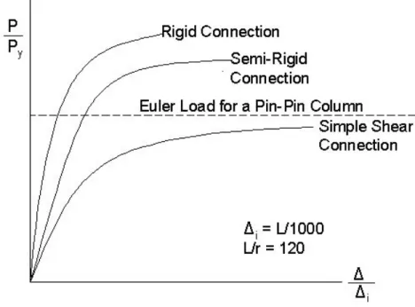
3.12 Typical load-deflection curves for columns with different framing beam connections (Adapted from Ziemian 2010) ... 58
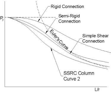
3.13 Column strength curves for members with different framing beam connection (Adapted from Ziemian 2010) ... 59
3.14 Connection flexibility (Adapted from AISC 2005) ... 59
3.15 Pony truss and analogous top chord (Adapted from Ziemian 2010) ... 63
3.16 Influence of imperfections on column behavior (Adapted from ASCE Task Committee 1997) ... 65
3.17 Column curve for structural steels. (a) elastic-perfectly plastic stress-strain relationship; (b) column curve (Adapted from Chen 1985) ... 66
3.18 Lehigh residual stress pattern (Adapted from Surovek 2012) ... 68
4.1 Comparison of load-deflection behavior for different analysis methods (Adapted from Geschwindner 1994) ... 73
4.2 Distinction between effective length and notional load approaches (Adapted from Ziemian 2010). ... 81
4.4 Interaction curve (Adapted from Williams 2011) ... 87
4.5 Lateral U-Frame (Adapted from AASHTO 2009) ... 97
5.1 Schematic representation of incremental-iterative solution procedure. (Ziemian 2011) ... 105
5.2 RISA second-order effects process (Adapted from RISA-3D 2012) ... 107
5.3 Benchmark Problem 1 (AISC 2005) ... 110
5.4 Benchmark Problem 2 (AISC 2005) ... 111
6.1 Error message from RISA-3D that P-Δ is no longer converging ... 115
7.1 Benchmark Problem 1 (AISC 2005) ... 117
7.2 Benchmark Problem 2 (AISC 2005) ... 117
7.3 Benchmark problem 1: a) undeflected shape b) deflected shape ... 121
7.4 Maximum moment values as a function of axial force for benchmark problem 1 (classical solution, Equation 7.2) ... 122
7.5 Maximum deflection values as a function of axial force for benchmark problem 1 (classical solution, Equation 7.3) ... 122
7.6 Benchmark problem 1 node arraignments a) Case 1, one additional node at mid height of the beam-column b) Case 2, two additional nodes at equal distance c) Case 3, three additional nodes at equal distance ... 123
7.7 Maximum moment values as a function of axial force for benchmark problem 1 (classical solution, with one, two and three additional nodes) ... 124
7.8 Maximum deflection values as a function of axial force for benchmark problem 1 classical solution, with one, two and three additional nodes) ... 125
7.9 Benchmark problem 2, a) undeflected shape b) deflected shape ... 127
7.10 Maximum moment values as a function of axial force for benchmark problem 1 (classical solution, Equation 7.5) ... 129
7.11 Maximum deflection values as a function of axial force for benchmark problem 1 (classical solution, Equation 7.6) ... 129
7.12 Benchmark problem 2 node arraignments a) Case 1, no additional node along the height of the beam-column b) Case 2, one additional node at mid height of the
beam-column c) Case 3, two additional nodes at equal distance ... 130
7.13 Maximum moment values as a function of axial force for benchmark problem 2 (classical solution, with zero, one and two additional nodes) ... 131
7.14 Maximum deflection values as a function of axial force for benchmark problem 2 (solution, with zero, one and two additional nodes) ... 132
8.1 Actual 40 foot long pony truss bridge... 137
8.2 Computer model of the 40 foot long bridge (analytical model) ... 137
8.3 Parametric study... 139
8.4 Geometric imperfection ... 140
8.5 Deformed shape at critical load. Slender top chord ... 142
8.6 Deformed shape at critical load. Stiffer compression chord ... 142
8.7 Bridge 1 truss geometry ... 147
8.8 Bridge 1 computer model of truss ... 147
8.9 3D Model of Bridge 1 ... 147
8.10 Bridge 2 truss geometry ... 148
8.11 Bridge 2 computer model of truss ... 148
8.12 3D model of Bridge 2 ... 148
8.13 Load test setup diagram ... 149
8.14 Bridge 1 computer model loading configuration ... 150
8.15 Bridge 2, computer model loading configuration ... 150
8.16 Modeling of geometric imperfections ... 151
8.17 Bridge 1 Computer Model ... 153
8.19 Bridge 2 Computer Model ... 154
8.20 Bridge 2 Test Model ... 154
8.21 Load test setup diagram ... 156
8.22 Load test setup ... 156
8.23 Spreader beam and plates used to uniformly distribute the load on the bridge deck ... 157
8.24 Typical end support configuration and abutments ... 157
8.25 Load cell... 158
8.26 Data collection setup ... 159
8.27 Test setup top view ... 160
9.1 Bridge 1 Naming convention for top chords ... 162
9.2 Bridge 2 Naming convention for the top chords ... 162
9.3 Top chord initial imperfection, Δo (a) Top view of compression chord (b) Cross-section view ... 163
9.4 Bridge 1 Theoretical results ... 167
9.5 Bridge 1 Theoretical and load test results ... 171
9.6 Bridge 1 Deformed shape at failure ... 172
9.7 Bridge 1 Theoretical (fix-ended diagonals) and load test results ... 174
9.8 Deformation of end-diagonal prior to buckling (test model) ... 175
9.9 Deformation of end-diagonal (computer model) at critical load ... 175
9.10 Deformation of end-diagonal at buckling (test model) ... 176
9.11 Deformation of end-diagonal (computer model) at critical load ... 176
9.12 Bridge 2 Theoretical results ... 180
9.14 Deformed shape at 53% of the critical load ... 185
9.15 Deformed shape at 78% of critical load ... 185
9.16 Deformed shape at 91% of the critical load ... 186
LIST OF TABLES Table
8.1Parametric Study of Analytical Models ... 143
9.1 Measured initial imperfections, Δo, of top chords ... 163
9.2 Bridge 1 Theoretical Results: Top chord ratio Δ/Δo ... 166
9.3 Bridge 1 Theoretical Results: Critical load ... 166
9.4 Bridge 1 Theoretical and Load Test Results: Top chord ratio Δ /Δo ... 170
9.5 Bridge 1 Theoretical and Load Test Results: Critical load ... 170
9.6 Bridge 1 Ratio Δ /Δo, theoretical results with fix-ended diagonals ... 173
9.7 Bridge 1 Critical load, theoretical results with fix-ended diagonals ... 173
9.8 Bridge 2 Theoretical Results: Top chord ratio Δ /Δo ... 179
9.9 Bridge 2 Theoretical Results: Critical load ... 179
9.10 Bridge 2 Theoretical and Load Test Results: Top chord ratio Δ /Δo ... 183
CHAPTER I 1INTRODUCTION
A research project on stability cannot start without recognizing the contribution of Euler to the problem of stability when he published his famous Euler’s equation on the elastic stability of columns back in 1744. And even though the research on the stability of structures can be traced back to 264 years ago since Euler’s contribution to column stability, practical solutions are still not available for some types of structures. Stability is one of the most critical limit states for steel structures during construction and during their service life. One of the most difficult challenges in structural stability is determining the critical load under which a structure collapses due to the loss of stability; this is because of the complexity of this phenomenon and the many material properties that are influenced by geometric and material imperfections and material nonlinearity. In addition to the challenges mentioned above, the advancement in industrial processes in hot-rolled members and the use of high strength steel, which provides a competitive design solution to structural weight reduction, has resulted in increase of member slenderness, structural flexibility and therefore more vulnerability to instability.
The method proposed in this research project for the evaluation of the lateral stability of structures, and to determine their critical load at which they become instable is an innovative approach. It enables the prediction of the characteristics of stability of structures by capturing the load-deformation history and the deformed
shape of the structure at the critical load. Such critical information is generally not available through the current stability analysis methods. Although the method is oriented for analysis of 3D structures, and structures that are difficult to analyze with conventional hand-calculation methods, it can be used for any 2D structure.
Lateral stability of steel structures that are difficult to analyze with conventional hand-calculation methods include: columns under axial compression load and biaxial bending in 3D frames, stepped columns, multi-story columns of different lengths and sections, the unbraced compression chord of a wind-girt truss, and the top chord of a pony truss which due to vertical clearance requirements prohibit direct lateral bracing. Pony truss structures, while no longer as common for construction of new highway or rail bridges, are commonly used in applications similar to Figure 1.1 or as walkways and conveyor systems.
The analysis of the compression chord of a pony truss is typically accomplished by treating the chord as a column with elastic supports (Ziemian 2010). This column, with intermediate elastic restraints, will buckle in a number of half-waves depending on the stiffness of the elastic restraints. The deformed shape or buckled shape of the column will fall somewhere between the extreme limits of a half-wave of length equating the length of the chord and a number of half-waves equating the number of spans between the end restraints, that is, the number of panels. From the buckled shape, the effective length of the compression chord can be
used to determine the critical load. The method on how to determine the effective length has long been the focus of the compression chord buckling problem.
Figure 1.1Pony truss bridge
This research will focus primarily on applying the proposed methodology for the determination of the critical load of pony truss bridges. However, it can be used for any other 3D structures, including framed structures. All structural frames in reality are geometrically imperfect, that is, lateral deflection commences as soon as the loads are applied. There are typically two types of geometric imperfections that are taken into consideration for the stability analysis of structures; out-of-straightness, which is a lateral deflection of the column relative to a straight line between its end
points, and column out-of-plumbness, which is lateral displacement of one end of the column relative to the other. In the absence of more accurate information, evaluation of imperfection effects should be based on the permissible fabrication and erection tolerances specified in the appropriate building code.
In the U.S., the initial geometric imperfections are assumed to be equal to the maximum fabrication and erection tolerances permitted by the AISC Code of Standard Practice for Steel Building and Bridge, AISC 303-10 (AISC 2010). For columns and frames, this implies a member out-of-straightness equal to L/1000, where L is the member length brace or framing points, and a frame out-of-plumbness equal to H/500, where H is the story height. For the critical load determination and load-deformation history evaluation in this research project, three imperfections will be considered: L/300, L/450 and L/700.
Research Program Objectives
The goal of this research project is to propose a practical method for stability evaluation and assessment of structures that are difficult or impossible to analyze with conventional hand-calculation methods. The proposed methodology relies on a commercially available computer program in which a second order analysis can be readily accomplished by taking into consideration end-restraints, reduced flexural stiffness, and initial geometrical imperfections or out-of-plumbness. The method can be used for any frame 3D structure or truss. The specific objectives of this research project are:
1. Develop an analytical process that is based on an iterative approach (with the help of a 3D computer program) that would facilitate the determination of the critical load and stability assessment of steel structures that are difficult or impossible to analyze with conventional hand-calculation methods.
2. Investigate the correctness of the computer program to be able to perform a rigorous second order analysis, by using benchmark problems from established theory, which are presented in AISC 360-05.
3. Conduct an analytical investigation, using the proposed approach, to determine the critical load, the effects of initial imperfections, and the characteristics of the failure mode of full size pony truss models. 4. Develop two scaled pony truss bridges based on the results from item
3 that can be load tested with available equipment.
5. Apply the proposed methodology and determine, analytically, the load-deformation history and critical load of the two scaled pony truss bridges developed in item 4.
6. Develop a testing scheme in which two scaled pony truss bridges are load tested. The testing scheme must include means to measure both of
the top chords out of plane deformations and to determine the load at any instant of the load application.
7. Verify the proposed methodology by comparing the results between the computer model results and the results from the testing scheme.
Outline of Research
In general terms, this research project consisted of a literature review, development of a methodology for critical load determination of structures, and a testing scheme to validate the proposed methodology. This thesis is organized in the following manner:
Chapter II presents a historical background on column stability, from Euler’s early work on column stability and elastic critical load to the development of the column strength curves used in today’s column strength equations. This historical background includes an introduction to the concept of equivalent or effective length, a review of different theories that have been used to predict column strength and an introduction on the derivation of the amplification factors.
In Chapter III, the mechanism of buckling is presented along with the derivation of the critical load for an ideal column with pin supports. An introduction to structural stability of beam-columns and second order effects (P-Δ and P-δ) is discussed. In this Chapter, some of the more critical factors that control column
strength and behavior are reviewed. This review focuses on the effects of geometrical and material imperfections.
The determination of member sizes for a structure, in general terms, is a two step process. First, a structural and stability analysis is performed in order to determine the required strength. Second, empirical equations are used to determine the available strength and then compared to the required strength. Chapter IV presents an overview of the different methods for stability analysis, as well as the procedures and requirements for the determination of the available strength in AISC Specifications for Structural Steel Buildings, AISC 360-05 (AISC 2005) and AASHTO LRFD Guide Specifications for the Design of Pedestrian Bridges, (AASHTO 2012).
Because the proposed methodology requires the use of a computer program, Chapter V presents an introduction to the methods of analysis in most computer software packages. Also in this Chapter, an introduction to the capabilities of the computer software package (RISA-3D) is presented as well as a discussion of its ability to perform a rigorous second-order analysis.
In Chapter VI the proposed methodology is presents as a step by step process with the goal of determining the load-deformation history and critical load of a structure. This process addresses the selection of the computer software package, modeling, the incorporation of geometrical imperfections in the model and the determination of the critical load.
However, it is necessary to evaluate the ability of the software package to perform a rigorous second order analysis. Given in Chapter VII are the results from the benchmark problems used for the evaluation of RISA-3D. Furthermore, in this chapter, a discussion is given on the assessment of the P-δ capabilities of the program.
The development of the testing scheme is given in Chapter VIII and the results are presented in Chapter IX. Conclusions of the current research and recommendations are presented in Chapter X.
CHAPTER II
2A HISTORICAL APPROACH ON STRUCTURAL STABILITY Euler
Any work on structural stability cannot start without a discussion on Leonard Euler (1707-1783), for many, Euler is considered the greatest mathematician of all time (Gere 2009). Euler made great contributions to the field of mathematics, namely, trigonometry, differential and integral calculus, infinite series, analytic geometry, differential equations, and many other subjects (Gere 2009). However, with regard to applied mechanics, Euler made one of the most important contributions to structural engineering concerning with elastic stability of structures, and which is still subject of many studies after almost 270 years: the buckling of columns. He was the first to derive the formula for the critical buckling load of an ideal, slender column.
Euler’s work was published in 1744 under the title “Methodus inveniendi lineas curvas maximi minimive proprietate gaudentes”. His original work consisted on determining the buckling load of a cantilever column that was fixed at the bottom and free at the top as shown in Figure 2.1(a) (Timoshenko 1983).
Figure 2.1(a) Cantilever Column, (b) Pinned End Column
In this case, Figure 2.1(a), Euler shows that the equation of the elastic curve can be readily be solved and that the load at which the buckling occurs is given by Equation 2.1 2 2 4 C P l (2.1)
Later on, Euler expanded his work on columns to include other restraint conditions, and determined the buckling load for a column with pinned supports, Figure 2.1(b) as being 2 2 C P l (2.2)
In his work, Euler did not discuss the physical significance of the constant C which he calls the “absolute elasticity”, merely stating that it depends on the elastic properties of the material (Timoshenko 1983). One can conclude that this constant is the flexural stiffness of the column, EI. Euler was the first to recognize that columns could fail through bending rather than crushing. In his work he states:
Therefore, unless the load P to be borne be greater than C2 4l2 there will be absolutely no fear of bending; on the other hand, if the weight P be greater, the column will be unable to resist bending. Now when the elasticity of the column and likewise its thickness remain the same, the weight P which it can carry without danger will be inversely proportional to the square of the height of the column; and a column twice as high will be able to bear only one fourth of the load (Timoshenko, 1983).
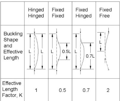
Effective Length Factors
The Euler buckling load equation gives the critical load at which a pin-supported column will buckle, Figure 2.2(a). The critical load for columns with various support conditions, other than a pin-pin support, can be related to this column through the concept of an “effective length”. For example, Figure 2.2(b)a fixed-end column buckles at 4 times the load for a pinned column, and because the Euler buckling load is directly proportional to the inverse square of the length, the effective length of a fixed-end column is one half of that of the same member with pinned ends. At the same time, Figure 2.2(c), a column that is fixed at the base and free at the top will have an effective length of 2L and will buckle at a quarter the load of the pinned-end column.
Figure 2.2 Effective Column Lengths. (a) Pinned End, (b) Cantilever and (c) Fixed-end
Because the effective length, Le, for any column is the length of the equivalent
pinned-end column, then, the general equation for critical loads, for any column with supports other than pin-pin, can be written as
2 2 2 2 e EI EI P L Kl (2.3)Where K is the effective length factor and is often included in design formulas for columns. That is, the Euler buckling load formula can be used to obtain the critical load of a column with different end conditions provided the correct effective length of the column is known, illustrated in Figure 2.3.
In simplified terms the concept is merely a method of mathematically reducing the problem of evaluating the critical stress for columns in structures to that of equivalent pinned-end brace columns (Yura 1971).
So far columns with ideal boundary conditions have been discussed; however, the effective length concept is equally valid for any other set of boundary conditions not included in Figure 2.3, except that the determination for the effective length factor is not as simple or straightforward as in Figure 2.3.
For example, in the case of a column that is part of a moment frame, the effective length factor is a function of the stiffness of the beams and columns that frame into the joint. Columns or compression members can be classified based on the type of frame that they form a part. Columns that don’t participate in the lateral stability of the structure are considered to be braced against sway. A braced frame is one for which sidesway or joint translation is prevented by means of bracing, shear walls or lateral support from adjoining structures. An unbraced frame depends on the stiffness of its members and the rotational rigidity of the joints between the frame members to prevent lateral buckling as shown in Figure 2.4. Theoretical mathematical analysis may be used to determine effective lengths; however, such procedures are typically too lengthy and unpractical for the average designers. Such methods include trial and error procedures with buckling equations.
Figure 2.3 Effective Length Factors K for centrally loaded columns (Adapted from Chen 1985)
Figure 2.4 Effective length of a moment frame with joint translation (Adapted from Geschwindner 1994)
For normal design situations, it is impractical to carry out a detailed analysis for the determination of buckling strength and effective length. Since the introduction of the effective length concept in the AISC specifications for the first time in 1961 (AISC 1961), several procedures have been proposed for a more direct determination of the buckling capacity and effective length of columns in most civil engineering structures (Shanmugam 1995). The most common method for obtaining the effective length of a column or compression member and to account for the effects of the connected members is to employ the alignment charts or nomographs, originally developed by Julian and Lawrence (McCormac 2008). The alignment charts were developed from a slope-deflection analysis of a frame including the effect of column loads (McCormac 2008).
Values of K for certain idealized end conditions are given in Figure 2.5. The values of K for columns in frames, depend on the flexural rigidity of adjoining members and the manner in which sidesway is resisted. The values given in Figure 2.5 are based on the assumption that all columns in a frame will reach their individual critical loads simultaneously. In certain cases, the effective length factors are not applied correctly given that the underlying assumptions of the method do not apply. The method involves a number of major assumptions which are summarized in section C2.2b of the Commentary of the AISC Specification (AISC 2005). Some of the most significant assumptions are: members are assumed to behave elastically, all
columns buckle simultaneously, all members are prismatic and the structure is symmetric (AISC 2005).
Figure 2.5 Effective length factors (Adapted from AISC 2005) Inelastic Buckling Concepts
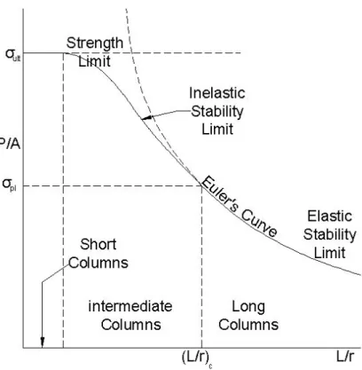
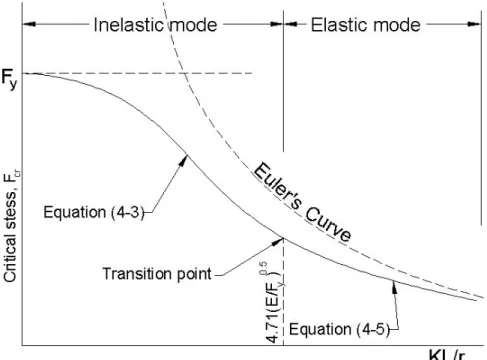
Figure 2.6 shows the theoretical stability behavior of columns as a function of the average compressive strength, P/A versus the slenderness ratio, l/r. From this figure and depending on the type of failure, columns can be classified as short columns, intermediate columns, and long columns. Short or stocky columns fail by crushing while very long columns fail by elastic buckling as described by Euler’s
critical load equation. Euler determined that the critical load for a slender column does not necessary correspond to the crushing strength, but a lower values which is a function of the length of the column and the flexural rigidity as discussed earlier. However, Euler’s critical load for elastic buckling is valid only for relative long columns where the stress in the column is below the proportional limit (Gere 2009).
Figure 2.6Column Critical Stress for various slanderness ratios (L/r) (Adapted Gere 2009)
Many practical columns are in a range of slenderness where at buckling, portions of the column are no longer linearly elastic, and thus one of the fundamental assumptions of the Euler column theory is violated due to a reduction in the stiffness of the column. This degradation of the stiffness may be the result of material
nonlinearity or it may be due to partial yielding of the cross section at certain points where compressive stresses pre-exists due to residual stress (Ziemian 2010). This range is considered as the range of the intermediate columns, thus, intermediate columns fail by inelastic buckling. For columns of intermediate length, the stress in the column will reach the proportional limit before buckling begins. The proportional limit is the limit at which not only the modulus of elasticity or the ratio of stress-strain is linear but also proportional, this can be seen in Figure 2.7. Various theories have been developed to account for this type of behavior in which columns are considered to be in the inelastic range, some of the theories are presented below.
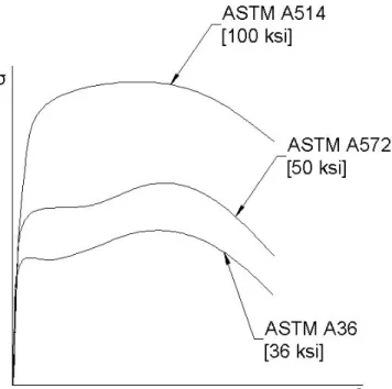
Figure 2.7 Stress-strain diagram for typical structural steel in tension (Adapted from Gere 2009)
Tangent Modulus
In the late 19th century, independent research work done by Engesser and Considère recognized the shortcomings of the Euler theory, in which Euler’s buckling load was based on an elastic material response (Geschwindner 1994). During that time it was already known that various materials exhibited nonlinear characteristics. Engesser developed a theory in which he assumed that the modulus of elasticity at the instant of buckling was equal to the slope of the material stress-strain curve at the level of the buckling stress. In other words, if the load on a column is increased so that the stress is beyond the proportional limit of the material, and this increase in load is such that a small increase in stress occurs, the relationship between the increment of stress and the corresponding increment of strain is given by the slope of the stress-strain curve at point A in Figure 2.8. This slope, which is equal to the slope of the tangent line at A, is called the tangent modulus and is designated by ET,
(Geschwindner 1994) thus, T d E d (2.4)
Engesser rationalized that the fibers in tension (unloading fibers) and the fibers in compression (loading fibers), both, would behave according to the tangent modulus as shown in Figure 2.9(a). Therefore, the buckling load of a column corresponds to the load defined as the tangent modulus load. The buckling load can
then be computed from the Euler buckling expression by substituting the modulus of elasticity with the tangent modulus (Geschwindner 1994).
2 2 T T E I P l (2.5)Figure 2.8 Definition of tangent modulus for nonlinear material (Adapted from Geschwindner 1994)
Because the tangent modulus, ET, varies with the compressive stress, σ = P/A,
the tangent modulus load is obtained by an iterative procedure. From Figure 2.9(a) one can think of the tangent modulus as the average modulus of elasticity of the complete cross section. Some of the fibers will be in the elastic range and others will be in the inelastic range, in other words, some fibers are responding elastically in accordance with the full modulus of elasticity, E, while other respond with a modulus of zero (Geschwindner 1994).
Reduced Modulus
The reduced modulus theory is also known as the double modulus, Er. When a
column bends under loading, in addition to the axial load, bending stresses are added to the compressive stress, P/A due to the axial load. These additional stresses are compression on the concave side and tension on the opposite side of the column. By adding the bending stresses to the axial stresses, it can be seen that on the concave side the stresses in compression are larger than the stresses in tension. Therefore, it can be assumed that on the concave side, the material follows the tangent modulus, Figure 2.9(b) and in the convex side the material follows the unloading line shown in Figure 2.8.
One can think as if this column were made of two different materials (Gere 2009). As in the tangent modulus method, the critical load can be found by replacing the modulus of elasticity, in the Euler equation, by the reduced modulus or double modulus. However, the reduced modulus theory is difficult to use in practice because Er depends not only on the shape of the cross section of the column but the stress
strain curve of that specific column. This means it needs to be evaluated for every different column section type (Gere 2009).
Figure 2.9 Stress distributions for elastic buckling: (a) tangent modulus theory; (b) reduced modulus theory (Adapted from Geschwindner 1994)
Shanley Theory
Tests conducted by von Karman and others over many years (Johnston 1981) have demonstrated that actual buckling loads tend to more closely follow the loads predicted by the tangent modulus equation than those from the reduced modulus equation. In 1947, an American aeronautical-engineering professor F.R. Shanley demonstrated that there would be no stress reversal in the cross section as the column reached the tangent modulus load because the initial deflection at this point was infinitesimal. Shanley proved that the tangent modulus load was the largest load at which the column will remain straight (Geschwindner 1994). Once the load exceeded the tangent modulus load, there would be a stress reversal and elastic unloading would take place and the load carrying capacity is then predicted by the reduced
modulus (Geschwindner 1994). In other words, a perfect inelastic column will begin to deflect laterally when P = PT and P < Pmax < PR, illustrated in Figure 2.10.
Figure 2.10 Load-deflection behavior for elastic and inelastic buckling (Adapted from Gere 2009)
Amplification Factors
Second order effects are the direct result of structural deformations. In order to account for these secondary effects, a nonlinear or second order analysis must be carried out that takes into account equilibrium on the deformed shape of the structure, rather than on the original undeformed shape as is in the case of the traditional classical methods of analysis. An alternate approach for this more rigorous and complex method of analysis, is to determine the secondary effects by amplifying the moments and forces from a first order elastic analysis. The concept of moment
magnification, to account for secondary effects, was introduced in the AISC Specifications in 1961 by including the following expression (AISC 1961):
1 ' m a e C f F (2.6)
for the determination of combined stresses in the following equation
1.0 1 ' a m b a a b e f C f F f F F (2.7)
The commentary to the AISC Specification of 1961 explains the significance of the new term:
The bending stress at any cross section subject to lateral displacement must be amplified by the factor
1 ' m a e C f F (2.8)
it recognizes the fact that such displacement, caused by applied moment, generates a secondary moment equal to the product of the resulting eccentricity and the applied axial load, which is not reflected in the computed stress, fb (AISC 1961).
There are two different magnification factors to account for the secondary effects; one magnification factor is used for columns that are part of a braced frame and a second magnification factor for columns that are part of an unbranced frame. A frame is considered braced if a system, such as shear walls or diagonal braces, serves
to resist the lateral loads and to stabilize the frame under gravity loads. In a braced frame the moments in the column due to the gravity loads are determined through a first order elastic analysis, and the additional moments resulting from the deformation along the column length will be determined through the application of an amplification factor.
Unbraced frames depend on the stiffness of the beams and columns for lateral stability under gravity loads and combined gravity and lateral loads. Unlike braced frames, discussed earlier, there is no supplementary structure to provide lateral stability. Columns that form part of an unbraced frame are subjected to both axial forces and bending moments and will experience lateral translation. The latter will cause an additional second order effect to the one discussed earlier. This second order effect is the result from the sway or lateral displacement of the frame.
Braced Frames
In his paper titled “A Practical Method of Second Order Analysis”, LeMessurier provides the full derivation of the amplification factors for both braced frames and unbraced frames (LeMessurieer 1976). A summary of the derivation is presented below.
Consider the column in Figure 2.11, the maximum moment at mid height of the column is given by equation 2.9
max
Figure 2.11 Axial loaded column with equal and opposite end moments (Adapted from Geschwindner 1994)
The moment magnification or amplification factor is given by
max M M P AF M M (2.10) Therefore, 1 1 AF P M P (2.11)
For small deformations δ is sufficiently small that
M P M
(2.12)
2 2 2 8 e M EI EI P L L (2.13)
The moment magnification factor for a column that is part of a braced frame is given by Equation 2.14 1 1 u e AF P P (2.14)
Figure 2.12 shows the approximate amplification factor, derived above, for a pin-pin simply supported column with opposite concentrated moments at its ends. This approximate amplification factor is plotted alongside the exact solution. As it can be seen from Figure 2.12, the approximate amplification factor is slightly conservative compared to the exact solution because π2 > 8.
Figure 2.12Amplified moment: exact and approximate (Adapted from Geschwindner 1994)
Figure 2.13Structure second-order effect: sway (Adapted from Geschwindner 1994)
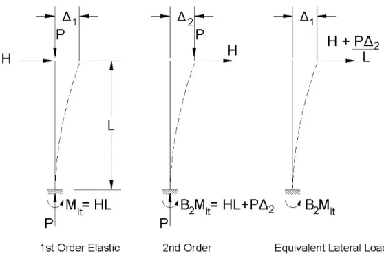
Unbraced Frames
For the case of unbraced frames, and assuming that the lateral stability for the frame in Figure 2.13 is provided by the cantilever column, the determination of the amplification factor is as follows (Geschwindner 1994):
The first order analysis moment and flexural deflections are given by
M HL (2.15) 3 1 3 HL EI (2.16)
The displacement Δ2 is the total displacement including secondary effects, and
max 2
M HL P (2.17)
An equivalent load may be determined that will result in the same moment at the bottom of the column as the second order moment.
2 P H L (2.18)
It can be seen then that the moments at the bottom of the columns for the second-order and equivalent load cases in Figure 2.13 are the same, thus the second order defection is equal to
3 2 2 3 P L H L EI (2.19) 3 3 3 2 2 2 1 3 3 3 P P L L L H EI L EI L EI 3 2 2 1 3 P L L EI Solving for Δ2 1 2 3 1 3 P L L EI (2.20)
Because the amplification factor, B2 is equal to Δ2/Δ1 and
3 1 3 HL EI , then
2 2 3 1 1 1 1 1 1 3 B P P L L H L EI 2 1 1 1 B P HL (2.22)
Because the frame is part of a complete structure, this equation can be modified to include all the loads in a story. Therefore the amplification factor for a sway column is given by the following equation (ASIC 2005):
2 1 1 u oh B P HL
(2.23)Column Strength Curves
After obtaining the internals forces, including secondary effects, of a structure from a structural analysis, the next step is to obtain the column compressive strength from the AISC equations in Chapter H of the AISC Specification. While the effective length factor takes into account global geometrical imperfections, that is, column out of plumbness, the column strength curve provides the strength of the column considering local geometrical imperfections and material imperfections. These imperfections are the out of straightness and residual stresses respectively.
Early versions of column strength date to the 1800’s when empirical formulas based on the results of column tests were used. However these formulas were limited
to the material and geometry for which the tests were performed. Another formula for the strength determination of columns which was very popular in early 1900’s, was the Perry-Robertson formula. This formula considers a column with an initial deformation and the failure of such column will occur when the maximum compression stress at the extreme fiber reaches the yield strength of the material (Ziemian 2010).
However, the studies that led to the development of the Perry-Robertson and secant formula, were based only on initial out-of-straightness and eccentrically loaded column models, along with an assumed elastic response; in addition, those expressions did not consider the presence of residual stresses. The 1961 AISC Specification presented a new formula for columns whose mode of failure was due to inelastic buckling. This new formula was based on the recommendations of the Column Research Council (CRC). The formula suggested by CRC assumes that the upper limit of elastic buckling failure is defined by an average column stress equal to one-half of yield stress. For years the column formulas found in most common specifications were strictly tangent modulus expressions combined with a safety factor (AISC 1961).
In the late 1960’s and early 1970’s, studies provided the basis for the development of a solution method based on an incremental, iterative numerical routine which established the load deflection curve for the column (Geschwindner 1994). These studies took into account residual stress, initial out-of-straightness,
spread of plasticity, and load-deflection curves were determined. The correlation of the computation results with full scale tests was good and in the order of 5 percent of the test values (Bjorhovde 1972).
The studies mentioned above, were part of a research program led by Lehigh University for the development of column curves in the U.S. Bjorhovde, in his PH.D dissertation “Deterministic and probabilistic approaches to the strength of steel columns” at Lehigh University, examined the characteristics of column strength of an extensive database for the maximum strengths of centrally loaded columns (Figure 2.14). The study encompassed a variety of different shapes, steel grades and manufacturing methods. Bjorhovde observed that there were groupings within the curves and from these, three curves were subdivided. These three column curves are known as the SSRC column strength curves 1, 2 and 3 (Bjorhovde 1972).
The commentary to the AISC Specification states that the AISC LRFD column curve represents a reasonable conversion of the research data into a single design curve and is essentially the same curve as the SSRC column curve 2P (AISC 2005). The AISC Specification column equations are actually based on the strength of an equivalent pin-ended column of length KL, with a mean maximum out-of-straigtness at is mid length of approximately KL/1500 (Ziemian 2010).
Summary of Present State of Knowledge
In addition to length, cross-section dimensions and material properties, the maximum strength of steel columns depends on the residual stress magnitude and distribution, the shape and magnitude of the initial out-of-straightness and the end restraints. The effects of these three latter variables are discussed in more detail in Chapter III.
CHAPTER III:
3COLUMN THEORY
Since the beginning of human times, columns in structures were built with large cross-sectional dimensions, thus most likely carried loads well below their potential load carrying capacity, and most likely were designed with little or no engineering in the way it is understood today (Geschwindner 1994). With the introduction of steel as a construction material and the development of higher strength steels, column stability and structural stability of steel structures has become a primary concern.
A column, or compression member, is one of the most critical structural elements of a structure, because it transfer loads from one point of the structure to another, and eventually to the foundation, through compression or a combination of compression and flexural bending. Compression members are used as compression chords in trusses as well, and as in the case of pony truss bridges, may be used as pedestrian bridges. In the case of moment or sway frames, the columns and the beams that frame into, and the connections between them, provide lateral stability to those frames. However, for the most part, discussion of column strength in common literature focuses on an individual column rather than the entire system.
This basic column, which is typically used for the derivation of stability and column strength formulas, has no imperfections and is supposed to be supported by perfect hinges; in addition, this column, also known as the perfect column or ideal
column and is referred to as a pinned column, one that rarely exists in actual structures. Nonetheless, the theoretical concepts of the ideal column are important in understanding column behavior for the study of beam-columns, compression elements and stability of frames. This ideal column is loaded by a vertical force P that is applied through the centroid of the section, the column is perfectly straight and follows Hooke’s law, that is, it is made of linearly elastic material.
Although a compression member or a structural column can be seen at as a simple structural member, the interaction between the responses and the characteristics of the material, the cross section, the method of fabrication, the imperfections and other geometric factors, and end conditions, make the column one of the most complex individual structural elements (Geschwindner 1994).
Mechanism of Buckling
Load carrying members of structures may fail in a variety of ways, including flexural bending, crushing, fracture and shear. Another type of failure is referred as to buckling. For an idealized column, this is called bifurcation buckling. Figure 3.1(a) shows an idealized column consisting of two rigid bars and a rotational spring. If a load P is applied to the end of the column, the rigid bars will rotate through small angles and a moment will develop in the spring designated as point A. This moment is called the restoring moment. If the load is relative small, the restoring moment will return the column to its initial straight position, once this load is removed. Thus, it is called stable equilibrium. If the axial force is large enough, the displacement at A will
increase and the bars will go through large angles until the column collapses. Under these conditions, the column is considered to be unstable and fails by lateral buckling (Gere 2009).
Figure 3.1Elastic Stability (Adapted from Gere 2009)
Figure 3.1(b) shows three conditions of equilibrium for the idealized column as a function of the compressive load, P versus the angle of rotation, θ. The two heavy lines, one vertical and one horizontal, represent the equilibrium conditions. Point B, where the equilibrium diagram branches, is called a bifurcation point. That is, up to that point the column or structure remains stable and will return to its original position when the load is removed, thus, it is referred as stable equilibrium. If the load is removed at the critical load, point B, the column or structure would have
suffered permanent deformation but remains stable, this is called neutral equilibrium. If the load exceeds point B, the column or structure becomes unstable and fails due to buckling, this is called unstable equilibrium.
Critical Load Theory
The fundamental requirement for any column strength theory is that it must be based on the basic principles of engineering mechanics and strength of materials, while also taking into account the stress-strain relationship of the materials and reflecting geometric imperfections of all relevant kinds (Geschwindner 1994). Two basic approaches for the determination of the column critical load can be found within the basic literature for stability analysis and determination of buckling loads. The two different basic approaches are explained below and presented in this chapter.
The first or simpler approach, also known as the Euler Load or eigenvalue approach shown in Figure 3.2, attempts to determine the maximum strength of an ideal column without geometrical or material imperfections in a direct manner without calculating the deflection (Chen 1985). This approach will provide the load at which the column will buckle, in other words the load at the bifurcation point described above, without providing a full deformation history until instability occurs.
This ideal column is assumed to be loaded concentrically and the only deflections that occur at low loads are in the direction of the applied load, that is, the axial load does not produce transverse deflection until the bifurcation or buckling load is reached. This means that up to the critical load, the column remains straight
and at the critical load there exists a bifurcation of equilibrium similar to the one described above, in which the column will reach the point of instability and buckle.
Figure 3.2Column Stability (Adapted from Chen 1985)
A second approach for the determination of the buckling load relates to a more realistic column. A real column contains imperfections such as initial out-of-straightness (Figure 3.3), in this case, deflections start from the initial deflection, Δo,
at the beginning of the application of the axial load and there is no bifurcation or sudden change of deflection as load increases. Therefore, the maximum load that an out-of-straightness column can support must be calculated using an alternate
approach. A suitable approach that considers this initial deflection, but it is complex due to its nature, is known as the load-deflection method. This method is also known as a rigorous second order analysis and will be presented in Chapter IV. Through this approach the solution is found by tracing the load-deflection behavior of the beam-column through the entire range of loading up to the maximum or peak load, which is also known as the strength of the column (Chen 1985).
Euler Buckling Load
As discussed earlier, the perfect-pinned supported column, or namely ideal column, does not exist in real structures; however, it provides a simple starting point for the stability analysis of structures that are subjected to instability buckling. For example, the column in Figure 3.4(a) will fail due to instability buckling when the column displaces as shown in Figure 3.4(b). That is, assuming the column span, L, is of sufficient length so that failure due to crushing does not take place. When the buckling load is determined for this ideal column, then the following assumptions need to be made (Chen 1985):
1. The column is perfectly straight
2. The ends of the column are simply supported
3. The compressive axial load is static and applied at the centroid of the column 4. The material follows Hook’s law and is free of initial or residual stress
Figure 3.4Pin-ended supported column
The critical load is that load for which equilibrium for a straight and slightly bent configuration is possible. For relative small deflections it can be seen that the state of equilibrium is given by the following equations (Chen 1985):
The external moment is given by
_
Z external
M Py (3.1)
and the internal moment is given by 2 _ " Z Internal x x d y M EI EI x dx (3.2)
Where E is Young’s modulus, I the moment of inertia of the cross section and EI is the flexural rigidity.
In order to maintain equilibrium
_ _ 0
Z Internal Z External
M M
The differential equation for the deflected column then becomes " 0
X
Py EI y (3.3)
Dividing the above equation by EI and re-arranging the terms we obtain the following differential equation
" 0 X P y y EI (3.4)
Next, the axial parameter is defined as
2 P P k k EI EI (3.5)
And Equation 3.4 takes the form of a linear differential equation with constant coefficients
2
" 0
y k y
sin cos
y A kx B kx (3.6)
Where A and B are constants of integration. In order to determine A and B, it is necessary to apply the boundary conditions at each end of the column
0 at 0 0 at y x y x L
The first boundary condition yields
0 A 0 B 1 B 0
The second boundary condition yields
0Asin kL B 0
Which can be satisfied in two ways, if A = 0, k and P can have any value. This is known as a trivial solution.
If sin(kL) = 0, then n kL n k L
The deformed shape is obtained by
sin 0 sin n x y A kx A L (3.7)2 P 2 k P k EI EI Then 2 2 2 n EI P L (3.8)
However, from Figure 3.4, it can be seen that the value of critical load is given by the column bending in single curvature. The critical load is then given by
2 2 cr EI P L (3.9)
From the above solution of the ideal column, one can conclude that the column strength is directly proportional to the modulus of elasticity, E, and the moment of inertia, I, of the column and inversely proportional to the square of its length. Figure 3.5, known as the Euler Curve, illustrates the buckling or Euler load as a function of the column length (Gere 2009).
Figure 3.5Euler Curve
Critical Load of Beam-Columns
The second approach for the maximum or critical load determination of a beam-column is obtained by a load-deflection, also known as the classical differential solution for beam-columns. Beam-columns are members that are subjected to axial forces and bending moments simultaneously. A typical load-deflection relation for beam-columns is shown in Figure 3.6. The following discussion will focus on a small deformation analysis (Chen 1985).
Figure 3.6Beam-Column (Adapted from Chen 1985)
Given the beam-column in Figure 3.6, with flexural stiffness EI, and loaded simultaneously with an axial load, P, and an arbitrary distributed transverse load q(x), the equations of equilibrium can be derived as follows
The transverse force is
0
V dV V q x dx Therefore, dV q x
0dx (3.10)
0 dM dy 0
M dM M Vdx Pdy V P
dx dx
(3.11)
Taking the derivative of the moment equation (Equation 3.11) and substituting in Equation 3.10,
2 2 2 2 d M Pd y q x dx dx (3.12)From small deformation analysis and assuming that the column is loaded in the elastic range and follows Hook’s law, the defection is related to the curvature by the following expression,
2 2
2 2
d y M M EI d yEI
dx EI dx
(3.13)
The differential equation has the form
4 2 4 2 d y d y EI P q x dx dx (3.14)The axial parameter is k P k2 P
EI EI therefore,
4 2 2 4 2 q x d y d y k dx dx EI (3.15)Equation 3.15 is a forth-order linear differential equation that may be solved rigorously by the use of formal mathematics (Chen 1985). Figure 3.7 shows the plot of the exact solution for a beam-column with two different initial deformations.
Unlike the perfect column, which remains straight up to the Euler load, the initially deformed column begins to bend as soon as the load is applied. It can be seen that the deflection in the beam-column increases slowly at a small ratios of the applied load to the Euler load. However, as the applied load increases, the deflection increases more rapidly and it grows exponentially with no limit at load ratios near the Euler load. Thus, the carrying capacity of an imperfect column is smaller than the Euler load, regardless of how small the initial imperfection is.
The solution of Equation 3.15 is presented in Chapter VII along with the solution of a cantilever column. These two different benchmark problems, along with their rigorous differential solutions, will be used to evaluate the computer program employed throughout this research work. The two problems mentioned above are presented in the Appendix 7 of the AISC Specifications (AISC 2005), (AISC 2010). These benchmark problems are used for the evaluation of any analysis method, including computer programs that would be used as a rigorous second-order analysis method for the determination of second-order forces required by the AISC Specifications (AISC 2005), (AISC 2010).
Figure 3.7Elastic analysis of initially deformed column (Adapted from Chen 1985)
Second Order Effects
So far the critical load of an individual column has been discussed without consideration of the interaction between the column and other members that are part of a framed structure. This interaction can significantly impact the behavior of a column that is part of a frame structure. For example, the resulting moment from a beam in a moment frame structure, which is transferred to a beam-column from a rigid or moment connection, would cause an initial deformation, and together with the compressive load acting on the column, would cause an additional moment. This additional moment is the result of the eccentricity between the applied load and the centroid of the column. The additional moment would then cause additional
deflections, these deflections would cause additional moments and so forth. Therefore, second order effects are the direct result of displacements or deformations of the structure. Common elastic methods for structural analysis assume that all deformations are small and do not account for these secondary effects.
Second order effects may be determined by a complete second order inelastic analysis (also called advanced analysis and is discussed in Chapter IV) that will take into account the actual deformations of the structure and the resulting forces in addition to the sequence of loading and spread of plasticity. This approach is more complex than necessary for normal design (Geschwindner 1994). Another method which is more common for the determination of second order effects is known as a
P-Δ analysis, which is an iterative elastic analysis to approximate the inelastic conditions. In this method a first order analysis, as described above, is carried out. The elastic deformations are determined from the resulting forces of the elastic first order analysis. Secondary moments and deformations are determined by applying the loads on the deformed structure. In order to determine the critical load of a structure, this process is repeated, incrementing the load until the analysis shows that the structure has become unstable.
A third approach used in common practice is to approximate the second order effects by amplifying the first order moments by an amplification factor. The derivation of the amplification factors was discussed previously in Chapter II
For the critical load assessment and stability analysis of a structure, it is important to understand the two different deflection components that will influence the secondary effects in the beam-column. Referring to Figure 3.8, the moment component, Pδ, shown in Figure 3.8(a) is the additional moment along the length of the member that results from the eccentricity between the centroid of the column and the deflected shape of the column. This eccentricity is caused by, either, the first-order moment, M, or by an initial geometrical imperfection (i.e. member out-of-straightnes). In this case the ends remain in the original position, in other words, there is no joint translation. This effect is known as the member effect or P-δ. The second component is shown in Figure 3.8b. For example, when the column is part of a sway frame (i.e. there is joint translation), the displaced structure will cause an additional moment, M = P(Δ). This secondary moment is the second order effect on the structure and is known as the structure effect or P-Δ. On an unbraced structure, the total second order effect on a column is given by the combined influence of the member effect (P-δ) and the structure effect (P-Δ). However, neglecting the effect of P-δ in the analysis of sway structures with large gravity loads can result in very erroneous second-order moments and forces. A discussion of neglecting P-δ and its effects is presented in Chapter VII.
One thing to keep in mind is that the member effect and the structure effect are not only caused by transverse or lateral forces, but also by member imperfections