Modeling and Prediction of Amorphous Solid Dispersion Formation Using a Molecular Descriptor

(1)

Duquesne University

Duquesne Scholarship Collection

Electronic Theses and Dissertations

Spring 5-10-2019

Modeling and Prediction of Amorphous Solid

Dispersion Formation Using a Molecular

Descriptor

Kevin DeBoyace

Follow this and additional works at:https://dsc.duq.edu/etd

Part of thePharmaceutics and Drug Design Commons

This One-year Embargo is brought to you for free and open access by Duquesne Scholarship Collection. It has been accepted for inclusion in Electronic Theses and Dissertations by an authorized administrator of Duquesne Scholarship Collection.

Recommended Citation

DeBoyace, K. (2019). Modeling and Prediction of Amorphous Solid Dispersion Formation Using a Molecular Descriptor (Doctoral dissertation, Duquesne University). Retrieved fromhttps://dsc.duq.edu/etd/1783

(2)

MODELING AND PREDICTION OF AMORPHOUS SOLID DISPERSION FORMATION USING A MOLECULAR DESCRIPTOR

A Dissertation

Submitted to the School of Pharmaceutical Sciences

Duquesne University

In partial fulfillment of the requirements for the degree of Doctor of Philosophy

By

Kevin DeBoyace

(3)

Copyright by Kevin DeBoyace

(4)

MODELING AND PREDICTION OF AMORPHOUS SOLID DISPERSION FORMATION USING A MOLECULAR DESCRIPTOR

By

Kevin DeBoyace Approved March 27th_{, 2019}

________________________________ Peter L. D. Wildfong, Ph.D.

Associate Professor of Pharmaceutics Graduate School of Pharmaceutical Sciences (Committee Chair)

________________________________ Ira Buckner, Ph.D.

Associate Professor of Pharmaceutics Graduate School of Pharmaceutical Sciences (Committee Member)

________________________________ Carl Anderson, Ph.D.

Associate Professor of Pharmaceutics Graduate School of Pharmaceutical Sciences (Committee Member)

________________________________ Kenneth Morris, Ph.D.

University Professor

College of Pharmacy and Health Services, Long Island University

(Committee Member)

________________________________ Tonglei Li, Ph.D.

Professor of Industrial and Physical Pharmacy, College of Pharmacy, Purdue University

(Committee Member)

________________________________ James K. Drennen III, Ph.D.

Associate Dean for Research and Graduate Programs

Graduate School of Pharmaceutical Sciences

________________________________ J. Douglas Bricker, Ph.D.

Dean, School of Pharmacy and Graduate School of Pharmaceutical Sciences

(5)

ABSTRACT

MODELING AND PREDICTION OF AMORPHOUS SOLID DISPERSION FORMATION USING A MOLECULAR DESCRIPTOR

By

Kevin DeBoyace May 2019

Dissertation supervised by: Peter L.D. Wildfong, Ph.D.

Poor aqueous solubility of an active pharmaceutical ingredient (API) is a significant hurdle during drug development. Delivering a drug in its amorphous solid-state is a potential method to overcome this issue, since the amorphous form has increased apparent aqueous solubility. However, the amorphous state is only metastable, and is thermodynamically driven to recrystallize. As a result, pure amorphous drugs are seldom used in marketed products. Intimately mixing a drug in its amorphous form with a polymer, known as an amorphous solid dispersion (ASD), has the potential to significantly extend the physical stability of the amorphous form, while maintaining the benefit of increased apparent solubility. However, ASDs remain poorly understood. As a result, ASDs are primarily developed using a trial and error approach, resulting in increased costs and extended time to market. A method for predicting the probability of successful formation

(6)

of intimate mixtures of drug and polymer without recrystallization (a.k.a. dispersability) has the potential to reduce costs, shorten development time, and advance scientific understanding of ASDs.

The central hypothesis of this work is that there exists a combination of materials properties that correlates with the probability that an ASD will form in PVPva. Since molecular descriptors are mathematical representations of properties of a molecule, it is hypothesized that they can be successfully applied to predict the formation of amorphous solid dispersions. Specifically, the molecular descriptor R3m was investigated as a tool for the prediction of ASD formation. The work presented herein addresses 3 primary aims: (1) investigating the statistical validity of the model by expanding the model to include 2 preparation methods and 2 concentrations, (2) advancing the understanding of the physicochemical meaning of the R3m descriptor to improve the interpretability of the descriptor, and (3) investigating the relationship between R3m and solubility.

(7)

DEDICATION

For my wife Megan

For her patience, support, patience, encouragement, and patience.

In memory of Danny

(8)

ACKNOWLEDGEMENT

Ray Bradbury said “jump off the cliff and learn how to make wings on the way down.” That’s certainly how it felt when I resigned from my industry position to pursue a PhD in Pharmaceutics at Duquesne. But it is clear that I made the right decision. I have learned more than I could have imagined, and met many wonderful people along the way. I could not have completed this work without the help and support of many of those people. I’d like to sincerely thank:

• My advisor - Dr. Peter L.D. Wildfong. Some of the best advice I heard when applying to graduate school was to pick an advisor, not a school. I’m glad that I took this advice, and I could not have asked for a better mentor.

• My co-advisor - Dr. Ira S. Buckner. An excellent teacher who has always given excellent scientific advice and helped me overcome my fear of thermodynamics.

• The members of my committee - Dr. Carl A. Anderson, Dr. Tonglei Li, Dr. Kenneth Morris, and Dr. Jeffry Madura, for their invaluable scientific input.

• The past and present members of the Wildfong and Buckner Labs: Dipy Vasa, Jeffrey Katz, Rahul Roopwani, Namita Dalal, Akshata Nevrekar, Christine Zdaniewski, David Donehue, Ashwini Gumireddy, and Mustafa Bookwala. Each of them has helped me to become a better scientist. I’d especially like to thank Dipy Vasa for being an excellent mentor and friend.

• AbbVie, Inc. - for providing funding for much of the work described in this dissertation. I’d particularly like to thank Dr. Yuchuan Gong and Dr. Deliang Zhou for their scientific input throughout the project.

(9)

LIST OF TABLES

Page

Table 1: Compilation of molecular descriptors used for prediction related to amorphous

API or ASDs. Variables which require experimental work to determine are bolded. ... 49

Table 2: Final dispersability inferences based on interpretations of data from the suite of

analytical techniques outlined in Figure 23. A value of 1 indicates successful dispersion

of the API in PVPva, while a 0 indicates failure to disperse in PVPva. R3m values listed

for each compound were calculated as outlined in the Methods section, using Equation

(16). ... 104

Table 3: Modeling statistics for R3m models of dispersability in PVPva prepared by

either the M/Q or S/E methods. The abbreviation LR refers to the likelihood ratio. ... 109

Table 4: Summary of data derived from the topology, weighted mass, and leverage

components of R3m. ... 132

Table 5: Summary of data derived from the molecular matrix (M) and influence/distance

matrix (R) components of R3m. ... 140

Table 6: Logistic regression model statistics for relevant molecular descriptors and

physicochemical properties. ... 154

Table 7: Logistic regression models for R-GETAWAY descriptors with differing atomic

mass weighting, ... 156

Table 8: Logistic regression models for R-GETAWAY descriptors which consider atom

topology = 3, but different weightings (u = unweighted, v = van der Waals volume, e =

Sanderson electronegativity, p = polarizability, + = maximal). ... 158

Table 9: Predicted and actual (where available) amorphous densities for library API.

Experimentally determined densities were obtained from the literature. ... 181

(16)

Table 11: Solubility parameter data for select library API. ... 202

Table 12: Results Summary – Melt Quench 75:25% w/w (API: PVPva). The final

inferences are made based on observations made from the suite of analytical techniques. ... 237

Table 13: Results Summary – Melt Quench 15:85% w/w (API: PVPva). The final

Table 14: Results Summary – Solvent Evaporation 75:25% w/w (API: PVPva). The final

Table 15: Results Summary – Solvent Evaporation 15:85% w/w (API:PVPva). The final

Table 16: (a) Solubility rankings were assigned based on the classifications proposed in

USP 34. (b) Solubility rankings are shown for the library compounds. ABT-348 and

Itraconazole had the lowest solubility in methanol. ... 240

Table 17: Modeling statistics for solvent evaporation R3m models. The abbreviation LR

refers to the likelihood ratio. Removing the most poorly soluble compounds (Itraconazole

and ABT-348) resulted in an increased likelihood ratio, and therefore, lower p-value.

However, removal of these compounds from the model is inadvisable due to the potential

for bias. ... 241

Table 18: Statistical assessment of solvent evaporation models with solubility rank as an

additional covariate. The drop in deviance tests indicated that adding solubility rank had

no statistically significant improvement over R3m alone. ... 241

Table 19: List of all 176 drugs used for multiple linear regression of molecular

descriptors. Library API are indicated in bold. ... 244

Table 20: List of all 80 API used to examine the relationship between R3m calculated by

CORINA generated 3D structures and 3D structures obtained from the CCDC. CCDC

refcodes are given in parentheses. ... 260

(17)

LIST OF FIGURES

Page

Figure 1: Theoretical figure illustrating both drug-polymer solubility and miscibility.

(Adapted from the Journal of Pharmaceutical Sciences, Vol 99(7), F. Qian, J. Huang, M.

A. Hussain., Drug–Polymer Solubility and Miscibility: Stability Consideration and

Practical Challenges in Amorphous Solid Dispersion Development, Pages No.

thermodynamically stable mixtures, Zones III and IV indicate meta-stable zones, and

Zones V and VI are unstable zones where recrystallization is certain within a timeframe

dictated by the molecular mobility of mixtures. ... 8

Figure 2: Envisioned formulation tool to speed development of ASDs. Future work could

also focus on applying molecular descriptors to create models for predicting long-term

physical stability of ASDs. ... 12

Figure 3: Logistic regression model showing that R3m is predictive of API (75%w/w)

dispersability in PVPva.48 _{Red triangles indicate data used to build the model, while}

yellow squares indicate 3 compounds used to test the model. ... 14

Figure 4: Categorizations of miscibility based on differences in Hildebrand solubility

parameter between components, as proposed by Hoftyzer and Van Krevelen,52

Greenhalgh et al.,70_{and Forster et al.}75_{... 25}

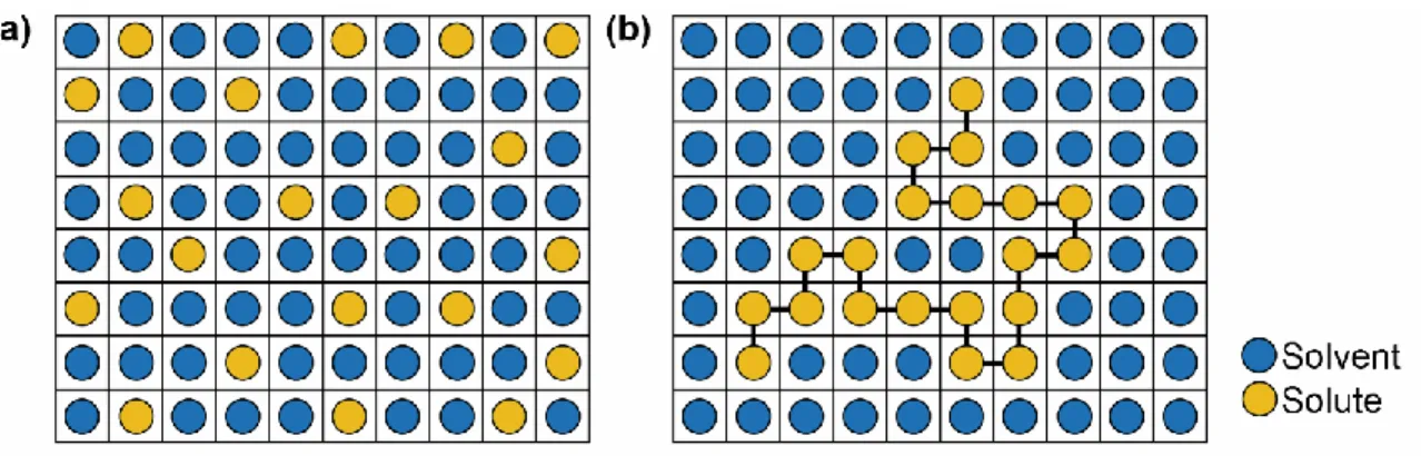
Figure 5: Visualization of the liquid lattice theory. (a) Solute and solvent molecules are

assumed virtually identical in size, spatial configuration, and external force field. (b) A

chain polymer occupies the liquid lattice, resulting in changes to configuration entropy.

(18)

Figure 6: (a) Hansen solubility based interaction parameters and their predicted

miscibility with PEG 6000, where 𝜒 < 0.98 was classified as ‘Type I’, 𝜒 = 5.19-28.27 was classified as ‘Type II’, and 𝜒 = 1.09-4.19 was classified as ‘Type III’. (b) Example free energy phase diagrams for API which are ‘Type I’ or miscible (green dot-dash line),

‘Type II’ or immiscible (red dotted line), and ‘Type III’ or partially miscible (yellow solid line) with PEG. Adapted from the Journal of Pharmaceutical Sciences, Vol 102(7), S.

Thakral, N.K. Thakral, Prediction of drug-polymer miscibility through the use of

solubility parameter based Flory-Huggins interaction parameter and the experimental

permission from Elsevier.87_{... 32}

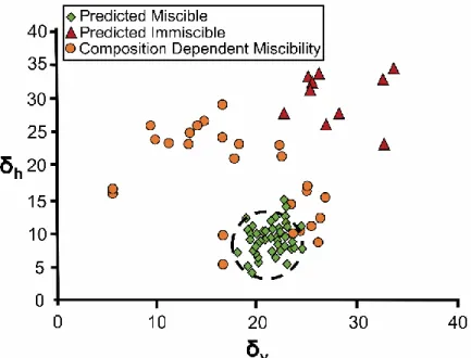
Figure 7: Bagley plot of PEG 6000 with a series of drugs. PEG 6000 is located at the

center of the black dotted circle, and compounds within the radius of the circle are

expected to be miscible with the polymer. The key refers to predictions made using the

FHIP. The Bagley plot appears to offer a better separation between predicted immiscible

and partially miscible compounds. Adapted from the Journal of Pharmaceutical Sciences,

Vol 102(7), S. Thakral, N.K. Thakral, Prediction of drug-polymer miscibility through the

use of solubility parameter based Flory-Huggins interaction parameter and the

with permission from Elsevier.87_{... 33}

Figure 8: Comparison of the (a) melting point depression30_{and (b) recrystallization}

methods93_{for approximating the equilibrium solubility, and subsequently, the interaction}

parameter (𝜒). ... 36 Figure 9: Theoretical Drug-Polymer Phase Diagram. Adapted with permission from Y.

Tian, J. Booth, E. Meehan, D.S. Jones, S. Li, G.P. Andrews, Construction of Drug–

Polymer Thermodynamic Phase Diagrams Using Flory–Huggins Interaction Theory:

(19)

Chemical Society.101_{The area above the drug-polymer solubility curve will be a stable,}

one phase system. Co-solidified mixtures at drug fractions and temperatures below the

spinodal curve are predicted to phase separate. Between the spinodal and solubility curve,

the system is expected to be metastable. ... 40

Figure 10: Visualization of the impact of the reciprocal transformation to linearity used

in equation (14) on the statistical validity of Flory-Huggins phase diagrams.106_{(a) The}

extrapolated confidence intervals are shown, indicating poor confidence in the predicted

interaction parameter at lower, pharmaceutically relevant temperatures. (b) Comparison

of the least squares estimate of equation (14) using raw data and (c) using average values.

The best fit line varies significantly, ultimately resulting in opposite inferences regarding

miscibility. Adapted from the Journal of Pharmaceutical Sciences, 105(1), M.M. Knopp,

N.E. Olesen, Y. Huang, R. Holm, T. Rades, Statistical Analysis of a Method to Predict

Elsevier.106_{... 42}

Figure 11: The QSAR/QSPR approach. Figure adapted from Gasteiger.34_{... 45}

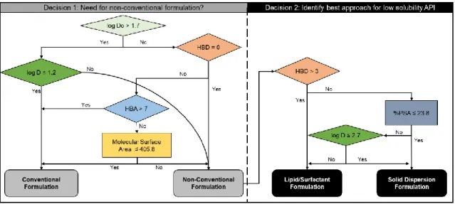
Figure 12: Example decision tree process. Adapted from the European Journal of

Pharmaceutical Sciences, S. Branchu, P.G. Rogueda, A.P. Plumb, W.G. Cook, A

decision-support tool for the formulation of orally active, poorly soluble compounds,

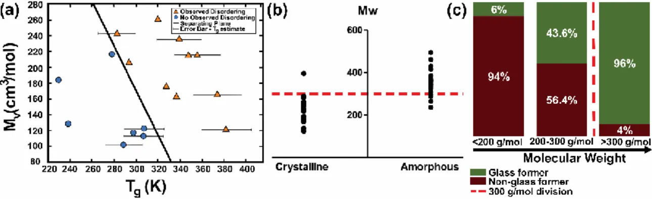
Figure 13: The relationship of GFA with Mv and MW. (a) A logistic regression model

predicting amorphization by mechanical activation. Adapted from the Journal of

Pharmaceutical Sciences, Vol 98(8), Y. Lin, R.P. Cogdill, P.L.D. Wildfong, Informatic

Calibration of a Materials Properties Database for Predictive Assessment of

Mechanically Activated Disordering Potential for Small Molecule Organic Solids, Pages

(20)

where Tg was predicted from Tm. (b) Relationship between MW and GFA. A cutoff of

300 g/mol is indicated by the red dotted line. 50 compounds are shown with 90% correctly

sorted using MW alone. Reprinted from the European Journal of Pharmaceutical

Sciences, Vol 49(2), D. Mahlin, C.A.S. Bergstrӧm, Early drug development predictions of glass-forming ability and physical stability of drugs, Pages No. 323-332, Copyright

2013, with permission from Elsevier.45_{(c) MW is a good predictor of GFA except in the}

200-300 g/mol range (based on data obtained from Alhalaweh et al.46_{). ... 53}

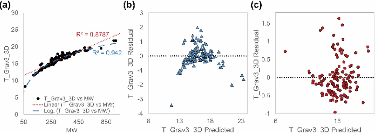
Figure 14: High correlation observed between MW and T_Grav3_3D. (a) The linear and

logarithmic relationship between MW and T_Grav3_3D indicates that the improved

prediction of GFA using T_Grav3_3D may have occurred only by chance. (b) The

residuals vs. predicted plot shows a potential violation of the assumption of linearity. (c)

Logarithmic transformation of MW appears to correct this. These figures were based on

data obtained from Alhalaweh et al.46_{... 54}

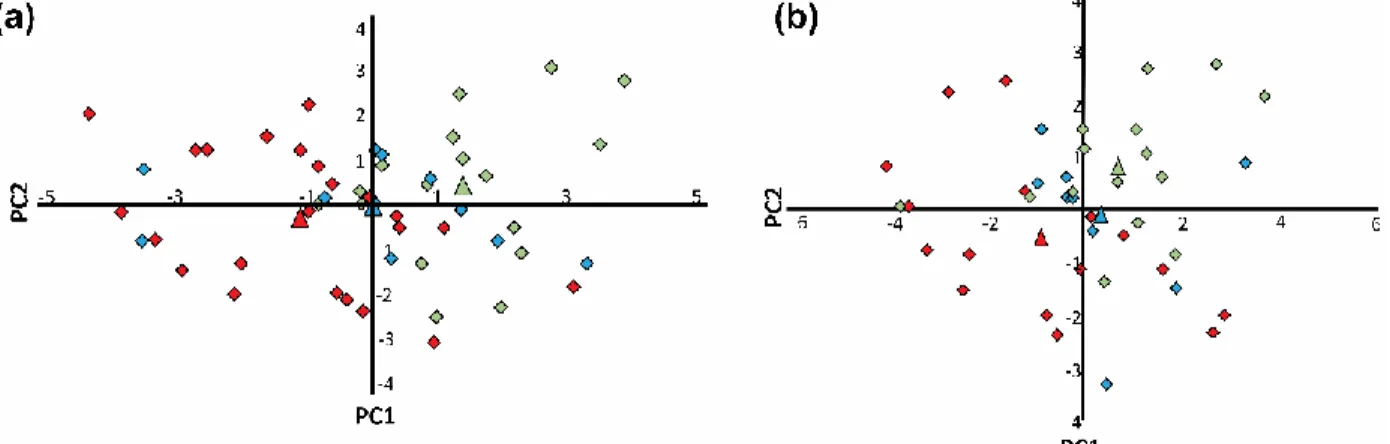
Figure 15: Principal component analysis model scores plots colored according to

crystallization tendency: (a) From undercooled melts (Adapted from the Journal of

Pharmaceutical Sciences, Vol 99(9), J.A. Baird, B. Van Eerdenbrugh, L.S. Taylor, A

Classification System to Assess the Crystallization Tendency of Organic Molecules from

Elsevier).96_{(b) From rapid solvent evaporation (Adapted from the Journal of}

Pharmaceutical Sciences, Vol 99(9), B. Van Eerdenbrugh, J.A. Baird, L.S. Taylor,

Crystallization Tendency of Active Pharmaceutical Ingredients Following Rapid Solvent

Evaporation—Classification and Comparison with Crystallization Tendency from Under

Class I (red), class II (blue), class III (green). Diamonds represent individual molecules

(21)

to generate both models, but the 3rd_{principal component is not shown since it did not}

contribute to discrimination.96_{... 57}

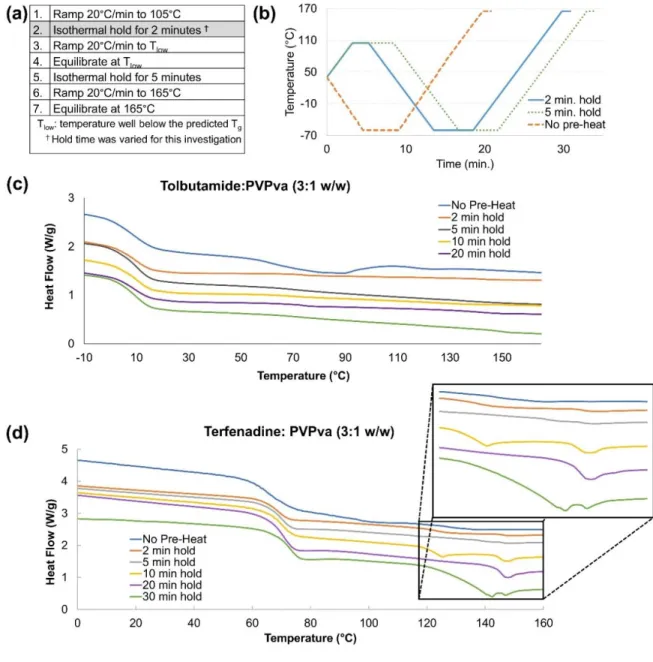
Figure 16: (a) General DSC method, (b) A plot visualizing example DSC methods where

Tlow = -60°C, c) representative DSC thermograms for tolbutamide:PVPva (3:1 w/w) and

d) terfenadine:PVPva (3:1 w/w) subject to increasing isothermal holds (105°C) prior to

initiation of temperature program. ... 77

Figure 17: Characterization of terfenadine:PVPva following 24 h of storage at room

temperature over P2O5 and with an additional 1 hour storage at 105 °C; (a) PLM image

showing small crystallites after 24 h over P2O5. (b) PLM image showing significant

crystal growth after an additional 1 h storage period in an oven at 105°C. (c) DSC

thermogram showing a significant increase in melting enthalpy after storage at 105°C for

1 h. (d) PXRD diffractograms show no detectable crystallinity in the co-solidified mixture

after 24 h over P2O5 (green diffractogram), but characteristic peaks are apparent after the

1 h storage period at 105°C (orange diffractogram) when compared to the diffractogram

of crystalline, as received terfenadine (black diffractogram). ... 80

Figure 18: Characterization of tolbutamide:PVPva following 24 h of storage at room

temperature over P2O5 and with an additional 1 h storage at 105 °C; (a) PLM image

showing no birefringence after 24 h over P2O5. (b) PLM image showing no change after

an additional 1 h storage period in an oven at 105°C. (c) DSC thermogram showing no

significant difference after storage at 105°C for 1 h. (d) PXRD diffractograms show no

detectable crystallinity in the co-solidified mixture after 24 h over P2O5 (yellow

diffractogram), or after the 1 h storage period at 105°C (blue diffractogram) as compared

to the crystalline, as received tolbutamide (black diffractogram). As received tolbutamide

was determined to be polymorph I (see Figure 55a in the Appendix, CSD-ZZZPUS02)155,

(22)

Figure 19: HSM of terfenadine:PVPva (3:1 w/w) stored at room temperature over P2O5

for 24 h. A heating ramp of 10°C/min was applied. (a) 25°C (b) 105°C (c) Isotherm at

105°C for 15 min (d) Isothermal at 105°C for 30 min (e) Isothermal at 105°C for 60 min.

Crystallization of terfenadine is observed. ... 85

Figure 20: 9 month aged Tolbutamide:PVPva (3:1 w/w) DSC analysis ... 86

Figure 21: HSM of tolbutamide:PVPva (3:1 w/w) aged at room temperature over P2O5

for 9 months. A heating ramp of 10 °C/min was applied. (a) 25 °C (b) 80 °C (c) 90 °C (d)

100 °C (e) isothermal at 105 °C for 1 min. Re-dissolution of the tolbutamide into the

polymer is observed. ... 87

Figure 22: Molecular structures of API in the compound library. ... 94

Figure 23: Representative characterization data for several compounds in the library. (a)

PXRD data confirm crystallinity in quinidine 15% (S/E) co-solidified mixtures. Note:

Quinidine recrystallized as a methanolate (CSD ID: MUHZUM18). Cimetidine 15%

(M/Q) is X-ray amorphous, as indicated by the absence of diffraction peaks. (b) DSC data

representing three potential outcomes: Ketoconazole 15% (M/Q) appears to be dispersed,

based on the appearance of a single Tg. Melatonin 15% (M/Q) is phase separated, as

indicated by the presence of 2 distinct Tg’s. Quinidine 15% (S/E) is partially crystalline, as indicated by the appearance of an endotherm. (c) PLM data representing two possible

outcomes: Chlorpropamide 15% (M/Q) appears amorphous, as indicated by the lack of

birefringence. Quinidine 15% (S/E) is birefringent, indicating crystallinity. (d) PDF data

representing two possible outcomes: The melatonin 75% (M/Q) co-solidified mixture

does not significantly deviate from the linear combination of the individual components,

suggesting phase separation. The felodipine 15% (S/E) co-solidified mixture does

(deviations shown in green), suggesting molecular dispersion.166_{... 100}

Figure 24: Dispersion classification decision tree. A suite of analytical techniques is

(23)

limitations of any individual technique.10 The applied analytical techniques include

powder X-ray diffraction (PXRD), differential scanning calorimetry (DSC), polarized

light microscopy (PLM), hot-stage microscopy (HSM), and analysis of pair distribution

function (PDF) transformed X-ray data... 101

Figure 25: Modeling of dichotomous classifications of API dispersability in PVPva for

co-solidified mixtures prepared by (a) melt quenching and (b) solvent evaporation,

against the molecular descriptor R3m. Separation is observed in the melt quench models;

all API having R3m > 0.65 were dispersable in PVPva. Logistic regression was used to

model solvent evaporation behavior. Increasing values of R3m are still well correlated

with dispersability in PVPva. ... 108

Figure 26: The logistic regression model for dispersability predictions of 15% w/w API

in PVPva improved when itraconazole and ABT-348 are excluded (indicated with x

symbols), relative to the original model at this drug loading. ... 113

Figure 27: Scatter plot showing the relationship between R3m and both molecular weight

(circles) and average molecular weight (triangles). The solid blue and dotted orange lines

show the linear regression of both molecular weight and average molecular weight

against R3m, respectively. ... 117

Figure 28: Histograms and outlier boxplots (shown above the histograms) for the

distribution of (a) glass transition temperatures and (b) melting temperatures for model

compounds (in Kelvin). The blue box indicates the interquartile range. The red line within

the box indicates the median. Whiskers indicate the largest and smallest value in the

distribution, excluding outliers. The red cross marks indicate outliers from a normal

distribution. ABT-102, ABT-072, and ABT-348 all have higher glass transition and

melting temperatures than the other library compounds. The boxplot indicates that in

(24)

co-solidified mixtures prepared by (a) melt-quenching and (b) solvent evaporation,

against the molecular descriptor R3m. Separation is observed in the melt-quench models;

all API having R3m >0.65 were dispersible in PVPva. Logistic regression was used to

model solvent evaporation behavior. Increasing values of R3m are still well correlated

with dispersability in PVPva. Reproduced from Chapter 4, Figure 25 for convenience. ... 126

Figure 30: Illustrations of the impact of some matrices relevant to the calculation of R3m.

Indomethacin is used here as an example. (a) A topological distance is illustrated with

the N6 nitrogen in indomethacin. Arrows indicate 7 topological connections to nitrogen

equal to 3 (excludes hydrogens for clarity). When hydrogens are included, the number of

connections for N6 increases to 11. (b) The distance from the geometric center of the

molecule is indicated with a red-white-blue color scheme, (c) the leverage values for each

of the atoms in indomethacin are given (excludes some hydrogens for clarity). ... 131

Figure 31: The impact of iterative changes to the number of carbons in a (a) linear chain

and (b) cyclic systems. ... 135

Figure 32: An illustration of the effect of 3D conformation on leverage used to calculate

R3m. (a) Atom labels for library compound chlorpropamide. Example conformations 1

and 2 of chlorpropamide are shown in (b) and (c), respectively, with corresponding R3m

values shown beneath. (d) A bar plot of the leverages which result from the respective

conformations. Hydrogen atoms are excluded from the bar plot for clarity. ... 142

Figure 33: Felodipine. (a) 2D structure with atom numbers labeled. Visual representation

(matrices and bar plots) of data relevant to the calculation of R3m: (b) molecular matrix,

(c) topology matrix, (d) geometry matrix, (e) influence/distance matrix, (f) bar plot of

weighted mass, (g) contribution to R3m, (h) bar plot of leverages. ... 152

Figure 34: Bar plots showing the correlation coefficient (r) between R3m and other

(25)

topological distances within the library (green bars). (b) The correlation between R3m

and other descriptors with different weightings (u = unweighted, v = van der Waals

volume, e = Sanderson electronegativity, p = polarizability, + = maximal) within the API

library (orange bars). ... 155

Figure 35: The relationship between R3m and average molecular weight (AMW) for a

dataset of 176 API. ... 160

Figure 36: A multiple linear regression model of molecular weight and molecular density

vs. R3m. (a) a 3D surface plot showing the linear fit as a surface (R2_{= 0.59), (b) the actual}

vs. predicted plot. ... 161

Figure 37: Correlation coefficient (r) between molecular weight and other descriptors

which describe API shape, volume and area. ... 162

Figure 38: Molecular structures of API in the M/Q compound library with R3m values

given parenthetically. ... 167

co-solidified mixtures prepared by melt-quenching against the molecular descriptor R3m.

Separation is observed in the melt quench models, where all API having R3m > 0.65 were

dispersable in PVPva.48, 174_{Reproduced here from Figure 25a, for convenience. ... 168}

Figure 40: Example molecular dynamics simulation. (a) The conformer tool is used to

identify the lowest energy conformation (black dashed line). (b) This conformation is

used to construct 10 amorphous cells. The 3 with the lowest energy (indicated in orange)

are selected for MD simulations. (c) The MD simulation using the NPT ensemble.

Multiple frames are selected after equilibration (indicated by the red boxes). (d) The

selected frames are saved and coordinates are extracted using MATLAB to calculate R3m

values for each individual molecule. (e) Some example conformations from a single MD

(26)

Figure 41: Histograms of the average absolute difference between R3m values calculated

using CORINA and R3m calculated using crystal structures obtained from the CCDC.

(a) 80 API, and (b) 130 API, which included 50 polymorphic forms of the original 80

compounds. Linear relationship between (c) R3m values for 80 API calculated using 3D

structures from CCDC vs. the CORINA algorithm, and (d) R3m values for 80 API (blue

diamonds) and 50 polymorphic forms for a total of 130 API (orange circles). The orange

regression line reflects the fit for all 130 API. Points indicated by the red box show R3m

values calculated for the different polymorphs of aripiprazole. ... 177

Figure 42: (a) Molecular structure of aripiprazole. (b) A comparison of the CCDC

structures obtained for 2 aripiprazole polymorphs, where the dichlorophenyl groups are

overlaid on the left. The change in 3D coordinates results in a relatively significant

difference in R3m values (aripiprazole I (CCDC ID: MELFIT01,184_{orange) R3m = 0.951,}

aripiprazole VII (CCDC ID: MELFIT07,185_{teal) R3m =1.204). ... 178}

Figure 43: A box-and-whisker plot of the R3m values calculated from MD simulations

(840 R3m values for each API). The red line toward the center of the box is the median,

the box shows the interquartile range, and the whiskers indicate the interquartile range

multiplied by 1.5. Values outside of this range have the red ‘+’ symbol, indicating values that fall outside of a normal distribution. The black diamonds indicate the mean, and the

blue dashed lines indicate the R3m values calculated from SMILES files and the

CORINA algorithm. The horizontal black dotted line indicates the original R3m decision

boundary, and the horizontal black dot-dashed line indicates the boundary updated using

MD simulation results (R3m=0.632, see Figure 45). The green boxes indicate API which

were experimentally observed to successfully form ASDs using the melt quench method,

while those API in red indicate compounds which failed to form ASDs. ... 182

Figure 44: Propranolol conformations and their effect on R3m. (a) Propranolol with

(27)

conformation ((b) and (c)). (b) The propranolol molecule in red was extracted from MD

simulations and has an R3m value equal to the median. (c) The green propranolol

molecule shows a conformation from the MD simulation having an R3m value most

similar to the CORINA conformation (difference in R3m = 0.0014). ... 184

Figure 45: Logistic regression model using the expanded MD dataset. This model

contains 12,600 data points for R3m (jittered to more clearly show the amount of data).

Red circles correspond to API which failed to form an ASD in PVPva by melt-quenching,

while green circles correspond to API which were observed to successfully form an ASD

in PVPva by melt-quenching. The blue line shows the logistic curve. This expanded

model resulted in an updated boundary value of 0.632. The equation for the regression

line and the standard errors of the coefficients are given. ... 186

Figure 46: Theoretical figure illustrating both drug-polymer solubility and miscibility.

(Adapted from the Journal of Pharmaceutical Sciences, Vol 99(7), F. Qian, J. Huang, M.

A. Hussain., Drug–Polymer Solubility and Miscibility: Stability Consideration and

Practical Challenges in Amorphous Solid Dispersion Development, Pages No.

thermodynamically stable mixtures, Zones III and IV indicate meta-stable zones, and

Zones V and VI are unstable zones where recrystallization is certain within a timeframe

dictated by the molecular mobility of mixtures. Of particular interest to this chapter is the

red solid line representing crystalline API-polymer solubility. Reproduced from Figure 1

for convenience. ... 191

Figure 47: Experimental setup for dissolution end-point experiments. Cryomilling was

performed for multiple durations and an optimal duration was identified using both

PXRD and DSC. PXRD was used to qualitatively confirm that crystals remain. DSC was

(28)

changes in Tend (ΔTend ≲0.5 °C). The optimal milling duration was then replicated to

obtain n = 5-9 measurements of Tend. ... 199

Figure 48: The relationship between the Hansen Partial Solubility Parameters and R3m.

(a) The dispersion Hansen partial solubility parameter, (b) the polar Hansen partial

solubility parameter, (c) the hydrogen-bond Hansen partial solubility parameter, and (d)

the 3-D solubility parameter, where the Euclidean distance between PVPva and the

selected drugs is determined (0 is PVPva). ... 203

Figure 49: Example data collected during optimization of cryomilling duration.

Ketoconazole: PVPva 50:50% w/w. (a) PXRD data, (b) DSC data, (c) a bar plot of

replicate Tend measurements at different milling durations. No significant changes in the

experimentally determined dissolution end point are observed after 16 minutes of

cryomilling. ... 206

Figure 50: Example data collected during optimization of cryomilling duration.

Indomethacin: PVPva 50:50% w/w. (a) PXRD data, (b) DSC data, (c) a bar plot of

replicate Tend measurements at different milling durations. The optimal milling duration

was identified as 12 minutes in this case. After 12 minutes, the endotherm became more

difficult to analyze, and at 24 minutes of milling the endotherm was essentially absent,

and therefore Tend could not be determined. ... 207

Figure 51: Experimental data for the determination of API solubility in PVPva at different

temperature using the Van’t Hoff equation. API plotted as triangles are those API which

failed to disperse in PVPva by melt-quenching, while circles indicate API that

successfully formed ASDs by melt-quenching. ... 209

Figure 52: Experimental data for the determination of API solubility in PVPva at different

temperatures. The dotted lines show the Van’t Hoff extrapolation to lower temperature. Triangles are used for API which had previously been show to fail to form an ASD in

(29)

ASD in PVPva. Plots of the predicted Tg for each API determined using the

Couchman-Karasz equation are shown as solid and dot-dash lines. ... 210

Figure 53: Weight percent solubility at the predicted glass transition temperature for 15%

(circles) and 75% (squares) drug loading vs. R3m. The horizontal blue and red lines are

included to reference the drug loading of interest (15 and 75% API). The vertical dashed

line shows the previously established R3m boundary (R3m = 0.65). ... 211

Figure 54: Evidence of Terfenadine polymorphs. DSC method adapted from Leitǎo et

al.154_{... 235}

Figure 55: Tolbutamide polymorphs. (a) Tolbutamide was received as the Form I

polymorph, as evident when comparing the experimental PXRD pattern with the

reference pattern (CSD-ZZZPUS02).155, 156_{(b) After several months of storage,}

Tolbutamide appears to recrystallize as the Form II polymorph, as shown by comparison

of the experimental PXRD pattern to the reference pattern (CSD-ZZZPUS15).156, 208_{... 236}

Figure 56: Multiple logistic regression model of 15% w/w API in PVPva with R3m and

solubility ranking as covariates. (a) A 3-D plot showing the logistic regression surface

that results from inclusion of solubility ranking as a covariate. (b) Comparison of

univariate (R3m only) and multivariate (R3m and solubility ranking) model statistics.

AUC (ROC) = area under the receiver operating characteristic curve. ... 242

Figure 57: Multiple logistic regression model of 75% w/w API in PVPva with R3m and

solubility ranking as covariates. (a) A 3-D plot showing the logistic regression surface

that results from inclusion of solubility ranking as a covariate. (b) Comparison of

univariate (R3m only) and multivariate (R3m and solubility ranking) model statistics.

AUC (ROC) = area under the receiver operating characteristic curve. ... 242

co-solidified mixtures prepared by (a) melt quenching and (b) solvent evaporation,

(30)

all API having R3m > 0.65 were dispersable in PVPva. Logistic regression was used to

model solvent evaporation behavior. Labels have been added to compounds having:

variations between preparation methods, outcomes which vary with concentration, and/or

relatively low solubility in methanol. See section 4 (discussion) for additional details. ... 243

Figure 59: Bicalutamide. (a) 2D structure with atom numbers labeled. Visual

representation (matrices and bar plots) of data relevant to the calculation of R3m: (b)

molecular matrix, (c) topology matrix, (d) geometry matrix, (e) influence/distance matrix,

(f) bar plot of weighted mass, (g) contribution to R3m, (h) bar plot of leverages... 245

Figure 60: Chlorpropamide. (a) 2D structure with atom numbers labeled. Visual

Figure 61: Cimetidine. (a) 2D structure with atom numbers labeled. Visual representation

Figure 62: Cloperastine. (a) 2D structure with atom numbers labeled. Visual

Figure 63: Felodipine. (a) 2D structure with atom numbers labeled. Visual representation

Figure 64: Indomethacin. (a) 2D structure with atom numbers labeled. Visual

(31)

Figure 65: Itraconazole. (a) 2D structure with atom numbers labeled. Visual

Figure 66: Ketoconazole. (a) 2D structure with atom numbers labeled. Visual

Figure 67: Melatonin. (a) 2D structure with atom numbers labeled. Visual representation

Figure 68: Nifedipine. (a) 2D structure with atom numbers labeled. Visual representation

Figure 69: Propranolol. (a) 2D structure with atom numbers labeled. Visual

Figure 70: Quinidine. (a) 2D structure with atom numbers labeled. Visual representation

(32)

Figure 71: Sulfanilamide. (a) 2D structure with atom numbers labeled. Visual

Figure 72: Terfenadine. (a) 2D structure with atom numbers labeled. Visual

Figure 73: Tolbutamide. (a) 2D structure with atom numbers labeled. Visual

Figure 74: The impact of the size of the amorphous cell on the results of molecular

dynamics calculations. (a) An amorphous cell containing 40 ketoconazole molecules, (b)

an amorphous cell containing 200 ketoconazole molecules, (c) the resulting distributions

of R3m after a molecular dynamics simulation. The blue bars are for the 200 molecule

simulation, resulting in 1400 R3m values, while the orange bars are for the simulations

containing 40 molecules (3 replicates for a total of 840 R3m values). ... 261

Figure 75: A comparison of R3m values calculated from 3-D conformations generated

from the CORINA algorithm, obtained from crystal structure data, and generated by

molecular dynamic simulations. R3m values calculated using CORINA and CCDC

structures fall within the range of values determined using molecular dynamics. ... 262

Figure 76: A plot of predicted % solubility vs. Temperature. The solid lines correspond

to the van’t Hoff extrapolation. The dotted lines correspond to the Couchman-Karasz predicted Tg values. The gray dotted lines illustrate the determination of the solubility at

(33)

the concentration of the prepared dispersion was used to identify the relevant % solubility.

(34)

LIST OF ABBREVIATIONS

3D Three-dimensional

AMW Average molecular weight API Active pharmaceutical ingredient ASD Amorphous solid dispersion

BCS Biopharmaceutics classification system Cp Heat capacity (constant pressure) CCDC Cambridge crystallographic data center DFT Density functional theory

DSC Differential scanning calorimetry FF Force field

FHIP Flory-Huggins interaction parameter

G Geometry Matrix

GC Group contribution

GETAWAY Geometry topology and atom weight assembly GFA Glass forming ability

H Molecular influence matrix ∆Hmix Enthalpy of mixing

HME Hot melt extrusion HSM Hot stage microscopy

M Molecular matrix

(35)

MLR Multiple linear regression

Mv Molar volume

M/Q Melt quench MW Molecular weight

PCA Principal component analysis PDF Pair distribution function PEG Polyethylene glycol

PLM Polarized light microscopy PLS Partial least squares

PVP Polyvinylpyrrolidone

PVPva Polyvinylpyrrolidone vinyl acetate, also known as copovidone PXRD Powder X-ray diffraction

QSPR Quantitative structure-property relationship R Influence/distance matrix

R3m R-GETAWAY third order autocorrelation index weighted by atomic mass RTm R-GETAWAY total index weighted by atomic mass

∆Smix Entropy of mixing S/E Solvent evaporation SP Solubility parameters SVM Support vector machines

Tend Dissolution end point temperature Tg Glass transition temperature Tm Melting temperature

(36)

Chapter 1.

Introduction

1.1.

Statement of Problem

Overcoming limitations associated with the poor aqueous solubility of an active pharmaceutical ingredient (API) is a significant hurdle during drug development. Poor aqueous solubility will result in drug dissolution limitations and, therefore, limitations to bioavailability. Delivering a drug in its amorphous solid-state is a potential method to ameliorate this issue, since the amorphous form increases the apparent aqueous solubility of the drug. However, amorphous solids are metastable and thermodynamically driven to recrystallize. As a result, pure amorphous drugs are seldom used in marketed products. Intimately mixing a drug in its amorphous form with a polymer, known as an amorphous solid dispersion (ASD), has the potential to significantly extend the physical stability of the amorphous form, while maintaining the benefit of increased apparent solubility.

ASDs represent an important formulation strategy for addressing poor aqueous solubility of API. It is estimated that approximately 40% of highly potent compounds fail to reach clinical trials owing to their inability to dissolve well in aqueous media,1 and approximately 50% of new drug candidates require formulation help to improve solubility and delivery.2 ASDs have the potential to increase the apparent solubility of a drug, while also increasing the physical stability relative to the pure component amorphous drug substance.

Although ASDs were introduced to pharmaceutical drug delivery more than 50 years ago,3_{their formation and physical stability remains poorly understood,}4_{with only a few} specific exceptions. Proposed stabilizing mechanisms include API crystallization

(37)

inhibition5_{and anti-plasticization effects that reduce molecular mobility,}6_while dispersions are generally thought to form as the result of specific non-covalent bonding interactions between drug and polymer carrier, such as hydrogen-bonds.7, 8 Presently, reliable prediction of ASD formation and persistence is not possible, and, therefore, requires experimental confirmation. As a result, ASD formulation development must often be performed using trial-and-error, which can result in significantly increased development costs and delays to market. The challenges imposed by this formulation strategy are evident from the relatively few commercially available ASDs.9_{Models that can assist with rational} selection of excipients for ASD formulations are desirable for improvement of formulation development, reduction of costs, and reduced time to market.

1.2.

Literature Review

1.2.1.

Methods for Improving Aqueous Solubility

A large portion of newly developed drug candidates have poor aqueous solubility, and several formulation strategies (both chemical and physical) have been developed in an attempt to increase solubility. These include the use of salt forms, particle size reduction, higher energy polymorphs,10_{co-crystallization,}11_{and amorphous solid molecular} dispersions. However, there is no universally applicable method for increasing solubility, and each of these strategies has potential pitfalls.

Formulation of salt forms is not always practical, and if they are synthesized, they may undergo reconversion to their acid or base forms, resulting in no significant benefit in dissolution rate.12_{Additionally, potassium and sodium salts may react with atmospheric}

(38)

carbon dioxide and water to precipitate out as their original parent compounds, especially in the outer layer of a dosage form, resulting in reduced rates of dissolution.13 Particle size reduction will increase API solubility due to the increased surface area of the drug crystals. However, improvement in apparent solubility via reducing particle size has practical limitations, not the least of which is the minimum size to which a particle can be reduced relative to the energy input from comminution equipment.14_{Also, small particles can have} a negative impact on downstream unit operations (owing to their poor flow, poor wettability, etc.). Additionally, mechanical force may induce solid state phase transformations such as polymorphism (e.g., as seen in chlorpropamide15) or amorphization,16 which may result in poor control over the final solid form of the API, and subsequent undesirable batch-to-batch variability in dissolution rate and/or bioavailability.

High energy polymorphs of the API of interest will also yield solubility benefits due to a reduction in the number of non-bonded interactions. However, the application of metastable polymorphs is limited to those that are sufficiently kinetically stable over a pharmaceutically relevant timescale.

Co-crystallization has the potential to yield increases in solubility while maintaining thermodynamic stability and potentially avoiding issues associated with polymorphic transformations. But, co-crystallization can also lead to deteriorated pharmaceutical properties in some cases (e.g., further decrease in solubility) and may exhibit its own polymorphism.11

Formulations that use the amorphous form of a drug have many challenges, but there has been increased interest in this approach owing to the approval of several formulations

(39)

by the FDA.17_{In addition, solid dispersions may be beneficial over some other techniques} due to lower manufacturing costs and smaller pill burden.4

1.2.2.

Amorphous Solid Dispersions

1.2.2.1. Brief History

Amorphous solid dispersions are intimate mixtures of polymer and API that increase apparent aqueous solubility via inhibition of crystallization. The historical background of solid dispersions is laid out well in the review article by Chiou and Riegelman.13 Briefly, a unique technique for preparation of dispersions of small particles in an inert matrix was demonstrated by Sekiguchi and Obi in 1961. They prepared eutectic mixtures by melting and rapidly cooling binary mixtures.3 This resulted in a significant increase in drug delivery from this mixture as compared to the crystalline form of the API alone. This premise was later extended to the preparation of glasses due to the even greater increase in solubility offered by the amorphous form.18

1.2.2.2. Manufacturing Methods

Methods for preparation of amorphous solid dispersions include melting, solvent evaporation, and the melting-solvent method.13 The melting-solvent method involves dissolving the API in a suitable solvent followed by mixing with a molten polymer. This method is less popular in the literature due to limitations in drug loading and concerns about the inclusion of solvent in the final formulation. This approach will, therefore, not be discussed further in this document.

(40)

The melting method is performed by co-melting the polymer and API at a temperature above the API melting temperature and above the polymer glass transition temperature and/or melting temperature (if applicable). After melting, the liquid mixture is rapidly cooled so that the API is kinetically unable to nucleate and grow in its crystal form. In contrast, the solvent method requires dissolution of the API and polymer in a common solvent followed by rapid evaporation of that solvent. As with the melt quench method, rapid evaporation and subsequent solidification reduces the likelihood of nucleation and subsequent growth of crystals.

It is important to note that while both the solvent and melting methods may be used to formulate an amorphous dispersion, there is evidence to suggest that the resulting formulations are not completely molecularly similar. It has been proposed that thermal history is an important determinant of the physical properties of the resulting amorphous dispersion.19_{Differences in experienced stresses are thought to result in different enthalpic} states. Additionally, it is reasonable to expect dissimilarity between preparation methods due to the introduction of a ternary component in solvent evaporation. A change in the number of molecular interactions occurring as a result of the presence of a solvent could result in differences in the final state of the dispersion.

It has been shown that preparation method can have a significant impact on the resulting solid.20-23 In addition to these concerns, certain small molecules may be more amenable to certain manufacturing methods. For example, if the compound is thermally labile, a solvent evaporation method would be more suitable. Conversely, if the compound is not sufficiently soluble in preferred organic solvents, a melt method may be preferable.

(41)

1.2.2.3. Miscibility, Solubility, and Dispersability

Dispersability is defined herein as the successful formation of an ASD by intimate mixing of API and polymer followed by co-solidification without crystallization. Miscibility is defined as a mixture of drug and polymer “consisting of a single chemically

homogeneous phase where all of the components are intimately mixed at the molecular

level, and the properties of the blend are different from the properties of the pure

components.” 9_{The important distinction between dispersability and miscibility is a} consequence of: (1) the analytical limitations inherent to the detection of phase separation and (2) the thermodynamics of the system (miscibility) versus the kinetics (dispersability).

The current analytical limitations make it difficult to definitively identify the presence of a homogeneous system. For example, differential scanning calorimetry (DSC) is commonly used to assess miscibility, but Utracki et al. point out that “a single Tg is not a measure of miscibility, but only of the state of dispersion.”24_{Phase separation may still} occur over time. Additionally, it may not be possible to detect phase separation for domains <30 nm, or when the glass transitions of the pure components are within 10°C of each other.25 Even heating the sample during DSC can result in changes to miscibility that may be misinterpreted as representing the initial physical state of the sample (see Chapter 3).

Another example of an analytical limitation can be seen in powder x-ray diffraction (PXRD). This method can be used to detect the lack of an ordered crystalline phase, but will not be able to determine if a system is phase separated without more advanced data analysis. One such advanced method is pair distribution function (PDF) analysis, which can be applied to assess changes in the fingerprint of interatomic distances for co-solidified mixtures compared to the amorphous pure components.26_{However, this method will be}

(42)

more sensitive as higher energy x-rays are employed, such as a synchrotron source, which is not routinely available to research labs. Copper anodes, which are most popular for laboratory x-ray diffractometers, may not always generate PDF data that contain enough information to be definitive.27 The application of a suite of analytical techniques will increase the certainty of conclusions.28 However, there is currently no analytical method which can definitively detect phase separation in every case.

The distinction between solubility and miscibility has been reviewed by Qian et al,4

and is illustrated in Figure 1 which is adapted from the same. The solid red line represents the crystalline API solubility in the polymer, whereas the dashed blue line indicates the amorphous API-polymer miscibility.

(43)

Figure 1: Theoretical figure illustrating both drug-polymer solubility and miscibility. (Adapted from the Journal of Pharmaceutical Sciences, Vol 99(7), F. Qian, J. Huang, M. A. Hussain., Drug–Polymer Solubility and Miscibility: Stability Consideration and Practical Challenges in Amorphous Solid Dispersion Development, Pages No. 2941-2947, Copyright 2010, with permission from Elsevier).4 Zones I and II indicate thermodynamically stable mixtures, Zones III and IV indicate meta-stable zones, and Zones V and VI are unstable zones where recrystallization is certain within a timeframe dictated by the molecular mobility of mixtures.

Solubility is defined as the analytical composition of a saturated solution, where the solid and solubilized form of a molecule are in equilibrium.29 Solubility is perhaps most commonly applied in pharmaceutical science to assess the amount of drug that will dissolve in a particular volume of a solvent such as water. It is also possible for a polymer to dissolve a drug to some extent when in the liquid state. The API is often considered the ‘solvent’ in this case, merely because of its smaller size. This API-polymer solubility is indicated by the red solid line in Figure 1. This line indicates a boundary between a thermodynamically stable state and a thermodynamically metastable state.

(44)

The equilibrium associated with miscibility is given by Equation (1), and the IUPAC definition for miscibility is given in Equation (2).29 Miscibility describes the successful formation of a homogenous phase through liquid-liquid mixing;30 specifically in this document the liquid-liquid mixing of polymer and amorphous API.

(1) APIamorphous+ Polymeramorphous ⇌ API/Polymeramorphous,homogenous phase

(2) (∂2ΔGmix

∂ϕ2

)

T,p

> 0

The blue dashed line boundary corresponding to the amorphous API-polymer miscibility is a boundary between a thermodynamically metastable state and an unstable state, where eventual recrystallization is certain.4 This boundary also represents conditions where Equation (2) is equal to zero.

The application of miscibility in this context comes from polymer physics, where the individual components are generally stable in the amorphous state. The application of the concept to systems in which the thermodynamically stable state is crystalline (i.e., API), results in added complexity.4 A thermodynamically stable state will be achieved in Zones I and II shown in the figure, a meta-stable state occurs in Zones III and IV, and an unstable or crystallized co-solidified mixture in Zones V and VI. It is important to note that this figure is theoretical, and measurements of solubility and miscibility at temperatures below the Tg cannot be obtained experimentally, and, therefore, can only be estimated through extrapolation.4 Methods for such extrapolations will be discussed in more detail in Chapter 7.

As stated above, dispersability is defined here as the successful formation of an amorphous solid dispersion by intimate mixing with a carrier polymer, followed by co-solidification without recrystallization. Both miscibility and solubility lack a clear physical

(45)

meaning below the glass transition temperature of the system because increasing viscosity prohibits the system from reaching equilibrium.4 Also noted above, the extrapolation of miscibility to lower temperatures is only theoretical. Dispersability differs from these equilibrium states because it is expected to also encapsulate kinetic factors. While miscibility and solubility refer to equilibrium states, dispersability may also capture important factors that occur during formation of the solid binary mixtures. For example, a system that is expected to phase separate and/or crystallize based on inferences about the equilibrium state could remain dispersed due to rapid solidification.

1.2.2.4. Predicting dispersability

Currently there is no proven, rapid, and cost-effective way to assess the dispersability of API in polymers. As a result, determinations of dispersability have been primarily performed by trial-and-error.

Some current research has been focused on streamlining component screening for amorphous solid dispersions. Shanbhag et al. developed an automated screening method using 96-well plates to screen an API against 6 polymers and 8 surfactants to identify leads for solid dispersion formulations.31 However, screening was performed using the solvent method while melt extrusion was the unit operation of interest for manufacturing at large scale. As noted previously, potential differences in molecular interaction between these methods would suggest that the solvent method may be inappropriate for predicting performance of the melt method. Verma and Rudraraju developed a systematic four-phase approach to formulation design of amorphous solid dispersions.32 They detail a stepwise method for assessment of API, screening against polymers, prediction of miscibility, and

(46)

confirmation of predictions. While their method is thorough and useful for development of amorphous solid dispersions, it is time consuming and requires a significant amount of drug for testing. Typically during early pre-formulation studies gram quantities of API are often scarce, presenting a limitation to industrial application of this work.

Predictions related to what is defined herein as dispersability have been relatively infrequent in the literature. Existing research tends to be more focused on the development of models to assess and predict miscibility or solubility in amorphous solid dispersions, with the goal of predicting the physical stabili