Improving the Performance of MO-RV-GOMEA on Problems
with Many Objectives using Tchebycheff Scalarizations
Ngoc Hoang Luong
Centrum Wiskunde & Informatica Amsterdam, The Netherlands
Tanja Alderliesten
Academic Medical Center Amsterdam, The Netherlands
Peter A. N. Bosman
Centrum Wiskunde & Informatica Amsterdam, The Netherlands
ABSTRACT
The Multi-Objective Real-Valued Gene-pool Optimal Mixing Evo-lutionary Algorithm (MO-RV-GOMEA) has been shown to exhibit excellent performance in solving various bi-objective benchmark and real-world problems. We assess the competence of MO-RV-GOMEA in tackling many-objective problems, which are normally defined as problems with at least four conflicting objectives. Most Pareto dominance-based Multi-Objective Evolutionary Algorithms (MOEAs) typically diminish in performance if the number of ob-jectives is more than three because selection pressure toward the Pareto-optimal front is lost. This is potentially less of an issue for MO-RV-GOMEA because its variation operator creates each off-spring solution by iteratively altering a currently existing solution in a few decision variables each time, and changes are only ac-cepted if they result in a Pareto improvement. For most MOEAs, integrating scalarization methods is potentially beneficial in the many-objective context. Here, we investigate the possibility of im-proving the performance of MO-RV-GOMEA by further guiding improvement checks during solution variation in MO-RV-GOMEA with carefully constructed Tchebycheff scalarizations. Results ob-tained from experiments performed on a selection of well-known problems from the DTLZ and WFG test suites show that MO-RV-GOMEA is by design already well-suited for many-objective prob-lems. Moreover, by enhancing it with Tchebycheff scalarizations, it outperforms MOEA/D-2TCHMFI, a state-of-the-art decomposition-based MOEA.
CCS CONCEPTS
·Mathematics of computing→Evolutionary algorithms;
KEYWORDS
Multi-objective optimization, Tchebyche scalarization
ACM Reference Format:
Ngoc Hoang Luong, Tanja Alderliesten, and Peter A. N. Bosman. 2018. Improving the Performance of MO-RV-GOMEA on Problems with Many Objectives using Tchebycheff Scalarizations. InGECCO ’18: Genetic and
Evolutionary Computation Conference, July 15–19, 2018, Kyoto, Japan.ACM,
New York, NY, USA, 8 pages. https://doi.org/10.1145/3205455.3205498
Permission to make digital or hard copies of all or part of this work for personal or classroom use is granted without fee provided that copies are not made or distributed for profit or commercial advantage and that copies bear this notice and the full citation on the first page. Copyrights for components of this work owned by others than ACM must be honored. Abstracting with credit is permitted. To copy otherwise, or republish, to post on servers or to redistribute to lists, requires prior specific permission and/or a fee. Request permissions from [email protected].
GECCO ’18, July 15–19, 2018, Kyoto, Japan
© 2018 Association for Computing Machinery. ACM ISBN 978-1-4503-5618-3/18/07. . . $15.00 https://doi.org/10.1145/3205455.3205498
1
INTRODUCTION
The Multi-Objective Real-Valued Gene-pool Optimal Mixing Evolu-tionary Algorithm (MO-RV-GOMEA), a recently-introduced mem-ber of the GOMEA family, is a state-of-the-art Multi-Objective Evolutionary Algorithm (MOEA) for the continuous domain that exhibits both superior scalability on benchmark problems [6] and excellent performance on real-world applications [16]. MO-RV-GOMEA is characterized by three main features. First, explicit link-age models that align with dependencies among decision variables of the problem instance under consideration are either constructed during optimization by performing linkage learning on the working population (in black-box optimization), or are defineda prioriby using available problem-specific knowledge (in gray/white-box op-timization). Second, a variation operator, named Gene-pool Optimal Mixing (GOM), is used to exploit the learned linkage information during solution variation in an effective manner such that offspring solutions are guaranteed to have equal or better fitness values than parent solutions. Third, a niching concept is realized in MO-RV-GOMEA by a cluster-based operation, i.e., in every generation, solutions in the population are partitioned into equal-sized clusters; linkage learning and solution variation can then be performed per cluster, thereby increasing the probability that all different regions of the Pareto-optimal front are evenly approached.
A key feature of GOMEAs is that the GOM variation operator of GOMEAs transforms an existing solution into an offspring solution through a series of so-calledmixingevents. Each mixing event is a partial solution alteration that involves only decision variables that are dependent on each other to some degree (as indicated by the learned, ora prioridefined, linkage models). Each partially-altered solution is then evaluated for improvement and the new decision variable values are only accepted if the fitness value of the solution does not deteriorate. This native genetic-local-search-like variation operator makes partial evaluations straightforward to be imple-mented in GOMEAs if the problem permits efficient computation of the effect of changing values of a few decision variables. For many other Evolutionary Algorithms (EAs), such partial evalua-tions are non-trivial or impractical to be implemented because a whole offspring solution is created each time without intermediate improvement checks as in GOM. Partial evaluations substantially increase the performance of MO-RV-GOMEA, especially in real-world applications where each full solution evaluation typically incurs a considerable amount of computation cost (e.g., see [16]).
However, while succeeding in solving complicated problems with thousands of decision variables, MO-RV-GOMEA has mainly been tested on bi-objective optimization problems [6, 16]. The per-formance of MO-RV-GOMEA on problems that have more than two
objectives is yet to be investigated. Especially the class of many-objective problems, which is often defined as problems that have at least four objectives, poses substantial challenges for many MOEAs. The primary difficulty is that as the number of objectives increases, using the Pareto dominance relation in selection based on an entire population does not effectively maintain (selection) pressure toward the Pareto-optimal front since most solutions in the population of an MOEA are non-dominated [1, 12].
In recent years, the class of decomposition-based MOEAs has emerged as a more effective methodology for tackling multi- and es-pecially many-objective problems. A decomposition-based MOEA typically decomposes a multi-objective problem into a set of single-objective optimization subproblems, in which each subproblem is a scalarization of the original problem, i.e., aggregating all objectives on the basis of a unique weight vector. A diverse set of weight vectors is normally used to create a well-spread set of scalarization functions, aiming to evenly approximate the Pareto-optimal front. Selection pressure is maintained by using scalar improvements associated with the scalarization functions (which are similar to single-objective optimization) rather than depending on Pareto dominance improvements. The well-known MOEA based on De-composition (MOEA/D) [19] presents three options for performing aggregation: the weighted-sum approach, the weighted Tcheby-cheff method, and the Penalty-based Boundary Intersection (PBI) method. The latter two are more commonly used since they are able to obtain solutions on non-convex regions, if such exist, of Pareto-optimal fronts. The Tchebycheff method is more convenient to use since it does not require the user to define the penalty factor
θas in the PBI method, which can have significant influence on the performance of the search [12]. Many MOEA/D variants have been proposed to provide improvements on several aspects of the original MOEA/D [22]. The recently-introduced Nondominated Sorting Genetic Algorithm III (NSGA-III) [9] also employs weight vectors in the form of reference points to improve the performance of the well-known NSGA-II when solving many-objective problems. Therefore, in this paper, besides benchmarking MO-RV-GOMEA in the many-objective realm, we also investigate the possibility of employing the Tchebycheff method to enhance the performance of the original MO-RV-GOMEA.
The remainder of the paper is organized as follows. In Section 2, we outline MO-RV-GOMEA. In Section 3, we propose our approach to integrate the Tchebycheff aggregation function into MO-RV-GOMEA. Optimization problems employed for benchmarking and our experiment settings are described in Section 4. Results are discussed in Section 5. Finally, conclusions are drawn in Section 6.
2
MO-RV-GOMEA OUTLINE
MO-RV-GOMEA maintains a populationPofNcandidate solutions (i.e., population members), which can be randomly initialized, as well as an elitist archive to keep track of non-dominated solutions obtained during the search because elitism is beneficial to conver-gence [13]. Until the termination criteria are satisfied, the following procedure is performed in every generation. First, non-dominated ranks of all solutions are determined and truncation selection is performed to select a setSthat consists of⌊τ N⌋best ranked solu-tions fromP(τ=0.35 in [6]). Second, the selected solutions inSare
then partitioned intokclusters, and anothermclusters are taken from the population (mis the number of objectives). Third, for each cluster, linkage learning is performed to construct a linkage model
F consisting of a set of linkage sets on the basis of the solutions in that cluster. A Gaussian distribution is estimated for each linkage set in the linkage model. Next, the set of estimated Gaussian distri-butions associated with each cluster is used to iteratively construct offspring solutions in a step-wise manner.
2.1
Clustering
In every generation,q=k+mclusters of candidate solutions are formed. First,kleader solutions that are far apart from each other are selected fromSby a nearest-neighbor heuristic as follows.
Step 1: The solution that has the maximum value for a randomly chosen objective is assigned as the first leader. The Euclidean dis-tances in objective space from all the remaining solutions to the first leader are computed and stored as their nearest-neighbor distances.
Step 2: The solution with the largest nearest-neighbor distance is assigned as the next leader.
Step 3: The Euclidean distance from each remaining solution to the newly assigned leader is computed and the nearest-neighbor distance is updated if the new distance is smaller than the currently stored value. Go back toStep 2untilkleaders are obtained.
Thesekleaders are then assigned as the centroids of thek clus-ters. From its centroid, each cluster is formed by expanding to cover itscnearest solutions. Thesekclusters, named middle clusters, will then be used for multi-objective dominance-based optimization. For the remainingmclusters, each of them is associated with a unique objectiveiand is formed by selecting from the population
Pthe bestcsolutions according to the corresponding objectivei. Thesemclusters, named extreme clusters, will then be used for single-objective scalar optimization along the associated objectives. All theseqclusters are called selection clusters (where each cluster
Chascmembers) as they are formed by selection procedures, and it was recommended to havec=q2|S|[6].
2.2
Linkage Learning
LetL = {1,2, . . . ,l}be the set that contains the indices of alll
decision variables. For each cluster, a linkage modelF that de-scribes the dependencies amongldecision variables is constructed. The Family-Of-Subset (FOS) concept is used as the general linkage model. Each FOS is a set of linkage setsF = {F1,F2, . . . ,F| F |}, in which linkage setFi ⊆Lcontains the indices of the decision variables that are dependent on each other to some degree. The two most common FOS structures in GOMEA literature are: 1) the univariate model, in which all variables are considered totally in-dependent; and 2) the linkage tree model, a hierarchical ordering of linkage sets in which decision variables can be considered in-dependent according to some linkage sets and can be considered dependent according to some other linkage sets. The linkage tree model can thus express hierarchical dependencies between problem variables. The goal is to configure the linkage modelF such that it aligns with the variable-dependence problem structure of the problem instance under concern. If problem-specific knowledge is available,F can be constructeda priori. Otherwise,F can be learned by linkage learning algorithms (see [6] for details).
For each linkage setFiin the (learned) linkage modelF of each selection clusterC, the parameters of a Gaussian distribution, that involves the variables encoded inFi, are estimated over the cluster solutions. Thus, a univariate Gaussian distribution (i.e., mean and variance) is estimated for a univariate linkage set, and a multivari-ate Gaussian distribution (i.e., mean vector and covariance matrix) is estimated for a multivariate linkage set. In order to alleviate the potential premature diminishing of variance due to selection, the variance parameters of these Gaussian distributions are propor-tionally scaled with the distance of improvements found from the Gaussian means. These Gaussian distributions are then used to sample new values during solution variation (more details in [6]).
2.3
Gene-pool Optimal Mixing (GOM)
Each solutionxin the population is associated with the nearest selection cluster (based on the distance betweenxand the cluster means in the objective space). This association effectively partitions the population intoqclusters, where each population clusterCP
corresponds to a selection clusterC. A variation operator named GOM is employed to transform each solutionx ∈ CP into an offspringousing the linkage modelF of clusterC.
Instead of generating a whole offspring in one step as in many MOEAs, GOM constructsoin a step-wise manner as follows. All linkage sets inF of each clusterCare iteratively considered in a random order. For each linkage setFi, its associated Gaussian distribution is used to sample new values, altering all solutions of
CP at the variables indicated byFi. These variables of a number of solutions, specifically⌊12τ|CP|⌋, are then further moved in the direction that the cluster mean is shifted in from the previous gener-ation to the current genergener-ation [6]. The partially-altered solutions are evaluated for improvement. IfCis a middle cluster, each im-provement check is based on Pareto dominance. That is, the change is accepted when the altered solution dominates the previous state or it can be accepted into the elitist archive. IfC is an extreme cluster, the change is accepted when the altered solution improves the previous state with respect to the objective associated with that extreme cluster. If no improvement is yielded, the change is revoked and the solution returns to its previous state. An offspring solution
ois fully constructed after all linkage sets inF are considered. The elitist archiveAof MO-RV-GOMEA is bounded by a user-defined target size. An adaptive mechanism maintains the archive around the target size by discretizing the objective space into equal-sized hypercubes and only retaining one archive member per hy-percube [17]. A solutionpis accepted into the archive if it is not dominated by the archive (A⪯̸p), i.e.,pis not dominated by any archive member and the hypercube thatpresides in is unoccupied orp dominates the current resident member of that hypercube. After every generation, the hypercube sizes are adapted based on the range of the so-far-obtained Pareto front and the target size.
3
MO-RV-GOMEA ADAPTATIONS
3.1
Tchebycheff Scalarization Method
The weighted Tchebycheff distance (TCH) between a pointzand a given pointz∗in anm-dimensional space is defined as follows:
TCH(z,z∗,w)= max
1≤i≤m{wi|zi−z
∗
i|} (1)
wherew = (w1, . . . ,wm) is a weight vector withwi ≥ 0 and
Pm
i=1wi =1.
A multi-objective problem withldecision variables andm ob-jective functions can be described as follows:
min x∈Ωx
f(x)=(f1(x), . . . ,fm(x)) (2) wherexis a decision variable vector in the decision space (that we assume to be real-valued in this paper),Ωx⊆Rl,f =(f1, . . . ,fm): Ωx → Ωf is them-dimensional objective function vector, and
f(x)is thus the objective value vector ofxin the objective space Ωf ⊆Rmof the multi-objective problem.
Using the weighted Tchebycheff distance with a utopian point as the pointz∗(z∗i ≤min{fi(x)|x∈Ωx}), a multi-objective problem
can be decomposed into a set of scalar optimization subproblems. Each subproblem has a unique weight vectorwand is defined as:
min x∈Ωx {TCH(f(x),z∗,w)}= min x∈Ωx { max 1≤i≤m{wi|fi(x)−z ∗ i|}} (3)
It is known that with Tchebycheff scalarizations it is possible to identify solutions on potential non-convex regions of the Pareto-optimal front [19] while this is not possible using linearly weighted sum scalarizations [7]. Therefore, Tchebycheff scalarizations are often employed in decomposition-based MOEAs.
3.2
Weight Vector Generation
Weight vectors are often generated such that they are spread as well as possible. Perfectly scatteringNpoints in ad-dimensional space (d >1), however, is NP-hard [5]. Here, we employ a simple, yet
effective, method to approximately generateNwell-spread weight vectors as follows. During initialization, we uniformly randomly generateMweight vectors such thatM>>N, where each weight vectorw satisfieswi ≥ 0 andPm
i=1wi = 1. We then apply the
same heuristic that is used to selectkleaders in thek-leader-means clustering [4] (see Section 2) to selectNvectors that are spread as well as possible. An advantage of this approach is that any number of weight vectorsNcan be generated rather than being restricted to some required numbers as in other methods (e.g., [8, 14]).
3.3
Weight Vector Association
We employ the following procedure to associate each weight vector
wwith a candidate solutionxin the current populationP.
Step 1: Compute the ideal objective vectorzP =(zP1, . . . ,zPm)
of the current populationPon the basis of the solutions inP:
ziP =min{fi(x)|x∈P} (4)
Step 2: For each weight vectorw, compute the weighted Tcheby-cheff distance withwbetween each solution in the current popula-tionPand the ideal objective vectorzP.
Step 3: Associate each weight vectorwwith the nearest solution that has not been associated yet with any weight vector, based on the Tchebycheff distances that are computed withwin Step 2.
Figure 1a shows an example that illustrates the weight vector association procedure. In every generation, our procedure above explicitly assigns anew to each solution a unique improvement re-gion (e.g., see Figure 1b). If a solution is not improved by GOM, and still remains in the next generation, it might be assigned a different improvement region. For many algorithms in the MOEA/D family,
0 0.1 0.2 0.3 0.4 0.5 0.6 0.7 0.8 0 0.1 0.2 0.3 0.4 0.5 0.6 0.7 0.8 zP=(0.2,0.2) z* w(1)=(0,1) w(2)=(1/3,2/3) w(3)=(2/3,1/3) w(4)=(1,0) y(4)=(0.7,0.2) y(3)=(0.55,0.3) y(2)=(0.3,0.45) y(1)=(0.2,0.65) TCH(y(4),zP,w(1))=0 TCH(y(4),zP,w(2))=0.17 TCH(y(4),zP,w(3))=0.33 TCH(y(4),zP,w(4))=0.5 TCH(y(3),zP,w(1))=0.1 TCH(y(3),zP,w(2))=0.12 TCH(y(3),zP,w(3))=0.23 TCH(y(3),zP,w(4))=0.35 TCH(y(2),zP,w(1))=0.25 TCH(y(2),zP,w(2))=0.17 TCH(y(2),zP,w(3))=0.08 TCH(y(2),zP,w(4))=0.1 TCH(y(1),zP,w(1))=0.45 TCH(y(1),zP,w(2))=0.3 TCH(y(1),zP,w(3))=0.15 TCH(y(1),zP,w(4))=0 Pareto Front 0 0.1 0.2 0.3 0.4 0.5 0.6 0.7 0.8 0 0.1 0.2 0.3 0.4 0.5 0.6 0.7 0.8 w(1)=(0,1) y(4)=(0.7,0.2) w(2)=(1/3,2/3) y(3)=(0.55,0.3) w(3)=(2/3,1/3) y(2)=(0.3,0.45) w(4)=(1,0) y(1)=(0.2,0.65) z* Pareto Front
a) Tchebycheff scalarizations b) Improvement regions
Figure 1: x-y axes: objectives (f1,f2). a) Weighted
Tcheby-cheff distances between 4 pointsy(i)’s and the ideal objective pointzP with 4 weight vectorsw(i)’s,i=1, . . . ,4. Bold-faced
distances indicate the association between a vectorwand a
pointy. b) Improvement region of each solution defined by
the associated weight vectorw(i)and the utopian pointz∗.
each solution is regarded as the best solution obtained so far for each subproblem. Therefore, if a solution is not changed in this generation (i.e., no offspring succeeds to replace the parent), its improvement region is still the same in the next generation. We note that there exist other weight vector association procedures in several weight vector-based MOEAs (e.g., NSGA-III [9], I-DBEA [1]). However, the association procedures in these MOEAs are mainly used for niching or diversity preservation purposes. Our associa-tion procedure here determines the improvement region for each solution and thus puts more emphasis on the exploitation purpose.
3.4
Improvement Check in GOM
Similar to the original MO-RV-GOMEA, each existing solutionxis improved by the GOM variation operator with the learned linkage model of the cluster to whichxbelongs. At every mixing event, the partially-altered solution is evaluated and checked for improvement. In the original MO-RV-GOMEA, the improvement check is based on the Pareto dominance improvement for the solutions in the middle clusters, and is based on the scalar improvement for the solutions in the extreme-region clusters. The latter is thus already a form of Tchebycheff scalarization where the weight vectorwhas weight
wi =1 for objectiveiand weight 0 for the other objectives.
We propose two options to adapt the improvement check at each mixing event in GOM with Tchebycheff scalarizations as follows:
•Option 1: The change is accepted if the partially-altered so-lutionpdominates the previous stateb, orpcan be accepted into the elitist archive, or the objective value vector ofphas a smaller Tchebycheff distance (computed with the associated weight vectorw) to the utopian pointz∗(compared to that of the previous state), i.e.,p⪯b∨A⪯̸p∨TCH(f(p),z∗,w)<
TCH(f(b),z∗,w).
•Option 2: The change is accepted ifpdominatesbor the
new objective value vector has a smaller Tchebycheff dis-tance to the utopian point, i.e.,p⪯b∨TCH(f(p),z∗,w)<
TCH(f(b),z∗,w).
Note that the utopian pointz∗employed for the improvement check is different from the population’s ideal objective vectorzP
employed for the weight vector association in Section 3.3. We here assume that the utopian pointz∗is known for the sake of conve-nience. In the case that the utopian point cannot be determineda
priori,z∗can be approximated during optimization by updatingz∗i
to the best so-far-obtained value of objectivei, if necessary, before computing the Tchebycheff distances in each improvement check.
4
BENCHMARK AND EXPERIMENT SETTING
4.1
Benchmark Problems
We perform experiments on two well-known sets of benchmark problems: DTLZ1-DTLZ4 [10] and WFG1-WFG4 [11]. For all prob-lems, the number of decision variables is scaled asl=40,80,160,
and 320. For DTLZ problems, we employ problem instances of
m = 3,5,10,and 15 objectives. For WFG problems, we employ
problem instances ofm=2,3,5,and 10 objectives, where the num-ber of position parameters and the numnum-ber of distance parameters are determined as in [2]. The reference Pareto-optimal fronts for both DTLZ and WFG problem instances are created by using the PlatEMO platform [21] such that a reference front with approxi-matelym×1000 well-distributed points is generated for a problem instance withmobjectives.
4.2
Experiment Setting
We benchmark the original MO-RV-GOMEA and its two new adap-tations with Tchebycheff scalarizations. For the purpose of compar-isons, we also experiment with the recently-introduced MOEA/D-2TCHMFI [18], an MOEA/D variant that employs the Tchebycheff scalarization withl2-norm constraint, which is defined as
TCH(f(x),z∗,w)}= max 1≤i≤m (|fi(x)−z∗ i| wi ) (5) wherewis a weight vector withwi ≥0 and∥w∥=1.
The population size is a crucial control parameter for EAs, and it is also notoriously difficult to determine an appropriate popu-lation size for an EA solving a specific problem instance. While EA benchmark literature often uses the same population size for all algorithms, we argue that such a simple setting might not be proper because different EAs have different minimally-required population sizes, and the differences can be substantial (e.g., see [20]). Therefore, in this work, we employ the so-called Interleaved Multi-start Scheme (IMS) [6] (which originates from the population-sizing-free scheme of the Parameter-less Genetic Algorithm [15]) to adapt the population size during optimization for all MOEAs. The IMS operates multiple instances of an MOEA with different population sizes in an interleaved fashion. The initial population
P0is started with a small population sizeN0.N0can be any reason-ably small population size. Here, we simply setN0=10×(m+1). A larger populationPi with sizeNi = 2×Ni−1 is started later,
and each generation ofPi is then operated for everyдgenerations of the previous populationPi−1. A smaller population is deemed
inefficient, and is thus terminated, if it contributes less than 10% of the combined front of non-dominated solutions obtained from all the working populations. All the populations are kept growing and running until the computation budget is spent. In this paper,
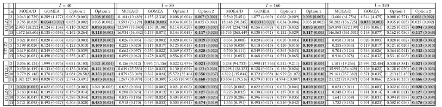
Table 1: Medians and interdecile ranges (in brackets) of the IGD metric of the approximation fronts obtained by MOEAs on solving DTLZ problems. MOEA/D, GOMEA, Option 1, and Option 2 should be read as MOEA/D-2TCHMFI, the original MO-RV-GOMEA, MO-RV-GOMEA with adaptation Option 1, and MO-RV-GOMEA with adaptation Option 2, respectively.
l=40 l=80 l=160 l=320
m MOEA/D GOMEA Option 1 Option 2 MOEA/D GOMEA Option 1 Option 2 MOEA/D GOMEA Option 1 Option 2 MOEA/D GOMEA Option 1 Option 2
D TLZ1 3 0.043 (0.729) 0.289 (1.177) 0.008 (0.003) 0.008 (0.002) 0.104 (10.489) 1.155 (2.338) 0.008 (0.004) 0.007 (0.002) 0.560 (5.451) 1.877 (4.069) 0.008 (0.009) 0.008 (0.003) 13.606 (61.756) 4.544 (4.475) 0.008 (0.571) 0.008 (0.002) 5 0.785 (8.820)0.034(0.002) 0.035 (0.002) 0.035 (0.002) 3.593 (23.129)0.034(0.003) 0.034 (0.003) 0.035 (0.002) 18.648 (50.245) 0.033(0.002) 0.034 (0.004) 0.035 (0.002) 58.282 (136.725) 0.033(0.003) 0.035 (0.005) 0.035 (0.002) 10 2.903 (18.252) 0.124 (0.134) 0.110 (0.023) 0.093(0.006) 13.599 (76.040) 0.150 (0.108) 0.114 (0.020) 0.093(0.007) 68.991 (234.734) 0.156 (0.093) 0.117 (0.032) 0.093(0.007) 169.898 (472.199) 0.170 (0.061) 0.125 (0.033) 0.094(0.005) 15 4.672 (65.606) 0.135 (0.058) 0.162 (0.264) 0.118(0.003) 16.934 (56.442) 0.133 (0.071) 0.144 (0.045) 0.117(0.028) 65.740 (365.449) 0.130 (0.071) 0.152 (0.029) 0.117(0.005) 146.863 (561.031) 0.168 (0.077) 0.162 (0.030) 0.117(0.040) D TLZ2 3 0.021 (0.003) 0.020 (0.003) 0.020 (0.003) 0.019(0.002) 0.026 (0.005) 0.020 (0.003) 0.020 (0.003) 0.019(0.002) 0.034 (0.008) 0.020 (0.003) 0.020 (0.003) 0.019(0.003) 0.050 (0.016) 0.020 (0.003) 0.020 (0.002) 0.018(0.003) 5 0.199 (0.020) 0.124 (0.014) 0.122 (0.013) 0.109(0.010) 0.225 (0.020) 0.117 (0.017) 0.125 (0.018) 0.111(0.008) 0.240 (0.030) 0.118 (0.015) 0.120 (0.015) 0.109(0.009) 0.255 (0.034) 0.119 (0.017) 0.121 (0.020) 0.113(0.013) 10 0.619 (0.084) 0.349 (0.025) 0.376 (0.039) 0.323(0.024) 0.662 (0.097) 0.350 (0.022) 0.369 (0.037) 0.328(0.022) 0.700 (0.111) 0.349 (0.031) 0.363 (0.043) 0.328(0.018) 0.704 (0.124) 0.346 (0.026) 0.364 (0.041) 0.332(0.022) 15 0.862 (0.081) 0.490 (0.020) 0.555 (0.071) 0.440(0.010) 0.899 (0.062) 0.478 (0.025) 0.556 (0.079) 0.433(0.010) 0.911 (0.053) 0.468 (0.034) 0.531 (0.065) 0.434(0.010) 0.916 (0.078) 0.467 (0.032) 0.531 (0.065) 0.435(0.010) D TLZ3 3 0.056 (0.124) 1.999 (3.976) 0.021 (0.103) 0.021 (0.004) 0.156 (0.512) 7.996 (11.156) 0.022 (2.979) 0.021(0.003) 0.238 (94.733) 11.990 (17.766) 0.512 (9.211) 0.021(0.004) 1.101 (19.266) 25.994 (32.484) 0.530 (8.881) 0.021(0.003) 5 0.450 (6.439) 0.133 (0.024) 0.132 (0.036) 0.121(0.021) 0.639 (25.583) 0.126 (0.023) 0.130 (0.029) 0.123 (0.020) 22.298 (128.323) 0.128 (0.022) 0.136 (0.026) 0.121(0.019) 35.995 (254.629) 0.129 (0.022) 0.128 (0.030) 0.119(0.023) 10 0.779 (9.148) 0.378 (0.025) 24.084 (28.582)0.353(0.043) 4.879 (53.049) 0.367 (0.024) 25.572 (32.464)0.356(0.037) 4.822 (135.844) 0.372 (0.058) 16.959 (21.072)0.351(0.040) 29.161 (257.382) 0.371 (0.035) 11.213 (25.452)0.346(0.028) 15 1.021 (27.100) 0.820 (0.952) 2.574 (3.491) 0.473(0.016) 1.267 (38.979) 0.615 (0.389) 5.145 (10.903)0.468(0.021) 10.864 (119.516) 0.579 (0.101) 4.974 (10.807)0.471(0.028) 21.122 (219.707) 0.561 (0.066) 2.516 (6.335) 0.466(0.034) D TLZ4 3 0.020 (0.003) 0.022 (0.003) 0.022 (0.003) 0.021 (0.002) 0.022 (0.004) 0.022 (0.003) 0.021 (0.002) 0.020(0.003) 0.023 (0.008) 0.022 (0.004) 0.022 (0.004) 0.020(0.002) 0.024 (0.011) 0.022 (0.003) 0.022 (0.004) 0.020(0.002) 5 0.183 (0.044) 0.139 (0.014) 0.139 (0.014) 0.130(0.017) 0.208 (0.023) 0.138 (0.013) 0.138 (0.018) 0.127(0.012) 0.223 (0.032) 0.138 (0.024) 0.137 (0.014) 0.126(0.011) 0.248 (0.051) 0.141 (0.014) 0.140 (0.021) 0.127(0.009) 10 0.564 (0.047) 0.392 (0.024) 0.386 (0.044) 0.374(0.036) 0.835 (0.186) 0.395 (0.024) 0.404 (0.037) 0.369(0.025) 1.220 (0.286) 0.396 (0.027) 0.389 (0.035) 0.372(0.037) 1.641 (0.359) 0.393 (0.031) 0.394 (0.037) 0.373(0.039) 15 0.721 (0.098) 0.495 (0.027) 0.506 (0.028) 0.485(0.024) 0.918 (0.170) 0.494 (0.033) 0.505 (0.041) 0.474(0.019) 1.353 (0.191) 0.493 (0.027) 0.510 (0.042) 0.473(0.028) 1.722 (0.185) 0.501 (0.023) 0.502 (0.056) 0.476(0.024)
we employ the generation baseд=8 as recommended in [6] for
real-valued operators and problem variables.
The published implementation of MOEA/D-2TCHMFI [18] em-ploys a specific population size with a specific set of weight vectors for each problem instance. In order to freely scale its population size in the IMS, we replace the provided fixed weight vector sets with the weight vectors generated by the procedure described in Section 3.2. The neighborhood size parameter is set as 10% of the population size. While the IMS might not be the optimal setting for an MOEA, any MOEA that is integrated with the IMS can be consid-ered as an anytime algorithm, i.e., the longer the MOEA is allowed to run, the better the results will be, and the users can terminate the algorithm whenever they are satisfied with the results.
For all problem instances, each MOEA is run 30 times indepen-dently on a multi-core server (4×AMD Opteron Processor 6386 SE, 2.8 GHz). Note that MO-RV-GOMEAs perform certain tasks (e.g., population clustering, linkage learning), which incur additional computation cost, that MOEA/D-2TCHMFI does not have. For fair comparisons, we thus employ the running time as the computa-tion budget rather than the number of funccomputa-tion evaluacomputa-tions. This effectively allows MOEA/D-2TCHMFI to perform more function evaluations than MO-RV-GOMEA. For each problem instance of
mobjectives andldecision variables, every MOEA is run form×l
seconds each time. All MOEAs are equipped with an elitist archive, and the target archive size is set empirically as 1000.
To assess the convergence of each algorithm to the reference Pareto-optimal fronts, we use the Average Front Distance (AFD) [3] that measures the average minimal Euclidean distance over all points in a reference front to an approximation front obtained by an MOEA run. The AFD is also commonly known as the Inverted Generational Distance (IGD) in the literature (e.g., [9, 18]). The median IGD value over the 30 runs of each MOEA is then used as the performance metric. To verify the statistical significance of the obtained results, we use the Mann-Whitney-Wilcoxon statistical hypothesis test for equality of medians withp<0.05. In Tables 1, 2,
and 3, the best median value for each problem instance is presented with the gray background, and is further highlighted in bold if the value is statistically significantly better than those obtained by other MOEAs (significance tests are performed with Bonferroni correction).
5
EXPERIMENTAL RESULTS
5.1
DTLZ Problems
Table 1 shows the medians and the interdecile ranges of the IGD metric of the approximation fronts obtained by MOEAs for the DTLZ1-4 problem instances. In almost all cases, MO-RV-GOMEA outperforms MOEA/D-2TCHMFI, obtaining better approximation fronts. The results in Table 1 confirm that the original design of MO-RV-GOMEA, which yields excellent, and often superior, per-formance in solving multi-objective problems [6], is also suitable for tackling many-objective problems. This suitability is likely due to the synergy between the multi-objective dominance-based opti-mization of middle clusters, the single-objective scalar optiopti-mization (along each objective) of extreme clusters, and the direct offspring versus parent comparison for accepting improvements in the oper-ation of MO-RV-GOMEA.
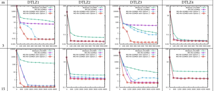
The two adaptation options with Tchebycheff scalarization that we propose in this paper assign to each population member a unique improvement region, which could be informative in guiding the search, potentially enhancing the efficiency of MO-RV-GOMEA. Ta-ble 1 shows that, for DTLZ proTa-blem instances, the performance of the original MO-RV-GOMEA has similar performance (in some cases), or deteriorates (in some cases), or is slightly improved (in other cases) when combined with Option 1 (i.e., using both Tchebycheff-scalarization and Pareto-dominance improvements in the GOM operator). On the other hand, in almost all cases, with Option 2 (i.e., only Tchebycheff-scalarization improvements are checked in the GOM operator), other MOEAs are outperformed, and the differences are found to be statistically significant. Figure 2 shows the median IGD metric convergence of the MOEAs under concern on solving DTLZ1-4 problem instances withm = 3,15
objectives andl = 320 decision variables. Except for the cases of DTLZ4, and the case of DTLZ2 withm=2, MO-RV-GOMEA
adapted with Option 2 achieves the fastest convergence within the allowed computation time. The large obtained IGD values (i.e., IGD
> 0.01) indicate that the (reference) Pareto-optimal fronts have not yet been sufficiently reached and more running time would be needed. However, we note that, in this work, we consider problem instances that have many more decision variables, and are thus more difficult, than those considered in recent literature.
m DTLZ1 DTLZ2 DTLZ3 DTLZ4 3 0.001 0.01 0.1 1 10 100 1000 10000 0 100 200 300 400 500 600 700 800 900 1000 MOEA/D-2TCHMFI MO-RV-GOMEA MO-RV-GOMEA with Option 1 MO-RV-GOMEA with Option 2
0.01 0.1 1 10 100 0 100 200 300 400 500 600 700 800 900 1000 MOEA/D-2TCHMFI MO-RV-GOMEA MO-RV-GOMEA with Option 1 MO-RV-GOMEA with Option 2
0.01 0.1 1 10 100 1000 10000 100000 0 100 200 300 400 500 600 700 800 900 1000 MOEA/D-2TCHMFI MO-RV-GOMEA MO-RV-GOMEA with Option 1 MO-RV-GOMEA with Option 2
0.01 0.1 1 10 100 0 100 200 300 400 500 600 700 800 900 1000 MOEA/D-2TCHMFI MO-RV-GOMEA MO-RV-GOMEA with Option 1 MO-RV-GOMEA with Option 2
15 0.1 1 10 100 1000 10000 0 600 1200 1800 2400 3000 3600 4200 4800 MOEA/D-2TCHMFI MO-RV-GOMEA MO-RV-GOMEA with Option 1 MO-RV-GOMEA with Option 2
0.1 1 10 100 0 600 1200 1800 2400 3000 3600 4200 4800 MOEA/D-2TCHMFI MO-RV-GOMEA MO-RV-GOMEA with Option 1 MO-RV-GOMEA with Option 2
0.1 1 10 100 1000 10000 100000 0 600 1200 1800 2400 3000 3600 4200 4800 MOEA/D-2TCHMFI MO-RV-GOMEA MO-RV-GOMEA with Option 1 MO-RV-GOMEA with Option 2
0.1 1 10 100 0 600 1200 1800 2400 3000 3600 4200 4800 MOEA/D-2TCHMFI MO-RV-GOMEA MO-RV-GOMEA with Option 1 MO-RV-GOMEA with Option 2
Figure 2: The median IGD convergence on DTLZ1-4 problem instances with 320 variables. Horizonal axis: Time (seconds) in linear scale. Vertical axis: IGD in log scale. Some graphs might appear under another graph due to similar convergence. Table 2: Medians and interdecile ranges (in brackets) of the IGD metric of the approximation fronts obtained by MOEAs on solving WFG problems. MOEA/D, GOMEA, Option 1, and Option 2 should be read as MOEA/D-2TCHMFI, the original MO-RV-GOMEA, MO-RV-GOMEA with adaptation Option 1, and MO-RV-GOMEA with adaptation Option 2, respectively.
l=40 l=80 l=160 l=320
m MOEA/D GOMEA Option 1 Option 2 MOEA/D GOMEA Option 1 Option 2 MOEA/D GOMEA Option 1 Option 2 MOEA/D GOMEA Option 1 Option 2
WFG1 2 1.046 (0.056) 0.728 (0.140) 0.733 (0.091) 0.707 (0.216) 1.067 (0.056) 0.784 (0.369) 0.742 (0.116) 0.708 (0.170) 1.108 (0.057) 0.942 (0.829) 0.748 (0.133) 0.757 (0.264) 1.116 (0.075) 0.646(0.681) 0.708 (0.142) 0.771 (0.203) 3 1.434 (0.185) 0.740(0.201) 0.864 (0.246) 0.873 (0.231) 1.451 (0.104) 0.732(0.358) 0.800 (0.196) 0.886 (0.293) 1.475 (0.052) 0.733(0.024) 0.778 (0.022) 0.856 (0.350) 1.506 (0.046) 0.734(0.004) 0.797 (0.132) 0.802 (0.411) 5 1.950 (0.047) 2.055 (1.111) 2.352 (0.946) 2.174 (0.779) 1.947 (0.028) 0.996(0.018) 1.055 (0.255) 1.240 (0.548) 1.945 (0.051) 0.972(0.303) 1.046 (0.129) 1.257 (0.371) 1.950 (0.021) 0.971(0.130) 1.085 (0.187) 1.093 (0.204) 10 2.850 (0.108) 2.083(1.131) 2.243 (0.905) 2.497 (0.470) 2.864 (0.037) 2.147(1.092) 2.241 (0.873) 2.490 (0.743) 2.890 (0.024) 1.586(0.034) 1.702 (0.238) 1.770 (0.500) 2.891 (0.020) 1.544(0.050) 1.703 (0.110) 1.832 (0.389) WFG2 2 0.009(0.010) 0.237 (0.044) 0.052 (0.207) 0.049 (0.205) 0.040(0.182) 0.632 (0.400) 0.244 (0.403) 0.110 (0.198) 0.229(0.019) 0.671 (0.035) 0.635 (0.426) 0.243 (0.159) 0.253(0.019) 0.695 (0.030) 0.625 (0.412) 0.295 (0.448) 3 0.057 (0.014) 0.063 (0.026) 0.058 (0.022) 0.057 (0.016) 0.096 (0.071) 0.090 (0.036) 0.086 (0.045) 0.081 (0.051) 0.134 (0.173) 0.154 (0.168) 0.137 (0.117) 0.339 (0.321) 0.312 (0.037) 0.223 (0.166) 0.176(0.222) 0.416 (0.546) 5 0.226 (0.037) 0.171 (0.040) 0.172 (0.043) 0.177 (0.032) 0.236 (0.049) 0.186 (0.054) 0.187 (0.054) 0.177 (0.027) 0.276 (0.101) 0.270 (0.052) 0.252 (0.055) 0.225(0.063) 0.640 (0.389) 0.342 (0.078) 0.319 (0.080) 0.275(0.088) 10 0.793(0.484) 1.299 (0.635) 1.173 (0.656) 1.774 (0.447) 0.972 (0.886) 1.377 (0.810) 1.191 (0.812) 1.783 (0.469) 2.418 (0.686) 1.837 (0.292) 1.894 (0.330) 2.099 (0.336) 2.641 (0.688) 2.031 (0.362) 1.976 (0.292) 2.235 (0.157) WFG3 2 0.019(0.014) 0.071 (0.054) 0.047 (0.058) 0.066 (0.060) 0.068(0.034) 0.116 (0.059) 0.078 (0.074) 0.093 (0.056) 0.127 (0.033) 0.120 (0.024) 0.093(0.068) 0.131 (0.064) 0.188 (0.022) 0.149 (0.029) 0.101(0.035) 0.164 (0.060) 3 0.100 (0.047) 0.054 (0.028) 0.043 (0.030) 0.037(0.017) 0.145 (0.061) 0.093 (0.047) 0.060 (0.034) 0.043(0.020) 0.193 (0.048) 0.111 (0.045) 0.054 (0.044) 0.043(0.026) 0.216 (0.055) 0.128 (0.048) 0.056 (0.035) 0.051(0.025) 5 0.261 (0.161) 0.188 (0.052) 0.149(0.042) 0.184 (0.062) 0.414 (0.210) 0.190 (0.066) 0.129(0.071) 0.164 (0.068) 0.485 (0.153) 0.234 (0.077) 0.113(0.065) 0.126 (0.094) 0.470 (0.174) 0.242 (0.064) 0.105(0.046) 0.145 (0.095) 10 0.810 (0.165) 0.342 (0.154) 0.331 (0.237) 0.360 (0.164) 0.819 (0.141) 0.460 (0.219) 0.395 (0.218) 0.401 (0.189) 0.807 (0.100) 0.443 (0.219) 0.439 (0.246) 0.348(0.143) 0.786 (0.133) 0.561 (0.238) 0.566 (0.207) 0.393(0.161) WFG4 2 0.003 (0.005) 0.002 (0.001) 0.002 (0.001) 0.002(0.001) 0.003 (0.003) 0.003 (0.001) 0.003 (0.002) 0.002 (0.001) 0.011 (0.015) 0.002 (0.003) 0.001(0.000) 0.002 (0.001) 0.030 (0.024) 0.001 (0.003) 0.001(0.000) 0.001 (0.000) 3 0.076 (0.010) 0.090 (0.008) 0.090 (0.012) 0.078 (0.011) 0.115 (0.051) 0.089 (0.014) 0.092 (0.006) 0.078(0.008) 0.158 (0.143) 0.095 (0.016) 0.085 (0.021) 0.076(0.009) 0.293 (0.208) 0.112 (0.026) 0.095 (0.027) 0.077(0.010) 5 0.622(0.018) 0.753 (0.073) 0.763 (0.078) 0.701 (0.065) 0.730 (0.064) 0.802 (0.082) 0.823 (0.073) 0.614(0.065) 1.019 (0.427) 0.852 (0.095) 0.862 (0.072) 0.630(0.062) 1.641 (0.235) 0.967 (0.079) 0.928 (0.078) 0.662(0.072) 10 3.205(0.158) 3.852 (0.300) 3.798 (0.273) 3.441 (0.283) 3.130(0.119) 3.891 (0.382) 3.789 (0.558) 3.475 (0.286) 3.828 (0.179) 4.025 (0.617) 4.038 (0.649) 3.194(0.214) 4.150 (0.163) 4.249 (0.599) 4.231 (0.411) 3.340(0.194)
5.2
WFG Problems
Table 2 shows the medians and the interdecile ranges of the IGD metric of the approximation fronts obtained by MOEAs on solv-ing WFG1-4 problem instances. For WFG1, the original MO-RV-GOMEA obtains the best IGD values in almost all cases. For WFG2-4, MOEA/D-2TCHMFI obtains better IGD values when solving in-stances that havel=40 decision variables while the two adapted
MO-RV-GOMEA variants obtain better results when solving larger problem instances that havel = 80,160,320 decision variables.
Figure 3 shows the median IGD convergence of the MOEAs un-der concern in solving WFG problem instances withm =2,10 objectives andl =320 decision variables. MO-RV-GOMEA with
adaptation Option 2 has the best IGD convergence for the WFG3-4 instances with the most objectives (i.e.,m=10) while the original
MO-RV-GOMEA exhibits the best performance for WFG1. Similar to the case of DTLZ problems, better results can be obtained if more running time is allowed. From the results in Tables 1 and 2,
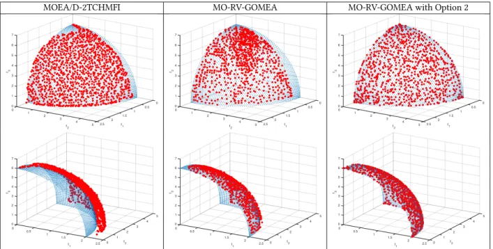
we can conclude that, in most cases, adaptation Option 2 is better than Option 1 for improving the performance of MO-RV-GOMEA. We hypothesize that a key factor in the outcomes is that removing checks for acceptance into the archive, which is expensive if the archive is full (1000 solutions), allows MO-RV-GOMEA with adap-tation Option 2 to perform many more evaluations (empirically we found up to a factor of 5). Note that the Tchebycheff scalarizations play a non-trivial role here, as simply removing the archive check in GOM in the original MO-RV-GOMEA deteriorates its performance. Figure 4 shows three approximation fronts with median IGD val-ues obtained by MOEA/D-2TCHMFI, the original MO-RV-GOMEA, and MO-RV-GOMEA with adaptation Option 2, respectively, for the WFG4 problem instance withm=3 objectives andl=320 decision variables. While the two MO-RV-GOMEAs both reach the reference front, there is still a considerable gap between the approximation front obtained by MOEA/D-2TCHMFI and the reference front. The
m WFG1 WFG2 WFG3 WFG4 2 0.1 1 10 0 100 200 300 400 500 600 700 MOEA/D-2TCHMFI MO-RV-GOMEA MO-RV-GOMEA with Option 1 MO-RV-GOMEA with Option 2
0.1 1 10 0 100 200 300 400 500 600 700 MOEA/D-2TCHMFI MO-RV-GOMEA MO-RV-GOMEA with Option 1 MO-RV-GOMEA with Option 2
0.1 1 10 0 100 200 300 400 500 600 700 MOEA/D-2TCHMFI MO-RV-GOMEA MO-RV-GOMEA with Option 1 MO-RV-GOMEA with Option 2
0.001 0.01 0.1 1 10 0 100 200 300 400 500 600 700 MOEA/D-2TCHMFI MO-RV-GOMEA MO-RV-GOMEA with Option 1 MO-RV-GOMEA with Option 2
10 1 10
0 500 1000 1500 2000 2500 3000 3500 MOEA/D-2TCHMFI
MO-RV-GOMEA MO-RV-GOMEA with Option 1 MO-RV-GOMEA with Option 2
1 10
0 500 1000 1500 2000 2500 3000 3500 MOEA/D-2TCHMFI
MO-RV-GOMEA MO-RV-GOMEA with Option 1 MO-RV-GOMEA with Option 2
0.1 1 10 0 500 1000 1500 2000 2500 3000 3500 MOEA/D-2TCHMFI MO-RV-GOMEA MO-RV-GOMEA with Option 1 MO-RV-GOMEA with Option 2
1 10 100 0 500 1000 1500 2000 2500 3000 3500 MOEA/D-2TCHMFI MO-RV-GOMEA MO-RV-GOMEA with Option 1 MO-RV-GOMEA with Option 2
Figure 3: The median IGD convergence on WFG1-4 problem instances with 320 variables. Horizonal axis: Time (seconds) in linear scale. Vertical axis: IGD in log scale. Some graphs might appear under another graph due to similar convergence.
MOEA/D-2TCHMFI MO-RV-GOMEA MO-RV-GOMEA with Option 2
0 0.5 0 1 0 2 1 3 1 f1 f3 4 5 1.5 2 f2 6 7 3 2 4 2.5 5 0 0.5 0 1 0 2 1 3 1 f1 f3 4 5 1.5 2 f2 6 7 3 2 4 2.5 5 0 0.5 0 1 0 2 1 3 1 f1 f3 4 5 1.5 2 f2 6 7 3 2 4 2.5 5 5 4 0 3 1 0 f2 2 0.5 2 3 f3 4 f1 1 5 1 1.5 6 7 2 2.5 0 5 4 0 3 1 0 f2 2 0.5 2 3 f3 4 f1 1 5 1 1.5 6 7 2 2.5 0 5 4 0 3 1 0 f2 2 0.5 2 3 f3 4 f1 1 5 1 1.5 6 7 2 2.5 0
Figure 4: Approximation fronts (in red) with the median IGD values on the WFG4 problem instance withm=3andl =320
(the reference Pareto-optimal fronts are in blue).
front obtained by MO-RV-GOMEA with adaptation Option 2 con-tains the extreme solutions and is more well-spread than the one of the original MO-RV-GOMEA.
The results presented above have been obtained by MO-RV-GOMEAs with the univariate model, i.e., all decision variables are considered as independent from each other. In MOEA/D-2TCHMFI, the polynomial mutation and simulated binary crossover (SBX) are employed to generate offspring solutions. While these two operators are also univariate, they still have certain differences
compared to the variation operator of MO-RV-GOMEAs. More detailed analysis would require experimenting with SBX in MO-RV-GOMEAs as well to recognize separately the contribution of scalarizations from the contribution of variation operators to the performance of MO-RV-GOMEAs compared to MOEA/D-2TCHMFI, which is outside the scope of this paper.
WFG2-3 are non-separable problems [11], i.e., their decision variables exhibit certain dependencies that need to be properly handled during solution variations so that the problem instances
Table 3: Results on solving WFG2-3 problems with MO-RV-GOMEAs using the linkage tree model.
l=40 l=80 l=160 l=320
m MOEA/D GOMEA Option 1 Option 2 MOEA/D GOMEA Option 1 Option 2 MOEA/D GOMEA Option 1 Option 2 MOEA/D GOMEA Option 1 Option 2
WFG2 2 0.009 (0.010) 0.001(0.001) 0.002 (0.001) 0.001 (0.000) 0.040 (0.182) 0.194 (0.193)0.001(0.002) 0.002 (0.193) 0.229 (0.019) 0.606 (0.413) 0.194 (0.413) 0.194 (0.413) 0.253 (0.019) 0.606 (0.000) 0.606 (0.413) 0.400 (0.413) 3 0.057 (0.014) 0.046 (0.015) 0.048 (0.013) 0.053 (0.018) 0.096 (0.071) 0.053 (0.023) 0.053 (0.014) 0.052 (0.013) 0.134 (0.173) 0.061 (0.027) 0.061 (0.023) 0.053 (0.184) 0.312 (0.037) 0.083 (0.180) 0.067 (0.190) 0.062 (0.238) 5 0.226 (0.037) 0.165(0.044) 0.180 (0.042) 0.198 (0.052) 0.236 (0.049) 0.184 (0.035) 0.182 (0.052) 0.182 (0.051) 0.276 (0.101) 0.217 (0.068) 0.204 (0.040) 0.179(0.032) 0.640 (0.389) 0.288 (0.085) 0.270 (0.049) 0.224(0.078) 10 0.793(0.484) 1.207 (0.763) 1.331 (0.528) 1.321 (0.928) 0.972 (0.886) 1.160 (0.911) 1.309 (1.097) 1.329 (0.796) 2.418 (0.686) 1.685 (0.682)1.447(0.926) 2.037 (0.264) 2.641 (0.688) 2.139 (0.434) 1.966 (0.490) 2.057 (0.308) WFG3 2 0.019 (0.014) 0.003 (0.002) 0.004 (0.001) 0.002 (0.001) 0.068 (0.034) 0.001 (0.000) 0.002 (0.006) 0.002 (0.001) 0.127 (0.033) 0.001 (0.000)0.001(0.000) 0.001 (0.001) 0.188 (0.022) 0.001(0.000) 0.001 (0.000) 0.001 (0.001) 3 0.100 (0.047) 0.031 (0.009) 0.034 (0.014) 0.026(0.007) 0.145 (0.061) 0.030 (0.012) 0.036 (0.008) 0.024(0.007) 0.193 (0.048) 0.034 (0.014) 0.037 (0.012) 0.022(0.010) 0.216 (0.055) 0.045 (0.038) 0.034 (0.013) 0.021(0.009) 5 0.261 (0.161) 0.199 (0.066) 0.177 (0.104) 0.124(0.053) 0.414 (0.210) 0.171 (0.068) 0.164 (0.128) 0.102(0.030) 0.485 (0.153) 0.146 (0.043) 0.158 (0.092) 0.094(0.043) 0.470 (0.174) 0.173 (0.095) 0.153 (0.058) 0.080(0.036) 10 0.810 (0.165) 0.401 (0.195) 0.329 (0.283) 0.187(0.085) 0.819 (0.141) 0.342 (0.265) 0.384 (0.507) 0.216(0.136) 0.807 (0.100) 0.359 (0.272) 0.235 (0.184) 0.228 (0.064) 0.786 (0.133) 0.326 (0.269) 0.317 (0.401) 0.190(0.080)
can be efficiently solved. Table 3 shows the medians and the in-derdecile ranges of the IGD metric of the approximation fronts obtained by the three MO-RV-GOMEA variants that employ the linkage tree model, which is learned over the selection of solu-tions in each generation to capture the linkage structures, and the MOEA/D-2TCHMFI. We do not implement the linkage tree model for MOEA/D-2TCHMFI because non-trivial modifications would be required for MOEA/D-2TCHMFI (which, by default, creates a whole offspring solution each time) to make use of the linkage tree. In most cases, MO-RV-GOMEAs with the linkage tree model obtain better IGD values compared to the ones with the univari-ate model (i.e., compare Table 2 and Table 3). For WFG2 problem instances withl=80,160,320 variables, the two adapted
MO-RV-GOMEAs achieve better approximation fronts than the original MO-RV-GOMEA and MOEA/D-2TCHMFI. For WFG3 problem in-stances, MO-RV-GOMEA with Option 2 almost always outperforms other MOEAs. A more detailed analysis on the effect of linkage learning (for such large problem instances) requires more computa-tion time and thus is left for future work.
6
CONCLUSIONS
We investigated the performance of the MO-RV-GOMEA on a wide range of multi-objective and many-objective benchmark problems. The experimental results indicate that MO-RV-GOMEA is quite well-suited also for solving many-objective problems without requiring any modification, unlike many other MOEAs that are designed on the basis of multi-objective optimization. For some benchmark problems, the performance of MO-RV-GOMEA can be further im-proved when the improvement checks during solution variation are guided by carefully constructed Tchebycheff scalarizations. Per-formance comparisons with a state-of-the-art decomposition-based MOEA (i.e., MOEA/D-2TCHMFI) show that both the original and adapted MO-RV-GOMEAs are the preferred algorithms of choice for tackling (real-world) problems that require many conflicting objectives to be optimized at the same time.
ACKNOWLEDGMENTS
This work is part of the research programme IPPSI-TA with project number 628.006.003, which is financed by the Netherlands Organi-sation for Scientific Research (NWO) and Elekta.
REFERENCES
[1] M. Asafuddoula, Tapabrata Ray, and Ruhul Sarker. 2015. A decomposition-based evolutionary algorithm for many objective optimization.IEEE Transactions on Evolutionary Computation19, 3 (2015), 445ś460.
[2] Leonardo C. T. Bezerra, Manuel López-Ibáñez, and Thomas Stützle. 2016. A perfor-mance assessment of tuned multi- and many-objective evolutionary algorithms. (2016). http://iridia.ulb.ac.be/supp/IridiaSupp2015-007/.
[3] Peter A.N. Bosman and Dirk Thierens. 2002. Multi-objective optimization with diversity preserving mixture-based iterated density estimation evolutionary algorithms.International Journal of Approximate Reasoning31, 3 (2002), 259ś289. [4] Peter A. N. Bosman. 2010. The anticipated mean shift and cluster registration
in mixture-based EDAs for multi-objective optimization. InProceedings of the Genetic and Evolutionary Computation Conference - GECCO 2010. ACM Press, New York, New York, USA, 351ś358.
[5] Peter A. N. Bosman and Marcus Gallagher. 2016. The importance of implementa-tion details and parameter settings in black-box optimizaimplementa-tion: a case study on Gaussian estimation-of-distribution algorithms and circles-in-a-square packing problems.Soft Computing(2016), 1ś15.
[6] Anton Bouter, Ngoc Hoang Luong, Cees Witteveen, Tanja Alderliesten, and Peter A. N. Bosman. 2017. The multi-objective real-valued gene-pool optimal mixing evolutionary algorithm. InProceedings of the Genetic and Evolutionary Computation Conference - GECCO 2017. 537ś544.
[7] Indraneel Das and John E. Dennis. 1997. A closer look at drawbacks of minimizing weighted sums of objectives for Pareto set generation in multicriteria optimization problems.Structural Optimization14, 1 (1997), 63ś69.
[8] Indraneel Das and John E. Dennis. 1998. Normal-Boundary Intersection: a new method for generating the Pareto surface in nonlinear multicriteria optimization problems.SIAM Journal on Optimization8, 3 (1998), 631ś657.
[9] Kalyanmoy Deb and Himanshu Jain. 2014. An evolutionary many-objective opti-mization algorithm using reference-point-based nondominated sorting approach, Part I: solving problems with box constraints.IEEE Transactions on Evolutionary Computation18, 4 (2014), 577ś601.
[10] Kalyanmoy Deb, Lothar Thiele, Marco Laumanns, and Eckart Zitzler. 2005. Scal-able Test Problems for Evolutionary Multiobjective Optimization. InEvolutionary Multiobjective Optimization. Springer-Verlag, London, 105ś145.
[11] Simon Huband, Phil Hingston, Luigi Barone, and Lyndon While. 2006. A review of multiobjective test problems and a scalable test problem toolkit.IEEE Transactions on Evolutionary Computation10, 5 (2006), 477ś506.
[12] Hisao Ishibuchi, Ken Doi, and Yusuke Nojima. 2016. Characteristics of many-objective test problems and penalty parameter specification in MOEA/D. In2016 IEEE Congress on Evolutionary Computation (CEC). IEEE, 1115ś1122. [13] Joshua Knowles and David Corne. 2003. Properties of an adaptive archiving
algorithm for storing nondominated vectors.IEEE Transactions on Evolutionary Computation7, 2 (2003), 100ś116.
[14] Ke Li, Kalyanmoy Deb, Qingfu Zhang, and Sam Kwong. 2015. An evolutionary many-objective optimization algorithm based on dominance and decomposition.
IEEE Transactions on Evolutionary Computation19, 5 (2015), 694ś716. [15] Fernando G. Lobo and David E. Goldberg. 2004. The parameter-less genetic
algorithm in practice.Information Sciences167, 1 (2004), 217ś232.
[16] Ngoc Hoang Luong, Tanja Alderliesten, Arjan Bel, Yury Niatsetski, and Peter A.N. Bosman. 2017. Application and benchmarking of multi-objective evolutionary algorithms on high-dose-rate brachytherapy planning for prostate cancer treat-ment.Swarm and Evolutionary Computation(2017). https://doi.org/10.1016/j. swevo.2017.12.003
[17] Ngoc Hoang Luong and Peter A. N. Bosman. 2012. Elitist archiving for multi-objective evolutionary algorithms: to adapt or not to adapt. InParallel Problem Solving from Nature - PPSN XII, Vol. 7492. Springer Berlin Heidelberg, 72ś81. [18] Xiaoliang Ma, Qingfu Zhang, Junshan Yang, and Zexuan Zhu. 2017. On
Tcheby-cheff decomposition approaches for multi-objective evolutionary optimization.
IEEE Transactions on Evolutionary Computation(2017), 1ś20.
[19] Qingfu Zhang and Hui Li. 2007. MOEA/D: A multiobjective evolutionary algo-rithm based on decomposition.IEEE Transactions on Evolutionary Computation
11, 6 (2007), 712ś731.
[20] Dirk Thierens and Peter A. N. Bosman. 2011. Optimal mixing evolutionary algorithms. InProceedings of the Genetic and Evolutionary Computation Conference - GECCO 2011. ACM Press, New York, New York, USA, 617ś624.
[21] Ye Tian, Ran Cheng, Xingyi Zhang, and Yaochu Jin. 2017. PlatEMO: A MATLAB platform for evolutionary multi-objective optimization [Educational Forum].
IEEE Computational Intelligence Magazine12, 4 (2017), 73ś87.
[22] Anupam Trivedi, Dipti Srinivasan, Krishnendu Sanyal, and Abhiroop Ghosh. 2017. A survey of multiobjective evolutionary algorithms based on decomposition.IEEE Transactions on Evolutionary Computation21, 3 (2017), 440ś462.