37
Multiclass Sequential Feature Selection and Classification Method
for Genomic Data
W. B. Yahya G. T. Aremu M. K. Garba
Department of Statistics, Faculty of Physical Sciences, University of Ilorin, Ilorin, Nigeria
Abstract
This paper presents an efficient multiclass sequential feature selection and classification (mk-SS) method using gene expression signatures. The development of this method employs 10-fold cross-validation to ensure stability. The efficiency of this method is assessed through the misclassification error rate and some other performance measures. The performances of the mk-SS were compared with the classification results of the Support Vector Machines (SVM) over five published multiclass microarray datasets. The results showed that the mk-SS method efficiently selects the informative gene biomarkers for proper classification of the biological groups of the tissue samples. This method competes favourably with SVM in terms of prediction accuracy while it outperforms the SVM in 80% of cases considered. The quality of the features selected by mk-SS algorithm was validated by hybridizing the feature selection scheme of the mk-SS into the standard SVM algorithm which significantly improves the predictive power of the standard SVM method. This work has shown that classification of various cancer type using gene expression profiles is feasible especially when the endpoints are of multi-category.
Keywords: k-SS, mk-SS, Support Vector Machines, Microarray, Misclassification error rate
1. Introduction
Non-clinical classification of cancer tumour samples using gene expression profiles has been given prominent attention in the recent time (Harper, 2005; Theisen et al, 2006; Yahya et al, 2014). Attention has been more on binary class prediction than the multiclass cases (Yahya et al, 2011; Hapfelmeier et al., 2011). However, the situations that call for multiclass tissue sample classification are becoming more frequent in many clinical studies (Perou et al., 2000; Ramaswamy et al., 2001; Beer et al., 2002). Thus, the need for the development of more efficient methods for the classification of biological samples using gene expression data for multi-category response groups is inevitable.
An early diagnosis of a disease or tumourous patients will enable easy identification of disease status and increase the patients’ survival rate (Yahya and Ulm, 2009). Literature has it that clinical diagnosis of cancer tumour might take considerable longer time before proper identification could take place (Yahya et al, 2014). Within such period, the cancer tumour might metastasize which may eventually affect the survival of the patients. An alternative non-clinical approach is the use of microarray technology for proper cancer diagnosis using the gene expression profiles (Burnside et al , 2008; Cooper, 2001; Surks et al, 2003; Ochs and Godwin, 2004)
In this paper, two non-clinical methods for multi-category cancer tumour classification using high-dimensional microarray data sets are compared. These are the multiclass sequential feature selection and classification (mk-SS) method and the support vector machines (SVM). The efficiency of the methods relative to each other was reported in terms of their classification results and identification of relevant gene biomarkers.
2.0 Materials and Method
2.1 Data Descriptions
Five different published data sets were employed to demonstrate the applications of the mk-SS and the SVM for tissue sample classification and feature selection in this work. All the five data sets are multi-categorical response microarray cancer data sets.
A short description of the five data sets employed here is provided in what follows.
The first data set was the Small Round Blue-Cell Tumor (SRBCT) data of childhood described by Khan et al. (2001). The data contained four different types of tumors with 11, 29, 18 and 25 biological samples in the four tumour groups. By this, a total of 83 biological samples and 2,308 gene chips were present in the data.
The second data consist of consist of four distinct types of Thyroid tumor cells. For each tissue sample, 2,000 gene expression measurements were available. As described in James et al.(2013), the four tumour classes in the data were coded as "FA"=1, "FC"=2, "N"=3 and "PC"=4 which correspond to the four biological groups with respective sample sizes 17, 8, 12 and 12.
The next data set was microarray breast cancer data with five distinct cancer tumour subtypes. The data contained a total of 85 biological samples on which 456 gene expression profiles were measured. The sub-group sample sizes were 14, 11, 13, 15 and 32 as described in Sørliea et al. (2001and 2003). These data can be accessed at http://genome-www.stanford.edu/breast_cancer/.
The fourth data set called the ‘Christensen data’ is a microarray data set that contained 1,414 gene expression profiles of 217 tissue samples with three distinct sub-tumour groups. The three response groups were coded as
38
"Blood" = 1 and "Placenta" = 2, "Others" = 3. These data are pre-loaded in the R statistical package and can be accessed through the URL site http://www.R-project.org/
The last data set analysed in this work contained gene expression profiles of nine cancer subtype as described in Ross et al.(2000). The nine tumour classes were coded as "BREAST" = 1, "CNS" = 2, "COLON" = 3, "LEUKEMIA" = 4, "MELAN" = 5, "NSCLC" = 6, "OVARY" = 7, "PROSTRATE" = 8 and "RENAL" = 9. These data are available online and can be accessed at: http://genome-www.stanford.edu/nci60/help.shtml.
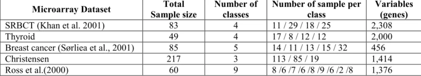
The characteristics of the five published data sets used in this work are presented in Table 1 for clarity.
Table 1: Summary of the characteristics of the five published datasets used
Microarray Dataset Total
Sample size
Number of classes
Number of sample per class
Variables (genes)
SRBCT (Khan et al. 2001) 83 4 11 / 29 / 18 / 25 2,308
Thyroid 49 4 17 / 8 / 12 / 12 2,000
Breast cancer (Sørliea et al., 2001) 85 5 14 / 11 / 13 / 15 / 32 456
Christensen 217 3 113 / 85 / 19 1,414
Ross et al.(2000) 60 9 8 /6 /7 /6 /8 /9 /6 /2 /8 1,376
2.2 Multiclass Classification Techniques
Multiclass learning simply implies learning to classify an object into one of many classes other than binary. However, this extension is not straight forward in some cases.
This method focuses on effective identification of informative genes for each group. Feature selection is very important for biomarker discovery in microarray experiment and this leads to new knowledge about the biology of the disease. In that case, the genes selected are more important than the classifier used.
A number of methods to handle the classification of multi-categorical responses using genomic data have been reported in the literature. Notable among these are the Decision Tree (DT) algorithm (Quinlan, 1993), Classification and Regression Trees (CART) (Breiman, 1993; Breiman, 2001), Random forest (RF) classifiers (Breiman, 2001; Hapfelmeier, 2012) and the like.
The first step in multiclass classification using microarray data is to form the pivot category. This is the formation of subpopulations of binary response groups with identical covariate patterns. At this stage, the scheme to adopt to form the series of binary subgroups from the original multi-categories of the tissue samples is determined. Two of the popular approaches to handle this are the pear-wise coupling (Hastie and Tibshirani, 1998; Hastie et al., 2001; Tan et al., 2005) and One-versus-Others schemes (Hand, 1997; Speed, 2003; Dudoit et al., 2002). The pear-wise coupling technique is sometimes referred to as One-versus-One scheme (Tan et al., 2005) or Round Robin Ensemble (Furnkranz, 2002). In this work, the scheme of One-versus-Others which is sometimes called One-against-All (Aremu and Yahya, 2015) is employed for the two classifiers discussed here.
As a brief overview of One-versus-Others, consider a polytomous response class = 0, 1, … , in which the class members follow some natural ordering, the classifier can be constructed to distinguish a reference class ∗∈ from all other class labels. By this, all other complementary classes are put into one group and subgroups of binary responses are formed with the existing set of gene predictors.
Specifically, in a multiclass microarray classification problem with three distinct biological groups defined by = 1 ℎ 1 2 ℎ 2 3 ℎ 3 , (1)
the One-versus-Others scheme requires that the following three possible binary data subgroups be formed and used for classification using the set of gene signatures: = #1 ℎ 0 ℎ 2 3 1 (2)
= #1 ℎ 0 ℎ 1 3 2 (3)
= #1 ℎ 0 ℎ 1 2 3 (4)
The final performance of a classifier is however based on majority votes after classification results are obtained (Hand, 1997; Speed, 2003; Dudoit et al., 2002).
The above procedure can be easily extended for multiclass problems with more than three biological groups. 2.3 The Multiclass k - Sequential Feature Selection and Classification (mk-SS) Method
39
k-Sequential feature Selection and classification (k-SS) method for binary class microarray data problem (Yahya, 2009; Yahya et al., 2011; Hapfelmeier et al., 2012; Yahya, 2012; Yahya et al., 2014). The classical k-SS classifier provides a fast and flexible algorithm that sequentially selects relevant features for classification in any binary response microarray classification problems. It is a stepwise feature selection that adopt misclassification error rate (MER) as the search criterion.
The mk-SS method allows the choice of classes of outcome to be modeled as a set of independent binary outcomes in which − 1 classes are chosen as a "pivot" class (one set of pivot classes at a time) and this is combined with the remaining one class of outcome for feature selection and classification. The log of the ratio of the posterior probabilities used in the logit function employed by the mk-SS classifier would be of the form
% &'( = )∑/01*+ ∗,*+ ,'-'
-2 3 following the classical binary class set-up in equations (2) to (4).
2.3.1 The mk-SS Algorithm in Brief
Step1: Based on the binary class settings in Section 2.2, logit model of the form % +45- = 67+45-8 = 9 +
;545, = 1, … , is fitted to on individual gene variable 45 using the training sample < and compute the misclassification error rates (MERs), =>5=@?
AB∑
C
= 1 DEFGH+IJ-KLHM for each 45 over the test sample C, where
E&.(= 1 if the argument is true and 0 otherwise. Within the logistic regression set up, the predicted class label
%O +45- = O = 1 if &O = 1|45( ≥ 0.5 and O = 0 if otherwise.
Step2: Randomly draw R replicates of training sample < with or without replacement (depending on the
cross-validation type adopted), from the original sample and compute the average MERs =̅>5= ?
T×@AB∑ V= 1∑
C
= 1 DEFGHW+IJ-KLHWM for each gene 45, = 1, … , .
Step3: Selectthe gene variable 4&?( that yields the least average MER value, say =̅>&?( among all the MER values
=̅>5, = 1, … , in STEP 2.
Step4: The second best gene predictor 4&X( is selected by forming a set of pairs of genes with the first selected
gene 4&?( and the remaining − 1 left out genes. Repeat steps 1 and 2 on each of the gene pairs and the gene pair
4&?(4&X( that yielded the least average MER, say =̅>&X( is selected.
Step5: Before the third best gene 4&Y(, and more generally, the &Z + 1( best gene 4&[\?( could be selected after the selection of the Z gene 4&[(, the marginal gain in prediction strength ∆^[= =̅>&[(− =̅>&[\?( due to the inclusion of gene 4&[( into the classification model is examined by testing the hypothesis H0k: ∆[= 0 vs. H1k: ∆[> 0, ∆[=
=̅&[(− =̅&[\?( , via the test statistic
`∆^a=
∆^abc&∆^a(
de&∆^a(
where f&∆^[( is the empirical variance and `∆^a has a skew-normal density with shape parameter g = 4.0398 (Yahya et al., 2011) where k+∆^[- = 0 under H0k.
Decision rule:
i.) When the null hypothesis H0k cannot be rejected, then, the &Z + 1( gene 4&[\?( under consideration is dropped from the classification model and the k-SS algorithm terminates assuming that no other gene variable among the remaining − Z genes is capable of improving the prediction strength of the current classification model containing Z gene variables.
ii.) If H0k is rejected, it shows that gene 4&[\?( has significantly enhanced the prediction strength of the current classification model and should therefore be retained while the selection of the next best gene 4&[\X( begins following Steps 1 to 4.
Repeat Steps 1 to 5 until no more gene satisfies the decision rule ii. above. STOP and RETURN the selected k genes.
2.4 Support Vector Machines
Support vector machines (SVM) is one of the state-of-the art techniques developed in the field of statistical learning theory and pattern recognition (Vapnik and Chervonenkis, 1974; Vapnik, 1982; 1995; 1998). The SVM method has become increasingly popular among the kernel based methods as an excellent tool in response group classification, regression and statistical pattern recognition (Cortes and Vapnik, 1995; Lee, 2004; Yahya, 2012). The goal in SVM methods (Smola and Schoelkopf, 2004; Yahya, 2012) is to find a decision function of the form ℎ&l( = &〈n. l〉 + ( (5)
40
with Euclidean norm ‖n‖ = 〈n. n〉?/X= 1 with being the bias. The quantity 〈n. l〉 is the inner product of vectors nand l defined as 〈n. l〉 = nrl.
Suppose we define a hyperplane st∈ s, simply called the separating hyperplane, that separates the training samples into the two existing response class labels &−1,1(. If the two response groups in the training sample are linearly separable, then the maximal distance of the separating hyperplane st from the closest positive sample ( = 1) can be defined by u\ units and its respective maximal distance from the closest negative sample & =
−1( by ub units. If the two maximal distances are the same, that is, u\= ub= u, then the two sample groups are 2u units apart. The task in SVM procedure therefore, is to find the weight vector n and bias that will maximize the distance u.
In a linearly separable sample, the SVM algorithm seeks for the separating hyperplane with the maximal margin (distance) u. This essentially results to the following optimization problem using (5);
vwx
n,y u (6) subject to the conditions that;
〈n. l〉 + ≥ u, if = 1 (7) 〈n. l〉 + ≤ −u, if = −1 (8)
with nhaving a unit norm ‖n‖ = 1. Therefore, for any given linearly separable set of training data, we define a maximal margin hyperplane s?∈ s for which the equality 〈n. l〉 + = u in (7) holds and maximal margin hyperplane sb?∈ s for which the equality 〈n. l〉 + = −u in (8) also holds. The vector l of gene variables for which these two equalities are satisfied is called support vector and the solutions of the optimization problem depend only on this vector and not on the entire dimension of the training set (Bennett and Campbell, 2000). The goodness of SVM classifier ℎ&x ( is determined through the average MER over the test sample C defined by
=̅>{|}=X@?
AB∑ , − ℎ^&x (,
@AB
~? (9)
where ∈ &−1,1( is the observed class labels and ℎ^&x ( ∈ &−1,1( is the predicted class label of the classifier
ℎ&x ( for subject.
3.0 Analysis and Results
The mk-SS and SVM methods were implemented on the five published microarray data sets described in Section 2.1 following their procedures as detailed in Section 2. The 10-fold cross-validation technique (Yahya, 2012) was employed in which the entire sample data is randomly partitioned into ten segments of apparently equal lengths and nine of such segments were used to train the two classifiers and the samples in the tenth segment were used as the training data to assess their performances. This was repeated ten times to ensure that each data segment is used as training and test sets at different times to ensure results’ stability. The performances of the classifiers were assessed through the average misclassification error rate (MER) or average correct classification rate (CCR). All analyses were implemented in the environment of R statistical package (http://www.R-project.org).
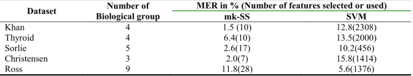
Table 2: Table of the Misclassification Error Rates (MERs in %) provided by mk-SS and SVM on the five cancer
microarray data sets. The numbers of features employed for classification by the two methods are equally reported in parentheses as well as number of groups of biological sample in each data.
Dataset Number of
Biological group
MER in % (Number of features selected or used)
mk-SS SVM Khan 4 1.5 (10) 12.8(2308) Thyroid 4 6.4(10) 13.5(2000) Sorlie 5 2.6(17) 10.2(456) Christensen 3 2.0(7) 15.8(1414) Ross 9 11.8(28) 5.6(1376)
41
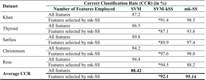
Table 3: Table of classification results of mk-SS and SVM classifier on all the five published data sets considered.
The Correct Classification Rate (CCR) (in %) provided by the two methods were reported. Results of the SVM that employed only the selected features by mk-SS algorithm here called the SVM-kSS classifier are equally reported as asterisked (*) for easy comparisons.
Dataset Correct Classification Rate (CCR) (in %)
Number of Features Employed SVM SVM-kSS mk-SS
Khan All features 87.2
Features selected by mk-SS *91.4 98.5
Thyroid All features 86.5
Features selected by mk-SS *87.1 93.6
Sørliea All features 89.8
Features selected by mk-SS *89.9 97.4
Christensen All features 84.2
Features selected by mk-SS *97.6 98.0
Ross All features 94.4
Features selected by mk-SS *94.5 88.2
Average CCR All features 88.42
Features selected by mk-SS *92.1 95.14
We present in Table 2, the estimated average MERs (in %) provided by the mk-SS and SVM classifiers on the five published data sets over the test samples. The number of response class (biological groups) in each data as well as the number of genes employed for classification (in parentheses) that yielded the respective (MERs) performances by each method is reported. The numbers of genes reported against the MERs for mk-SS method were the numbers of genes selected by the mk-SS algorithm for classification. On the other hand, the numbers of genes reported for SVM were the entire gene variable in the respective data sets as earlier stated in Section 2.
In Table 3, the CCRs (in %) yielded by mk-SS and SVM classifiers over all the five published data sets are presented. The results of the SVM that employed only the selected genes by the mk-SS algorithm which is here called the SVM-kSS classifier are equally reported in the table.
Fig 1: Line graphs of estimated correct classification rates (CCR) (in %) of mk-SS, SVM, and SVM-kSS
classifiers for all the five published data sets. The SVM-kSS classifier is the SVM classifier that employed only the features selected by mk-SS algorithms as its input gene predictors. The SVM classifier used all the available
features in each data set for classification.
4.0 Discussion and Conclusion
Another variant of feature selection and classification technique, mk-SS for multiclass microarray data problem is presented in this work. It incorporates the features of the classical k-SS method (Yahya, 2012; Hapfelmeier et al., 2012; Yahya et al, 2014) for binary class data problems.
Results in Table 1 showed that the prediction accuracy of mk-SS method is better than that of the SVM
Khan Thyroid Sørliea Christensen Ross
SVM 87.2 86.5 89.8 84.2 94.4 SVM-kSS 91.4 87.1 89.9 97.9 94.5 mk-SS 98.5 93.6 97.4 98 88.2 75 80 85 90 95 100 C C R ( in % )
42
in four of the five data sets considered. The prediction performance mk-SS method is slightly lower than that of SVM in just one of the cases (Ross data set). By this, it showed that the mk-SS is relatively more efficient in 80% of the cases than the SVM classifier. However, if we consider the average overall prediction performances of the two classifiers reported in Table 3, it can be easily observe that the mk-SS classifier with overall prediction accuracy of about 95% performs better than SVM that yielded about 88% prediction accuracy.
It should be noted that while the SVM method uses all the gene predictors that are available in the various data sets for classification, the mk-SS method efficiently selected only few relevant gene subsets from these pool to achieve better classification results. The numbers of genes selected by the mk-SS method to achieve the respective prediction accuracies are provided in parentheses in Table 1 for all the data sets.
It can be observed that can be observed from the results in Table 1 that the number of genes employed by mk-SS to achieve good prediction accuracies are relatively fewer than that of SVM that uses all the gene variables in the data. This is a simple indication that the genes selected for classification by mk-SS methods are quite relevant and more correlated to the respective biological groups in the data sets.
To further demonstrate the quality of genes selected by mk-SS method for tumour classification, the techniques of both the mk-SS and SVM were hybridized which resulted into SVM-kSS classifier. By this hybridized procedure, the few marker genes selected by mk-SS algorithm in all the five genomic data sets were fed into the SVM algorithm for classification. The results in Table 3 showed that the prediction accuracies of the SVM-kSS method (that employed the genes selected by mk-SS) are far better than that of the traditional SVM method in all the five data sets. These various performances of all the classifiers are clearly presented by the line graphs in Fig 1 across the five microarray data sets.
This work has shown that classification of various cancer type using gene expression profiles is feasible especially when the cancer type are of multi-category. The performance measures adopted show the efficiency of the mk-SS method as compared to SVM classifier on multiclass response groups. However, further validation regarding the efficiency of the proposed mk-SS method for multiclass prediction might be desirable in future, especially on microarray data sets with complex structures. This will enable a broader comparison of its prediction performance with several other existing competing algorithms for multiclass tumour classification.
References
[1] Aremu GT & Yahya WB (2015): Competing Algorithms For Microarray-Based Multiclass Sequential Feature Selection and Classification. Proceedings of 4th International Science, Technology, Education,
Arts, Management & Social Sciences (iSTEAMS) Research Nexus Conference.
[2] Beer DG et al. (2002): Gene-expression profiles predict survival of patients with lung adenocacinoma. Nat. Med., 8: 816-824.
[3] Bennett KP & Campbell C (2000): Support vector machines: Hype of Hallelujah? SIGKDD Explorations,
2(2): 1-13.
[4] Breiman L (1993): Better subset selection using the non-negative garrotte. Technical Report, University of California, Berkeley (1993).
[5] Breiman L (2001): Random forests. Machine Learning, 45(1):5–32, 2001. ISSN 08856125. doi:10.1023/A:1010933404324. URL: http://dx.doi.org/10.1023/A: 1010933404324.
[6] Burnside J, Ouyang M, Anderson A, Bernberg E, Lu C, Meyers BC, et al. (2008): Deep sequencing of chicken microRNAs. BMC Genomics, 9:185
[7] Cooper CS (2001): Applications of microarray technology in breast cancer research. Breast Cancer Research, 3:158-71.
[8] Cortes C & Vapnik VN (1995): Support vector networks. Machine Learning, 20:273–297.
[9] Dudoit S, Fridlyand J & Speed TP (2002): Comparison of discriminant methods for the classification of tumors using gene expression data. Jour. Amer. Stat. Assoc., 97: 77-87.
[10] Furnkranz J (2002): Round Robin Classification. Journal of Machine Learning Research, 2: 721-747. [11] Hand DJ (1997): Construction and assessment of classification rules. John Wiley & Sons, New York. [12] HapfelmeierA (2012): Random Forest variable importance with missing data. Technical report 121,
Institute for Statistics, LMU Munich, http://www.stat.uni-muenchen.de
[13] HapfelmeierA, Yahya WB, Rosenberg R & Ulm K. (2012): Predictive modelling of gene Expression data. In: Handbook of Statistics in Clinical Oncology, 3rd ed., Edited by Crowley, J. and A. Hoering. Chapman and Hall/CRC, New York, pp: 463-475.
[14] Harper PR (2005): A review and comparison of classification algorithms for medical decision making. Health Policy, 71(3): 315-31.
[15] Hastie T and Tibshirani R (1998): Classification by pair-wise coupling. Annals of statistics, 26(2): 451-471.
[16] Hastie T, Tibshirani R and Friedman J (2001). The Elements of Statistical learning, Springer.
43 Applications in R. Springer-Verlag, New York.
[18] Khan et al (2001): Classification and diagnostic prediction of cancers using gene expression profiling and artificial neural networks. Nat. Med., 7(6):673 - 679.
[19] Lee M-LT (2004): Analysis of microarray gene expression data. Springer, New York.
[20] Ochs MFand Godwin AK (2004): Microarrays in cancer: research and applications. BioTechniques. Suppl.: 4-15.
[21] Perou CM, Sùrlie T, Eisen MB et al. (2000): Molecular portraits of human breast tumours. Nature, 406.17: 747-752.
[22] Quinlan JR (1993): Programs for Machine Learning. Morgan Kaufmann Publishers, Inc., NY.
[23] Ramaswamy S, Tamayo P, Rifkin R et al. (2001): Multiclass cancer diagnosis using tumor gene expression signatures. Proc. Natl. Acad. Sci. USA, 98.26: 15149–15154.
[24] Ross DT1., Scherf U, Eisen MB, Perou CM. Christian R.(2000): Systematic variation in gene expression patterns in human cancer cell lines. Nat. Genet.;24(3):227-35
[25] Smola AJ & Schoelkopf B, (2004): A tutorial on support vector regression. Statistics and Computing, 14: 199-222.
[26] Sørliea T, Peroua CM, Tibshirani R, Aasf T, Geislerg S, Johnsenb H, Hastiee T, Eisenh MB, van de Rijni M, Jeffreyj SS, Thorsenk T, Quistl H, Matesec JC, Brownm PO, Botsteinc D, Lønning PE & Børresen-Daleb A-L (2001): Gene expression patterns of breast carcinomas distinguish tumor subclasses with clinical implications. Proc. Natl. Acad. Sci. USA, 98(19): 10869 – 10874
[27] Sørliea T, Tibshirani R, Parker J, Hastie T, Marron JS, Nobel A, Deng S, Johnsen H, Pesich R, Geisler S, Demeter J, Perou CM, Lønning PE, Brown PO, Børresen-Dale A-L & Botstein D (2003): Repeated observation of breast tumour subtypes in independent gene expression datasets.Proc. Natl. Acad. Sci. USA, 100 (14) 8418-8423; doi:10.1073/pnas.0932692100
[28] Speed T (2003): Statistical analysis of gene expression microarray data. Chapman & Hall, London. [29] Surks HK, Richards CT & Mendelsohn ME. (2003): Myosin phosphatase-Rho interacting protein. A new
member of the myosin phosphatase complex that directly binds RhoA. J. Biol. Chem., 278(51): 51484-93.
[30] Tan AC, Naiman DQ, Xu L, Winslow RL & Geman D (2005): Simple decision rules for classifying human cancers from gene expression profiles. Bioinformatics, 21(20): 3896-3904.
[31] Theisen J, Kauer WK-H, Nekarda H, Schmid L, Stein HJ & Siewert J-R (2006): Neoadjuvant Radiochemotherapy for Patients with Locally Advanced Rectal Cancer leads to Impairment of the Anal Sphincter. Journal of Gastrointestinal Surgery, 10(2): 309-314.
[32] Vapnik VN (1982): Estimation of Dependences Based on Empirical Data. Springer, Berlin. [33] Vapnik VN (1995): The Nature of Statistical Learning Theory. Springer, New York. [34] Vapnik VN (1998): Statistical Learning Theory . John Wiley and Sons, New York.
[35] Vapnik VN & Chervonenkis A (1974): Theory of Pattern Recognition (in Russian). Nauka, Moscow (German Translation: W. Wapnik & A. Tscherwonenkis, Theorie der Zeichenerkennung. 1979, Akademie-Verlag, Berlin).
[36] Vapnik VN & Lerner, (1963): A Pattern recognition using generalized portrait method. Automation and Remote Control, 24: 774–780.
[37] Yahya WB (2009): Sequential dimension reduction and prediction methods with high dimensional microarray data. Universitätsbibliothek, Ludwig- Maximilians-Universität, München, Germany. Ph.D. Thesis. URL: http://edoc.ub.uni-muenchen.de/10254/
[38] Yahya WB (2012), Genes selection and tumour classification in cancer research: A new approach. Lambert Academic Publishing, Säbruck, Germany.
[39] Yahya WB & Ulm K (2009): Survival analysis of breast and small-cell lung cancer patients using conditional logistic regression models. International Journal of Ecological Economics & Statistics 14(S09): 15-35.
[40] Yahya WB, Rosenberg R & Ulm K (2014): Microarray-based Classification of Histopathologic Responses of Locally Advanced Rectal Carcinomas To Neoadjuvant Radiochemotherapy Treatment. Turkiye Klinikleri Journal of Biostatistics, 6(1):8-23.
[41] Yahya WB, Ulm K, Ludwig F & Hapflemeir A, (2011): K-SS: A sequential feature selection and prediction method in microarray study. International Journal of artificial intelligence, Spring , volume 6, number S11.