Sorting
8
T
HIS CHAPTERstudies several important methods for sorting lists, both
con-tiguous lists and linked lists. At the same time, we shall develop further
tools that help with the analysis of algorithms and apply these to determine
which sorting methods perform better under different circumstances.
8.1 Introduction and Notation 318
8.1.1 Sortable Lists 319 8.2 Insertion Sort 320 8.2.1 Ordered Insertion 320 8.2.2 Sorting by Insertion 321 8.2.3 Linked Version 323 8.2.4 Analysis 325 8.3 Selection Sort 329 8.3.1 The Algorithm 329 8.3.2 Contiguous Implementation 330 8.3.3 Analysis 331 8.3.4 Comparisons 332 8.4 Shell Sort 333 8.5 Lower Bounds 336 8.6 Divide-and-Conquer Sorting 339
8.6.1 The Main Ideas 339 8.6.2 An Example 340
8.7 Mergesort for Linked Lists 344
8.7.1 The Functions 345
8.7.2 Analysis of Mergesort 348
8.8 Quicksort for Contiguous Lists 352
8.8.1 The Main Function 352 8.8.2 Partitioning the List 353 8.8.3 Analysis of Quicksort 356
8.8.4 Average-Case Analysis of Quicksort 358 8.8.5 Comparison with Mergesort 360
8.9 Heaps and Heapsort 363
8.9.1 Two-Way Trees as Lists 363 8.9.2 Development of Heapsort 365 8.9.3 Analysis of Heapsort 368 8.9.4 Priority Queues 369
8.10 Review: Comparison of Methods 372
Pointers and Pitfalls 375
Review Questions 376
References for Further Study 377
We live in a world obsessed with keeping information, and to find it, we must keep it in some sensible order. Librarians make sure that no one misplaces a book; income tax authorities trace down every dollar we earn; credit bureaus keep track of almost every detail of our actions. I once saw a cartoon in which a keen filing clerk, anxious to impress the boss, said frenetically, “Let me make sure these files are in alphabetical order before we throw them out.” If we are to be the masters of this explosion instead of its victims, we had best learn how to keep track of it all!
Several years ago, it was estimated, more than half the time on many com-practical importance
mercial computers was spent in sorting. This is perhaps no longer true, since sophisticated methods have been devised for organizing data, methods that do not require that the data be kept in any special order. Eventually, nonetheless, the 249
information does go out to people, and then it must often be sorted in some way. Because sorting is so important, a great many algorithms have been devised for doing it. In fact, so many good ideas appear in sorting methods that an entire course could easily be built around this one theme. Amongst the differing environ-ments that require different methods, the most important is the distinction between externalandinternal; that is, whether there are so many records to be sorted that external and internal
sorting they must be kept in external files on disks, tapes, or the like, or whether they can all be kept internally in high-speed memory. In this chapter, we consider only internal sorting.
It is not our intention to present anything close to a comprehensive treatment of internal sorting methods. For such a treatment, see Volume 3 of the monumen-reference
tal work of D. E. KNUTH(reference given at end ofChapter 2). KNUTHexpounds about twenty-five sorting methods and claims that they are “only a fraction of the algorithms that have been devised so far.” We shall study only a few methods in detail, chosen because:
➥
They are good—each one can be the best choice under some circumstances.➥
They illustrate much of the variety appearing in the full range of methods.➥
They are relatively easy to write and understand, without too many details to complicate their presentation.A considerable number of variations of these methods also appear as exercises. Throughout this chapter we use the notation and classes set up inChapter 6 andChapter 7. Thus we shall sort lists of records into the order determined by keys notation
associated with the records. The declarations for a list and the names assigned to various types and operations will be the same as in previous chapters.
In one case we must sometimes exercise special care: Two or more of the entries in a list may have the same key. In this case of duplicate keys, sorting might produce different orders of the entries with duplicate keys. If the order of entries with duplicate keys makes a difference to an application, then we must be especially careful in constructing sorting algorithms.
Section 8.1 • Introduction and Notation
319
In studying searching algorithms, it soon became clear that the total amount of work done was closely related to the number of comparisons of keys. The same basic operationsobservation is true for sorting algorithms, but sorting algorithms must also either change pointers or move entries around within the list, and therefore time spent this way is also important, especially in the case of large entries kept in a contiguous list. Our analyses will therefore concentrate on these two basic actions.
As before, both the worst-case performance and the average performance of a sorting algorithm are of interest. To find the average, we shall consider what analysis
would happen if the algorithm were run on all possible orderings of the list (with nentries, there aren! such orderings altogether) and take the average of the results.
8.1.1 Sortable Lists
Throughout this chapter we shall be particularly concerned with the performance of our sorting algorithms. In order to optimize performance of a program for sorting a list, we shall need to take advantage of any special features of the list’s implementation. For example, we shall see that some sorting algorithms work very efficiently on contiguous lists, but different implementations and different algorithms are needed to sort linked lists efficiently. Hence, to write efficient sorting programs, we shall need access to the private data members of the lists being sorted. Therefore, we shall add sorting functions as methods of our basicListdata 250
structures. The augmented list structure forms a new ADT that we shall call a Sortable_List. The class definition for aSortable_Listtakes the following form. template<classRecord>
classSortable_list: publicList<Record> {
public: // Add prototypes for sorting methods here.
private: // Add prototypes for auxiliary functions here. };
This definition shows that aSortable_listis aListwith extra sorting methods. As usual, the auxiliary functions of the class are functions, used to build up the meth-ods, that are unavailable to client code. The base list class can be any of theList implementations ofChapter 6.
We use a template parameter class called Recordto stand for entries of the RecordandKey
Sortable_list. As inChapter 7, we assume that the classRecordhas the following properties:
EveryRecordhas an associated key of typeKey. ARecordcan be implicitly converted requirements
to the correspondingKey. Moreover, the keys (hence also the records) can be compared under the operations ‘<,’ ‘>,’ ‘>=,’ ‘<=,’ ‘== ,’ and ‘!=.’
Any of theRecordimplementations discussed inChapter 7can be supplied, by a client, as the template parameter of aSortable_list. For example, a program for testing ourSortable_listmight simply declare:
Sortable_list<int>test_list;
Here, the client uses the typeintto represent both records and their keys.
8.2 INSERTION SORT
8.2.1 Ordered Insertion
When first introducing binary search inSection 7.3, we mentioned that anordered listis just a new abstract data type, which we defined as a list in which each entry has a key, and such that the keys are in order; that is, if entryicomes before entry j in the list, then the key of entry i is less than or equal to the key of entry j. We assume that the keys can be compared under the operations ‘<’ and ‘>’ (for 251
example, keys could be numbers or instances of a class with overloaded comparison operators).
For ordered lists, we shall often use two new operations that have no counter-parts for other lists, since they use keys rather than positions to locate the entry.
➥
One operationretrievesan entry with a specified key from the ordered list. retrieval by key➥
The second operationinsertsa new entry into an ordered list by using the key insertion by keyin the new entry to determine where in the list to insert it.
Note that insertion is not uniquely specified if the list already contains an entry with the same key as the new entry, since the new entry could go into more than one position.
Retrieval by key from an ordered list is exactly the same as searching. We have already studied this problem inChapter 7. Ordered insertion will serve as the basis for our first sorting method.
First, let us consider a contiguous list. In this case, it is necessary to move entries ordered insertion,
contiguous list in the list to make room for the insertion. To find the position where the insertion is to be made, we must search. One method for performing ordered insertion into a contiguous list is first to do a binary search to find the correct location, then move the entries as required and insert the new entry. This method is left as an exercise. Since so much time is needed to move entries no matter how the search is done, it turns out in many cases to be just as fast to use sequential search as binary search. By doing sequential search from theendof the list, the search and the movement of entries can be combined in a single loop, thereby reducing the overhead required in the function.
Section 8.2 • Insertion Sort
321
New entry Ordered list Move last entry Move previous entry Complete insertion cat cow dog pig ram cat cow dog pig ram cat cow dog pig ram cat cow dog hen pig ram hen (a) (b) (c) (d)Figure 8.1. Ordered insertion
An example of ordered insertion appears in Figure 8.1. We begin with the ordered list shown in part (a) of the figure and wish to insert the new entryhen. In example
contrast to the implementation-independent version ofinsertfromSection 7.3, we shall start comparing keys at theendof the list, rather than at its beginning. Hence we first compare the new keyhenwith the last keyramshown in the colored box in part (a). Sincehencomes beforeram, we moveramone position down, leaving the empty position shown in part (b). We next comparehenwith the keypigshown in the colored box in part (b). Again,henbelongs earlier, so we movepigdown and comparehenwith the keydogshown in the colored box in part (c). Sincehen comes afterdog, we have found the proper location and can complete the insertion as shown in part (d).
8.2.2 Sorting by Insertion
Our first sorting method for a list is based on the idea of insertion into an ordered list. To sort an unordered list, we think of removing its entries one at a time and then inserting each of them into an initially empty new list, always keeping the entries in the new list in the proper order according to their keys.
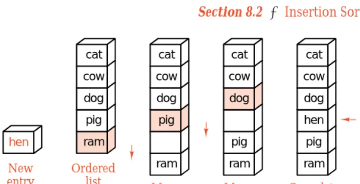
This method is illustrated in Figure 8.2, which shows the steps needed to sort example
a list of six words. At each stage, the words that have not yet been inserted into the sorted list are shown in colored boxes, and the sorted part of the list is shown in white boxes. In the initial diagram, the first wordhenis shown as sorted, since a list of length 1 is automatically ordered. All the remaining words are shown as unsorted at this stage. At each step of the process, the first unsorted word (shown in the uppermost gray box) is inserted into its proper position in the sorted part of the list. To make room for the insertion, some of the sorted words must be moved down the list. Each move of a word is shown as a colored arrow in Figure 8.2. By starting at the end of the sorted part of the list, we can move entries at the same time as we do comparisons to find where the new entry fits.
cat cow dog ewe hen ram Initial order Insert second entry Insert third entry Insert fourth entry Insert fifth entry Insert sixth entry sorted hen cow cat ram ewe dog cat cow hen ram ewe dog cat cow hen ram ewe dog cat cow ewe hen ram dog cow hen cat ram ewe dog sorted . . . . . . . sorted unsorted . . . . . .
Figure 8.2. Example of insertion sort
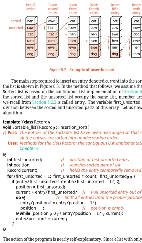
The main step required to insert an entry denotedcurrentinto the sorted part of the list is shown in Figure 8.3. In the method that follows, we assume that theclass Sorted_list is based on the contiguousListimplementation ofSection 6.2.2. Both the sorted list and the unsorted list occupy the sameList, member array, which we recall fromSection 6.2.2is calledentry. The variablefirst_unsortedmarks the division between the sorted and unsorted parts of this array. Let us now write the algorithm.
253
template<classRecord>
voidSortable_list<Record>::insertion_sort( )
/*Post: The entries of the Sortable_list have been rearranged so that the keys in all the entries are sorted into nondecreasing order.
Uses:Methods for the class Record; the contiguous List implementation of
Chapter 6*/
{
intfirst_unsorted; // position of first unsorted entry
intposition; // searches sorted part of list
Record current; // holds the entry temporarily removed from list
for(first_unsorted = 1; first_unsorted<count; first_unsorted++) if(entry[first_unsorted] <entry[first_unsorted−1]){
position = first_unsorted;
current = entry[first_unsorted]; // Pull unsorted entry out of the list.
do{ // Shift all entries until the proper position is found.
entry[position]= entry[position−1];
position−−; // position is empty.
}while(position>0&&entry[position−1] >current); entry[position]= current;
} }
The action of the program is nearly self-explanatory. Since a list with only one entry is automatically sorted, the loop onfirst_unsortedstarts with the second entry. If it is in the correct position, nothing needs to be done. Otherwise, the new entry
Section 8.2 • Insertion Sort
323
Unsorted Sorted ≤ current > current Remove current;shift entries right Before: Sorted current Unsorted Sorted Sorted Unsorted ≤ current Reinsert current; > current
Figure 8.3. The main step of contiguous insertion sort
is pulled out of the list into the variablecurrent, and thedo. . . whileloop pushes 252
entries one position down the list until the correct position is found, and finally current is inserted there before proceeding to the next unsorted entry. The case when currentbelongs in the first position of the list must be detected specially, since in this case there is no entry with a smaller key that would terminate the search. We treat this special case as the first clause in the condition of thedo. . . whileloop.
8.2.3 Linked Version
For a linked version of insertion sort, since there is no movement of data, there is no need to start searching at the endof the sorted sublist. Instead, we shall traverse the original list, taking one entry at a time and inserting it in the proper position in the sorted list. The pointer variablelast_sortedwill reference the end of the sorted part of the list, andlast_sorted->nextwill reference the first entry that algorithm
has not yet been inserted into the sorted sublist. We shall letfirst_unsortedalso point to this entry and use a pointercurrentto search the sorted part of the list to find where to insert*first_unsorted. If*first_unsortedbelongs before the current head of the list, then we insert it there. Otherwise, we move currentdown the 254
list untilfirst_unsorted->entry<=current->entryand then insert*first_unsorted before *current. To enable insertion before *current we keep a second pointer trailingin lock step one position closer to the head thancurrent.
Asentinelis an extra entry added to one end of a list to ensure that a loop will stopping the loop
terminate without having to include a separate check. Since we have last_sorted->next = first_unsorted,
the node*first_unsortedis already in position to serve as a sentinel for the search, and the loop movingcurrentis simplified.
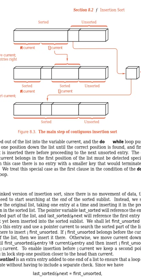
Finally, let us note that a list with 0 or 1 entry is already sorted, so that we can check these cases separately and thereby avoid trivialities elsewhere. The details appear in the following function and are illustrated in Figure 8.4.
255 template<classRecord>
voidSortable_list<Record>::insertion_sort( )
/*Post: The entries of the Sortable_list have been rearranged so that the keys in all the entries are sorted into nondecreasing order.
Uses:Methods for the class Record. The linked List implementation of
Chapter 6.*/
{
Node<Record> *first_unsorted, // the first unsorted node to be inserted *last_sorted, // tail of the sorted sublist
*current, // used to traverse the sorted sublist *trailing; // one position behind current
if(head!=NULL){ // Otherwise, the empty list is already sorted.
last_sorted = head; // The first node alone makes a sorted sublist.
while(last_sorted->next!=NULL){
first_unsorted = last_sorted->next; if(first_unsorted->entry<head->entry){
// Insert*first_unsorted at the head of the sorted list: last_sorted->next = first_unsorted->next;
first_unsorted->next = head; head = first_unsorted;
}
else{
// Search the sorted sublist to insert*first_unsorted: trailing = head;
current = trailing->next;
while(first_unsorted->entry>current->entry){
trailing = current; current = trailing->next;
}
// *first_unsorted now belongs between*trailing and*current. if(first_unsorted == current)
last_sorted = first_unsorted; // already in right position
else{
last_sorted->next = first_unsorted->next; first_unsorted->next = current;
trailing->next = first_unsorted;
} } } } }
Section 8.2 • Insertion Sort
325
last_sorted first_unsorted last_sorted Case 1: Case 2: head Partially sorted:*first_unsorted belongs at head of list
*first_unsorted belongs between *trailing and *current
head first_unsorted
head trailing current last_sorted first_unsorted
Figure 8.4. Trace of linked insertion sort
Even though the mechanics of the linked version are quite different from those of the contiguous version, you should be able to see that the basic method is the same. The only real difference is that the contiguous version searches the sorted sublist 256
in reverse order, while the linked version searches it in increasing order of position within the list.
8.2.4 Analysis
Since the basic ideas are the same, let us analyze only the performance of the contiguous version of the program. We also restrict our attention to the case when assumptions
the list is initially in random order (meaning that all possible orderings of the keys are equally likely). When we deal with entryi, how far back must we go to insert it? There areipossible ways to move it: not moving it at all, moving it one position, up to moving iti−1 positions to the front of the list. Given randomness, these are equally likely. The probability that it need not be moved is thus 1/i, in which case only one comparison of keys is done, with no moving of entries.
The remaining case, in which entryimust be moved, occurs with probability (i−1)/i. Let us begin by counting the average number of iterations of thedo. . . inserting one entry
whileloop. Since all of thei−1 possible positions are equally likely, the average number of iterations is 1+2+ · · · +(i−1) i−1 = (i−1)i 2(i−1) = i 2.
(This calculation uses Theorem A.1 on page 647.) One key comparison and one assignment are done for each of these iterations, with one more key comparison done outside the loop, along with two assignments of entries. Hence, in this second case, entryirequires, on average, 12i+1 comparisons and 12i+2 assignments.
When we combine the two cases with their respective probabilities, we have 1 i ×1+ i−1 i × i 2 +1 = i+1 2 comparisons and 1 i ×0+ i−1 i × i 2 +2 = i+3 2 − 2 i assignments.
We wish to add these numbers fromi=2 toi=n, but to avoid complications inserting all entries
in the arithmetic, we first use the big-Onotation (seeSection 7.6.3) to approximate each of these expressions by suppressing the terms bounded by a constant; that is, terms that areO(1). We thereby obtain 12i+O(1)for both the number of compar-isons and the number of assignments of entries. In making this approximation, we are really concentrating on the actions within the main loop and suppressing any concern about operations done outside the loop or variations in the algorithm that change the amount of work only by some bounded amount.
To add 12i+O(1)fromi=2 toi=n, we applyTheorem A.1 on page 647(the sum of the integers from 1 ton). We also note that addingnterms, each of which isO(1), produces as result that isO(n). We thus obtain
257 n X i=2 1 2i+O(1) = 1 2 n X i=2 i+O(n)= 1 4n2 +O(n)
for both the number of comparisons of keys and the number of assignments of entries.
So far we have nothing with which to compare this number, but we can note that as n becomes larger, the contributions from the term involving n2 become much larger than the remaining terms collected as O(n). Hence as the size of the list grows, the time needed by insertion sort grows like the square of this size.
The worst-case analysis of insertion sort will be left as an exercise. We can best and worst cases
observe quickly that the best case for contiguous insertion sort occurs when the list is already in order, when insertion sort will do nothing except n−1 comparisons of keys. We can now show that there is no sorting method that can possibly do better in its best case.
Theorem 8.1. Verifying that a list ofnentries is in the correct order requires at leastn−1 compar-isons of keys.
Section 8.2 • Insertion Sort
327
Proof Consider an arbitrary program that checks whether a list ofnentries is in order or not (and perhaps sorts it if it is not). The program will first do some comparison of keys, and this comparison will involve some two entries from the list. Sometime later, at least one of these two entries must be compared with a third, or else there would be no way to decide where these two should be in the list relative to the third. Thus this second comparison involves only one new entry not previously in a comparison. Continuing in this way, we see that there must be another comparison involving some one of the first three entries and one new entry. Note that we are not necessarily selecting the comparisons in the order in which the algorithm does them. Thus, except for the first comparison, each one that we select involves only one new entry not previously compared. All n of the entries must enter some comparison, for there is no way to decide whether an entry is in the right position unless it is compared to at least one other entry. Thus to involve all n entries requires at leastn−1 comparisons, and the proof is complete.end of proof end of proof
With this theorem we find one of the advantages of insertion sort: It verifies that a list is correctly sorted as quickly as can be done. Furthermore, insertion sort remains an excellent method whenever a list is nearly in the correct order and few entries are many positions away from their correct locations.
Exercises 8.2
E1. By hand, trace through the steps insertion sort will use on each of the following lists. In each case, count the number of comparisons that will be made and the number of times an entry will be moved.(a) The following three words to be sorted alphabetically: triangle square pentagon
(b) The three words in part (a) to be sorted according to the number of sides of the corresponding polygon, in increasing order
(c) The three words in part (a) to be sorted according to the number of sides of the corresponding polygon, in decreasing order
(d) The following seven numbers to be sorted into increasing order: 26 33 35 29 19 12 22
(e) The same seven numbers in a different initial order, again to be sorted into increasing order:
12 19 33 26 29 35 22
(f) The following list of 14 names to be sorted into alphabetical order: Tim Dot Eva Roy Tom Kim Guy Amy Jon Ann Jim Kay Ron Jan
E2. What initial order for a list of keys will produce the worst case for insertion sort in the contiguous version? In the linked version?
E3. How many key comparisons and entry assignments does contiguous insertion sort make in its worst case?
E4. Modify the linked version of insertion sort so that a list that is already sorted, or nearly so, will be processed rapidly.
Programming
Projects 8.2
P1. Write a program that can be used to test and evaluate the performance of insertion sort and, later, other methods. The following outline should be used.
(a) Create several files of integers to be used to test sorting methods. Make files of several sizes, for example, sizes 20, 200, and 2000. Make files that are in order, in reverse order, in random order, and partially in order. By test program for
sorting keeping all this test data in files (rather than generating it with random numbers each time the testing program is run), the same data can be used to test different sorting methods, and hence it will be easier to compare their performance.
(b) Write a menu-driven program for testing various sorting methods. One option is to read a file of integers into a list. Other options will be to run one of various sorting methods on the list, to print the unsorted or the sorted list, and to quit. After the list is sorted and (perhaps) printed, it should be discarded so that testing a later sorting method will start with the same input data. This can be done either by copying the unsorted list to a second list and sorting that one, or by arranging the program so that it reads the data file again before each time it starts sorting.
(c) Include code in the program to calculate and print (1) the CPU time, (2) the number of comparisons of keys, and (3) the number of assignments of list entries during sorting a list. Counting comparisons can be achieved, as inSection 7.2, by overloading the comparison operators for the classKey so that they increment a counter. In a similar way we can overload the assignment operator for the classRecordto keep a count of assignments of entries.
(d) Use the contiguous list package as developed inSection 6.2.2, include the contiguous version of insertion sort, and assemble statistics on the perfor-mance of contiguous insertion sort for later comparison with other meth-ods.
(e) Use the linked list package as developed inSection 6.2.3, include the linked version of insertion sort, assemble its performance statistics, and compare them with contiguous insertion sort. Why is the count of entry assignments of little interest for this version?
P2. Rewrite the contiguous version of the functioninsertion_sortso that it uses binary search to locate where to insert the next entry. Compare the time needed binary insertion sort
to sort a list with that of the original functioninsertion_sort. Is it reasonable to use binary search in the linked version ofinsertion_sort? Why or why not?
P3. There is an even easier sorting method, which, instead of using two pointers to move through the list, uses only one. We can call itscan sort, and it proceeds scan sort
by starting at one end and moving forward, comparing adjacent pairs of keys, until it finds a pair out of order. It then swaps this pair of entries and starts moving the other way, continuing to swap pairs until it finds a pair in the correct order. At this point it knows that it has moved the one entry as far back as necessary, so that the first part of the list is sorted, but, unlike insertion sort,
Section 8.3 • Selection Sort
329
it has forgotten how far forward has been sorted, so it simply reverses direction and sorts forward again, looking for a pair out of order. When it reaches the far end of the list, then it is finished.(a) Write a C++ program to implement scan sort for contiguous lists. Your program should use only one position variable (other than the list’scount member), one variable of typeentryto be used in making swaps, and no other local variables.
(b) Compare the timings for your program with those ofinsertion_sort.
P4. A well-known algorithm calledbubble sortproceeds by scanning the list from left to right, and whenever a pair of adjacent keys is found to be out of order, then those entries are swapped. In this first pass, the largest key in the list bubble sort
will have “bubbled” to the end, but the earlier keys may still be out of order. Thus the pass scanning for pairs out of order is put in a loop that first makes the scanning pass go all the way tocount, and at each iteration stops it one position sooner. (a) Write a C++ function for bubble sort. (b) Find the performance of bubble sort on various kinds of lists, and compare the results with those for insertion sort.
8.3 SELECTION SORT
Insertion sort has one major disadvantage. Even after most entries have been sorted properly into the first part of the list, the insertion of a later entry may require that many of them be moved. All the moves made by insertion sort are moves of only one position at a time. Thus to move an entry 20 positions up the list requires 20 separate moves. If the entries are small, perhaps a key alone, or if the entries are in linked storage, then the many moves may not require excessive time. But if the entries are very large, records containing hundreds of components like personnel files or student transcripts, and the records must be kept in contiguous storage, then it would be far more efficient if, when it is necessary to move an entry, it could be moved immediately to its final position. Our next sorting method accomplishes this goal.
8.3.1 The Algorithm
An example of this sorting method appears in Figure 8.5, which shows the steps needed to sort a list of six words alphabetically. At the first stage, we scan the list to find the word that comes last in alphabetical order. This word,ram, is shown in a colored box. We then exchange this word with the word in the last position, as shown in the second part of Figure 8.5. Now we repeat the process on the shorter list obtained by omitting the last entry. Again the word that comes last is shown in a colored box; it is exchanged with the last entry still under consideration; and so we continue. The words that are not yet sorted into order are shown in gray boxes at each stage, except for the one that comes last, which is shown in a colored box. When the unsorted list is reduced to length 1, the process terminates.
258 Initial order
Colored box denotes largest unsorted key. Gray boxes denote other unsorted keys.
Sorted hen cow cat dog ewe ram ewe cow cat dog hen ram dog cow cat ewe hen ram cat cow dog ewe hen ram cat cow dog ewe hen ram hen cow cat ram ewe dog
Figure 8.5. Example of selection sort
This method translates into an algorithm called selection sort. The general step in selection sort is illustrated in Figure 8.6. The entries with large keys will be sorted in order and placed at the end of the list. The entries with smaller keys are not yet sorted. We then look through the unsorted entries to find the one with the largest key and swap it with the last unsorted entry. In this way, at each pass through the main loop, one more entry is placed in its final position.
Unsorted small keys Sorted, large keys Maximum unsorted key Swap Current position
Unsorted small keys Sorted, large keys
Figure 8.6. The general step in selection sort
8.3.2 Contiguous Implementation
Since selection sort minimizes data movement by putting at least one entry in its final position at every pass, the algorithm is primarily useful for contiguous lists with large entries for which movement of entries is expensive. If the entries are small, or if the list is linked, so that only pointers need be changed to sort the list, then insertion sort is usually faster than selection sort. We therefore give only a contiguous version of selection sort. The algorithm uses an auxiliarySortable_list member function calledmax_key, which finds the maximum key on a part of the list that is specified by parameters. The auxiliary functionswapsimply swaps the two entries with the given indices. For convenience in the discussion to follow, we write these two as separate auxiliary member functions:
Section 8.3 • Selection Sort
331
259template<classRecord>
voidSortable_list<Record>::selection_sort( )
/*Post: The entries of the Sortable_list have been rearranged so that the keys in all the entries are sorted into nondecreasing order.
Uses:max_key, swap.*/
{
for(intposition = count−1; position>0; position−−){ intmax = max_key(0,position);
swap(max,position);
} }
Note that when all entries but one are in the correct position in a list, then the remaining one must be also. Thus theforloop stops at 1.
template<classRecord>
intSortable_list<Record>::max_key(intlow, inthigh)
/*Pre: low and high are valid positions in the Sortable_list and low<=high. Post: The position of the entry between low and high with the largest key is
returned.
Uses:The class Record. The contiguous List implementation ofChapter 6.*/
{
intlargest,current; largest = low;
for(current = low+1; current<=high; current++) if(entry[largest] <entry[current])
largest = current; returnlargest;
}
260
template<classRecord>
voidSortable_list<Record>::swap(intlow, inthigh)
/*Pre: low and high are valid positions in the Sortable_list.
Post: The entry at position low is swapped with the entry at position high.
Uses:The contiguous List implementation ofChapter 6.*/
{
Record temp; temp = entry[low]; entry[low]= entry[high]; entry[high]= temp;
}
8.3.3 Analysis
À propos of algorithm analysis, the most remarkable fact about this algorithm is that both of the loops that appear areforloops with completely predictable ranges, which means that we can calculate in advance exactly how many times they will iterate. In the number of comparisons it makes, selection sort pays no attention to
the original ordering of the list. Hence for a list that is in nearly correct order to ordering unimportant
begin with, selection sort is likely to be much slower than insertion sort. On the other hand, selection sort does have the advantage of predictability: Its worst-case time will differ little from its best.
The primary advantage of selection sort regards data movement. If an entry advantage of
selection sort is in its correct final position, then it will never be moved. Every time any pair of entries is swapped, then at least one of them moves into its final position, and therefore at mostn−1 swaps are done altogether in sorting a list ofnentries. This is the very best that we can expect from any method that relies entirely on swaps to move its entries.
We can analyze the performance of functionselection_sortin the same way analysis
that it is programmed. The main function does nothing except some bookkeeping and calling the subprograms. The functionswapis calledn−1 times, and each call does 3 assignments of entries, for a total count of 3(n−1). The functionmax_key is calledn−1 times, with the length of the sublist ranging fromndown to 2. Iftis the number of entries on the part of the list for which it is called, thenmax_keydoes exactlyt−1 comparisons of keys to determine the maximum. Hence, altogether, comparison count for
selection sort there are (n−1)+(n−2)+ · · · +1 = 1
2n(n−1)comparisons of keys, which we approximate to 12n2+O(n).
8.3.4 Comparisons
Let us pause for a moment to compare the counts for selection sort with those for insertion sort. The results are:
260
Selection Insertion (average) Assignments of entries 3.0n+O(1) 0.25n2+O(n) Comparisons of keys 0.5n2+O(n) 0.25n2+O(n)
The relative advantages of the two methods appear in these numbers. When n becomes large, 0.25n2 becomes much larger than 3n, and if moving entries is a slow process, then insertion sort will take far longer than will selection sort. But the amount of time taken for comparisons is, on average, only about half as much for insertion sort as for selection sort. If the list entries are small, so that moving them is not slow, then insertion sort will be faster than selection sort.
Exercises 8.3
E1. By hand, trace through the steps selection sort will use on each of the following lists. In each case, count the number of comparisons that will be made and the number of times an entry will be moved.(a) The following three words to be sorted alphabetically: triangle square pentagon
(b) The three words in part (a) to be sorted according to the number of sides of the corresponding polygon, in increasing order
Section 8.4 • Shell Sort
333
(c) The three words in part (a) to be sorted according to the number of sides of the corresponding polygon, in decreasing order
(d) The following seven numbers to be sorted into increasing order: 26 33 35 29 19 12 22
(e) The same seven numbers in a different initial order, again to be sorted into increasing order:
12 19 33 26 29 35 22
(f) The following list of 14 names to be sorted into alphabetical order: Tim Dot Eva Roy Tom Kim Guy Amy Jon Ann Jim Kay Ron Jan
E2. There is a simple algorithm calledcount sortthat begins with an unsorted list and constructs a new, sorted list in a new array, provided we are guaranteed count sort
that all the keys in the original list are different from each other. Count sort goes through the list once, and for each record scans the list to count how many records have smaller keys. If c is this count, then the proper position in the sorted list for this key isc. Determine how many comparisons of keys will be done by count sort. Is it a better algorithm than selection sort?
Programming
Projects 8.3
P1. Run the test program written inProject P1 of Section 8.2 (page 328), to compare selection sort with insertion sort (contiguous version). Use the same files of test data used with insertion sort.
P2. Write and test a linked version of selection sort.
8.4 SHELL SORT
As we have seen, in some ways insertion sort and selection sort behave in opposite ways. Selection sort moves the entries very efficiently but does many redundant comparisons. In its best case, insertion sort does the minimum number of compar-isons, but it is inefficient in moving entries only one position at a time. Our goal now is to derive another method that avoids, as much as possible, the problems with both of these. Let us start with insertion sort and ask how we can reduce the number of times it moves an entry.
The reason why insertion sort can move entries only one position is that it compares only adjacent keys. If we were to modify it so that it first compares keys far apart, then it could sort the entries far apart. Afterward, the entries closer together would be sorted, and finally the increment between keys being compared would be reduced to 1, to ensure that the list is completely in order. This is the idea implemented in 1959 by D. L. SHELLin the sorting method bearing his name. This method is also sometimes calleddiminishing-increment sort. Before describing diminishing
increments the algorithm formally, let us work through a simple example of sorting names. example Figure 8.7 shows what will happen when we first sort all names that are at
distance 5 from each other (so there will be only two or three names on each such list), then re-sort the names using increment 3, and finally perform an ordinary insertion sort (increment 1).
Unsorted Tim Dot Eva Roy Tom Kim Guy Amy Jon Ann Jim Kay Ron Jan Sublists incr. 5
Sublists incr. 3 3-Sorted
Dot Eva Tim Roy Tom Recombined Jim Dot Amy Jan Ann Kim Guy Eva Jon Tom Tim Kay Ron Roy List incr. 1 Guy Ann Amy Jan Dot Jon Jim Eva Kay Ron Roy Kim Tom Tim Sorted Amy Ann Dot Eva Guy Jan Jim Jon Kay Kim Ron Roy Tim Tom 5-Sorted Dot Amy Jim Jan Ann Guy Amy Kim Jon Ann Kay Ron Jim Jan Guy Eva Kim Jon Tom Kay Ron Tim Roy Jim Dot Amy Jan Ann Kim Guy Eva Jon Tom Tim Kay Ron Roy Guy Ann Amy Jan Dot Jon Jim Eva Kay Ron Roy Kim Tom Tim
Figure 8.7. Example of Shell sort
You can see that, even though we make three passes through all the names, the 261 early passes move the names close to their final positions, so that at the final pass (which does an ordinary insertion sort), all the entries are very close to their final positions so the sort goes rapidly.
choice of increments There is no magic about the choice of 5, 3, and 1 as increments. Many other choices might work as well or better. It would, however, probably be wasteful to choose powers of 2, such as 8, 4, 2, and 1, since then the same keys compared on one pass would be compared again at the next, whereas by choosing numbers that are not multiples of each other, there is a better chance of obtaining new information from more of the comparisons. Although several studies have been made of Shell sort, no one has been able to prove that one choice of the increments is greatly superior to all others. Various suggestions have been made. If the increments are chosen close together, as we have done, then it will be necessary to make more passes, but each one will likely be quicker. If the increments decrease rapidly, then fewer but longer passes will occur. The only essential feature is that the final increment be 1, so that at the conclusion of the process, the list will be checked to be completely in order. For simplicity in the following algorithm, we start with increment == count, where we recall fromSection 6.2.2thatcountrepresents the size of theListbeing sorted, and at each pass reduce the increment with a statement
Section 8.4 • Shell Sort
335
Thus the increments used in the algorithm are not the same as those used in Figure 8.7.We can now outline the algorithm for contiguous lists. 262
template<classRecord>
voidSortable_list<Record>::shell_sort( )
/*Post: The entries of the Sortable_list have been rearranged so that the keys in all the entries are sorted into nondecreasing order.
Uses:sort_interval*/
{
intincrement, // spacing of entries in sublist
start; // starting point of sublist
increment = count; do{
increment = increment/3+1;
for(start = 0; start<increment; start++)
sort_interval(start,increment); // modified insertion sort }while(increment>1);
}
The auxiliary member functionsort_interval(intstart, intincrement)is exactly the functioninsertion_sort, except that the list starts at the variablestartinstead of 0 and the increment between successive values is as given instead of 1. The details of modifyinginsertion_sortintosort_intervalare left as an exercise.
Since the final pass through Shell sort has increment 1, Shell sort really is insertion sort optimized by the preprocessing stage of first sorting sublists using optimized insertion
sort larger increments. Hence the proof that Shell sort works correctly is exactly the same as the proof that insertion sort works correctly. And, although we have good reason to think that the preprocessing stage will speed up the sorting considerably by eliminating many moves of entries by only one position, we have not actually proved that Shell sort will ever be faster than insertion sort.
analysis The analysis of Shell sort turns out to be exceedingly difficult, and to date, good estimates on the number of comparisons and moves have been obtained only under special conditions. It would be very interesting to know how these numbers depend on the choice of increments, so that the best choice might be made. But even without a complete mathematical analysis, running a few large examples on a computer will convince you that Shell sort is quite good. Very large empirical studies have been made of Shell sort, and it appears that the number of moves, when nis large, is in the range of n1.25to 1.6n1.25. This constitutes a substantial improvement over insertion sort.
Exercises 8.4
E1. By hand, sort the list of 14 names in the “unsorted” column ofFigure 8.7using Shell sort with increments of (a) 8, 4, 2, 1 and (b) 7, 3, 1. Count the number of comparisons and moves that are made in each case.Programming
Projects 8.4
P1. Rewrite the methodinsertion_sortto serve as the functionsort_interval em-bedded inshell_sort.
P2. Testshell_sortwith the program ofProject P1 of Section 8.2 (page 328), using the same data files as for insertion sort, and compare the results.
8.5 LOWER BOUNDS
Now that we have seen a method that performs much better than our first attempts, it is appropriate to ask,
263
How fast is it possible to sort?
To answer, we shall limit our attention (as we did when answering the same ques-tion for searching) to sorting methods that rely entirely on comparisons between pairs of keys to do the sorting.
Let us take an arbitrary sorting algorithm of this class and consider how it sorts a list ofnentries. Imagine drawing its comparison tree. Sample comparison trees comparison tree
for insertion sort and selection sort applied to three numbersa,b,c are shown in Figure 8.8. As each comparison of keys is made, it corresponds to an interior vertex (drawn as a circle). The leaves (square nodes) show the order that the numbers have after sorting.
Insertion sort Selection sort F F F T T T a ≤ b b ≤ c a ≤ b ≤ c a ≤ c b < a ≤ c c < b < a c < a ≤ b a ≤ c < b a < b a < c b < c c < b a < b a < c b ≤ c ≤ a c < b ≤ a b ≤ c < a b ≤ a < c impossible c ≤ a < b a < c ≤ b impossible a < b < c F T F T F T F T a < b F F F T T T F T F T a ≤ c b ≤ c
Section 8.5 • Lower Bounds
337
Note that the diagrams show clearly that, on average, selection sort makes more comparisons of keys than insertion sort. In fact, selection sort makes redundant comparisons, repeating comparisons that have already been made.The comparison tree of an arbitrary sorting algorithm displays several features of the algorithm. Its height is the largest number of comparisons that will be made comparison trees:
height and path length and hence gives the worst-case behavior of the algorithm. The external path length, after division by the number of leaves, gives the average number of comparisons that the algorithm will do. The comparison tree displays all the possible sequences of comparisons that can be made as all the different paths from the root to the leaves. Since these comparisons control how the entries are rearranged during sorting, any two different orderings of the list must result in some different decisions, and hence different paths through the tree, which must then end in different leaves. The number of ways that the list containingnentries could originally have been ordered isn! (seeSection A.3.1), and thus the number of leaves in the tree must be at leastn!. Lemma 7.5now implies that the height of the tree is at leastdlgn!eand its external path length is at leastn! lgn!. (Recall thatdkemeans the smallest integer not less thank.) Translating these results into the number of comparisons, we obtain Theorem 8.2 Any algorithm that sorts a list ofn entries by use of key comparisons must, in its
worst case, perform at leastdlgn!ecomparisons of keys, and, in the average case, it must perform at leastlgn!comparisons of keys.
Stirling’s formula (Theorem A.5 on page 658) gives an approximation to the factorial of an integer, which, after taking the base 2 logarithm, is
lgn! ≈ (n+ 1
2)lgn−(lge)n+lg p
2π + lge
12n. The constants in this expression have the approximate values approximating lgn!
lge ≈ 1.442695041 and lgp2π ≈ 1.325748069.
Stirling’s approximation to lgn! is very close indeed, much closer than we shall ever need for analyzing algorithms. For almost all purposes, the following rough approximation will prove quite satisfactory:
lgn! ≈ (n+ 1
2)(lgn−112)+2
and often we use only the approximation lgn!=nlgn+O(n).
Before ending this section we should note that there are sometimes methods for sorting that do not use comparisons and can be faster. For example, if you know other methods
in advance that you have 100 entries and that their keys are exactly the integers between 1 and 100 in some order, with no duplicates, then the best way to sort them is not to do any comparisons, but simply, if a particular entry has keyi, then place it in locationi. With this method we are (at least temporarily) regarding the entries to be sorted as being in a table rather than a list, and then we can use the key as an index to find the proper position in the table for each entry. Project P1 suggests an extension of this idea to an algorithm.
Exercises 8.5
E1. Draw the comparison trees for (a) insertion sort and (b) selection sort applied to four objects.E2. (a)Find a sorting method for four keys that is optimal in the sense of doing the smallest possible number of key comparisons in its worst case. (b) Find how many comparisons your algorithm does in the average case (applied to four keys). Modify your algorithm to make it come as close as possible to achieving the lower bound of lg 4! ≈ 4.585 key comparisons. Why is it impossible to achieve this lower bound?
E3. Suppose that you have a shuffled deck of 52 cards, 13 cards in each of 4 suits, and you wish to sort the deck so that the 4 suits are in order and the 13 cards within each suit are also in order. Which of the following methods is fastest?
(a) Go through the deck and remove all the clubs; then sort them separately. Proceed to do the same for the diamonds, the hearts, and the spades.
(b) Deal the cards into 13 piles according to the rank of the card. Stack these 13 piles back together and deal into 4 piles according to suit. Stack these back together.
(c) Make only one pass through the cards, by placing each card in its proper position relative to the previously sorted cards.
Programming
Projects 8.5
The sorting projects for this section are specialized methods requiring keys of a particular type, pseudorandom numbers between 0 and 1. Hence they are not intended to work with the testing program devised for other methods, nor to use the same data as the other methods studied in this chapter.
P1. Construct a list ofnpseudorandom numbers strictly between 0 and 1. Suitable values for n are 10 (for debugging) and 500 (for comparing the results with other methods). Write a program to sort these numbers into an array via the followinginterpolation sort. First, clear the array (to all 0). For each number interpolation sort
from the old list, multiply it byn, take the integer part, and look in that position of the table. If that position is 0, put the number there. If not, move left or right (according to the relative size of the current number and the one in its place) to find the position to insert the new number, moving the entries in the table over if necessary to make room (as in the fashion of insertion sort). Show that your algorithm will really sort the numbers correctly. Compare its running time with that of the other sorting methods applied to randomly ordered lists of the same size.
P2. [suggested by B. LEE] Write a program to perform a linked distribution sort, as follows. Take the keys to be pseudorandom numbers between 0 and 1, as in the previous project. Set up an array of linked lists, and distribute the keys linked distribution
sort into the linked lists according to their magnitude. The linked lists can either be kept sorted as the numbers are inserted or sorted during a second pass, during which the lists are all connected together into one sorted list. Experiment to determine the optimum number of lists to use. (It seems that it works well to have enough lists so that the average length of each list is about 3.)
Section 8.6 • Divide-and-Conquer Sorting
339
8.6 DIVIDE-AND-CONQUER SORTING
8.6.1 The Main Ideas
Making a fresh start is often a good idea, and we shall do so by forgetting (tem-porarily) almost everything that we know about sorting. Let us try to apply only one important principle that has shown up in the algorithms we have previously studied and that we already know from common experience: It is much easier to shorter is easier
sort short lists than long ones. If the number of entries to be sorted doubles, then the work more than doubles (with insertion or selection sort it quadruples, roughly). Hence if we can find a way to divide the list into two roughly equal-sized lists and sort them separately, then we will save work. If, for example, you were working in a library and were given a thousand index cards to put in alphabetical order, then a good way would be to distribute them into piles according to the first letter and sort the piles separately.
Here again we have an application of the idea of dividing a problem into smaller divide and conquer
but similar subproblems; that is, ofdivide and conquer.
First, we note that comparisons by computer are usually two-way branches, so we shall divide the entries to sort into two lists at each stage of the process.
What method, you may ask, should we use to sort the reduced lists? Since we have (temporarily) forgotten all the other methods we know, let us simply use the same method, divide and conquer, again, repeatedly subdividing the list. But we won’t keep going forever: Sorting a list with only one entry doesn’t take any work, even if we know no formal sorting methods.
In summary, let us informally outline divide-and-conquer sorting: 264
voidSortable_list::sort( )
{
ifthe list has length greater than 1{
partition the list into lowlist,highlist; lowlist.sort( );
highlist.sort( );
combine(lowlist,highlist);
} }
We still must decide how we are going to partition the list into two sublists and, after they are sorted, how we are going to combine the sublists into a single list. There are two methods, each of which works very well in different circumstances.
➥
Mergesort: In the first method, we simply chop the list into two sublists of sizes as nearly equal as possible and then sort them separately. Afterward, we carefully merge the two sorted sublists into a single sorted list. Hence this mergesortmethod is calledmergesort.
➥
Quicksort: The second method does more work in the first step of partition-ing the list into two sublists, and the final step of combinpartition-ing the sublists then becomes trivial. This method was invented and christened quicksort quicksortby C. A. R. HOARE. To partition the list, we first choose some key from the list for which, we hope, about half the keys will come before and half after. We shall use the namepivotfor this selected key. We next partition the entries so pivot
that all those with keys less than the pivot come in one sublist, and all those with greater keys come in another. Finally, then, we sort the two reduced lists separately, put the sublists together, and the whole list will be in order.
8.6.2 An Example
Before we refine our methods into detailed functions, let us work through a specific example. We take the following seven numbers to sort:
26 33 35 29 19 12 22.
1. Mergesort Example
The first step of mergesort is to chop the list into two. When (as in this example) convention: left list
may be longer the list has odd length, let us establish the convention of making the left sublist one entry larger than the right sublist. Thus we divide the list into
26 33 35 29 and 19 12 22
and first consider the left sublist. It is again chopped in half as first half
26 33 and 35 29.
For each of these sublists, we again apply the same method, chopping each of them into sublists of one number each. Sublists of length one, of course, require no sorting. Finally, then, we can start to merge the sublists to obtain a sorted list. The sublists 26 and 33 merge to give the sorted list 26 33, and the sublists 35 and 29 merge to give 29 35. At the next step, we merge these two sorted sublists of length two to obtain a sorted sublist of length four,
26 29 33 35.
Now that the left half of the original list is sorted, we do the same steps on the right half. First, we chop it into the sublists
second half
19 12 and 22.
The first of these is divided into two sublists of length one, which are merged to give 12 19. The second sublist, 22, has length one, so it needs no sorting. It is now merged with 12 19 to give the sorted list
12 19 22.
Finally, the sorted sublists of lengths four and three are merged to produce 12 19 22 26 29 33 35.
The way that all these sublists and recursive calls are put together is shown by the recursion tree for mergesort drawn in Figure 8.9. The order in which the recursive calls occur is shown by the colored path. The numbers in each sublist passed to a recursive call are shown in black, and the numbers in their order after the merge is done are shown in color. The calls for which no further recursion is required (sublists of length 1) are the leaves of the tree and are drawn as squares.
Section 8.6 • Divide-and-Conquer Sorting
341
265 Start Finish 26 33 35 29 19 12 26 33 26 33 35 29 29 35 19 12 12 19 26 33 35 29 26 29 33 35 19 12 22 12 19 22 22 29 19 12 22 35 33 26 12 19 22 26 29 33 35Figure 8.9. Recursion tree, mergesort of 7 numbers
2. Quicksort Example
Let us again work through the same example, this time applying quicksort and keeping careful account of the execution of steps from our outline of the method. To use quicksort, we must first decide, in order to partition the list into two pieces, choice of pivot
what key to choose as the pivot. We are free to choose any number we wish, but, for consistency, we shall adopt a definite rule. Perhaps the simplest rule is to choose the first number in a list as the pivot, and we shall do so in this example. For practical applications, however, other choices are usually better than the first number.
Our first pivot, then, is 26, and the list partitions into sublists partition
19 12 22 and 33 35 29
consisting, respectively, of the numbers less than and greater than the pivot. We have left the order of the entries in the sublists unchanged from that in the original list, but this decision also is arbitrary. Some versions of quicksort put the pivot into one of the sublists, but we choose to place the pivot into neither sublist.
We now arrive at the next line of the outline, which tells us to sort the first sublist. We thus start the algorithm over again from the top, but this time applied to the shorter list
19 12 22.
The pivot of this list is 19, which partitions its list into two sublists of one number lower half
each, 12 in the first and 22 in the second. With only one entry each, these sublists do not need sorting, so we arrive at the last line of the outline, whereupon we combine the two sublists with the pivot between them to obtain the sorted list
12 19 22.
Now the call to the sort function is finished for this sublist, so it returns whence it was called. It was called from within the sort function for the full list of seven numbers, so we now go on to the next line of that function.
inner and outer function calls
We have now used the function twice, with the second instance occurring within the first instance. Note carefully that the two instances of the function are working on different lists and are as different from each other as is executing the same code twice within a loop. It may help to think of the two instances as having different colors, so that the instructions in the second (inner) call could be written out in full in place of the call, but in a different color, thereby clearly distinguishing them as a separate instance of the function. The steps of this process are illustrated in Figure 8.10.
266
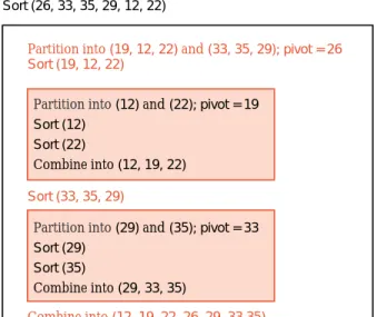
Sort (26, 33, 35, 29, 12, 22)
Partition into (19, 12, 22) and (33, 35, 29); pivot = 26 Sort (19, 12, 22)
Sort (33, 35, 29)
Combine into (12, 19, 22, 26, 29, 33 35) Partition into (12) and (22); pivot = 19 Sort (12)
Sort (22)
Combine into (12, 19, 22)
Partition into (29) and (35); pivot = 33 Sort (29)
Sort (35)
Combine into (29, 33, 35)
Figure 8.10. Execution trace of quicksort
Returning to our example, we find the next line of the first instance of the function to be another call to sort another list, this time the three numbers
33 35 29.
As in the previous (inner) call, the pivot 33 immediately partitions the list, giving upper half
sublists of length one that are then combined to produce the sorted list 29 33 35.
Finally, this call to sort returns, and we reach the last line of the (outer) instance that sorts the full list. At this point, the two sorted sublists of length three are combined with the original pivot of 26 to obtain the sorted list
12 19 22 26 29 33 35. After this step, the process is complete.
Section 8.6 • Divide-and-Conquer Sorting
343
The easy way to keep track of all the calls in our quicksort example is to draw its recursion tree, as shown in Figure 8.11. The two calls tosortat each level are shown as the children of the vertex. The sublists of size 1 or 0, which need no sorting, are drawn as the leaves. In the other vertices (to avoid cluttering the diagram), we include only the pivot that is used for the call. It is, however, not hard to read all the numbers in each sublist (but not necessarily in their original order). The numbers in the sublist at each recursive call are the number at the corresponding vertex and those at all descendents of the vertex.26
19 33
12 22 29 35
Figure 8.11. Recursion tree, quicksort of 7 numbers
If you are still uneasy about the workings of recursion, then you will find example
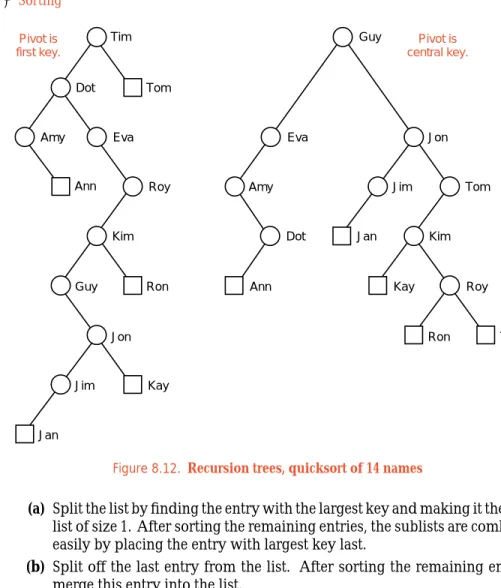
it helpful to pause and work through sorting the list of 14 names introduced in previous sections, using both mergesort and quicksort. As a check, Figure 8.12 provides the tree of calls for quicksort in the same abbreviated form used for the previous example. This tree is given for two versions, one where the pivot is the first key in each sublist, and one where the central key (center left for even-sized lists) is the pivot.
Exercises 8.6
E1. Apply quicksort to the list of seven numbers considered in this section, where the pivot in each sublist is chosen to be (a) the last number in the sublist and(b)the center (or left-center) number in the sublist. In each case, draw the tree of recursive calls.
E2. Apply mergesort to the list of 14 names considered for previous sorting meth-ods:
Tim Dot Eva Roy Tom Kim Guy Amy Jon Ann Jim Kay Ron Jan
E3. Apply quicksort to this list of 14 names, and thereby sort them by hand into alphabetical order. Take the pivot to be (a) the first key in each sublist and
(b)the center (or left-center) key in each sublist. See Figure 8.12.
E4. In both divide-and-conquer methods, we have attempted to divide the list into two sublists of approximately equal size, but the basic outline of sorting by divide-and-conquer remains valid without equal-sized halves. Consider dividing the list so that one sublist has size 1. This leads to two methods, depending on whether the work is done in splitting one element from the list or in combining the sublists.
Tim Tom Dot Amy Eva Ann Roy Kim Guy Ron Jon Jim Kay Jan Tim Tom Dot Amy Eva Ann Roy Kim Guy Ron Jon Jim Kay Jan Pivot is central key. Pivot is first key.
Figure 8.12. Recursion trees, quicksort of 14 names
(a) Split the list by finding the entry with the largest key and making it the sub-list of size 1. After sorting the remaining entries, the subsub-lists are combined easily by placing the entry with largest key last.
(b) Split off the last entry from the list. After sorting the remaining entries, merge this entry into the list.
Show that one of these methods is exactly the same method as insertion sort and the other is the same as selection sort.
8.7 MERGESORT FOR LINKED LISTS
Let us now turn to the writing of formal functions for each of our divide-and-267
conquer sorting methods. In the case of mergesort, we shall write a version for linked lists and leave the case of contiguous lists as an exercise. For quicksort, we shall do the reverse, writing the code only for contiguous lists. Both of these methods, however, work well for both contiguous and linked lists.
Mergesort is also an excellent method forexternal sorting; that is, for problems in which the data are kept on disks, not in high-speed memory.
Section 8.7 • Mergesort for Linked Lists
345
8.7.1 The Functions
When we sort a linked list, we work by rearranging the links of the list and we avoid the creation and deletion of new nodes. In particular, our mergesort pro-gram must call a recursive function that works with subsets of nodes of the list being sorted. We call this recursive functionrecursive_merge_sort. Our primary 268
implementation of mergesort simply passes a pointer to the first node of the list in a call torecursive_merge_sort.
main function template<classRecord>
voidSortable_list<Record>::merge_sort( )
/*Post: The entries of the sortable list have been rearranged so that their keys are sorted into nondecreasing order.
Uses:The linked List implementation ofChapter 6and recursive_merge_sort.*/
{
recursive_merge_sort(head);
}
Our outline of the basic method for mergesort translates directly into the following recursive sorting function.
template<classRecord>
voidSortable_list<Record>::recursive_merge_sort(Node<Record> * &sub_list) /*Post: The nodes referenced by sub_list have been rearranged so that their keys
are sorted into nondecreasing order. The pointer parameter sub_list is reset to point at the node containing the smallest key.
Uses:The linked List implementation ofChapter 6; the functions divide_from,
merge, and recursive_merge_sort.*/
{
if(sub_list!=NULL&&sub_list->next!=NULL){
Node<Record> *second_half = divide_from(sub_list); recursive_merge_sort(sub_list);
recursive_merge_sort(second_half); sub_list = merge(sub_list,second_half);
} }
Observe that the parametersub_listin the functionrecursive_merge_sortis a refer-ence to a pointer to a node. The referrefer-ence is needed to allow the function to make a change to the calling argument.
The first subsidiary function called byrecursive_merge_sort, divide_from(Node<Record> *sub_list)
takes the list referenced by the parametersub_listand divides it in half, by replacing its middle link by aNULLpointer. The function returns a pointer to the first node 269