The Labor Market Effects of Welfare Reform

The Labor Market Effects of Welfare Reform

Darren Lubotsky

Department of Economics

549 Evans Hall

University of California

Berkeley, California 94720

lubotsky@econ.berkeley.edu

April 6, 1999

The recent reform of the federal welfare system is meant to encourage recipients to leave welfare and enter the workforce. If the reform is successful there are likely to be effects felt throughout the low–skilled end of the labor market. As former welfare recipients enter the labor market, they may exert downward pressure on wages or displace employment of others already in the labor market. Since there has been limited changes in eligibility for federal welfare programs from which to draw inferences, the magnitude of these labor market effects are open to debate.

This study considers these issues in general and evaluates how labor markets in Michigan were affected when the General Assistance program in that state was elimi-nated in 1991. General Assistance was a large–scale, state–administered program that provided benefits to people who fell through the cracks in federal anti–poverty pro-grams. In all, about eighty to one–hundred thousand able–bodied adults lost benefits. Increased labor force participation among these people resulted in a decline in weekly hours among high school drop–outs of 1.2 to 2.4 percent. There is little evidence of declines in hourly earnings, except in the Detroit area, where wages fell by about five percent.

JEL Classification: H53, I3, J2.

∗_{Ph.D. candidate. I owe a special thanks to David Card for insightful advice and encouragement. I} also thank Alan Auerbach, Hilary Hoynes, Warren Hrung, Jonathan Leonard, Daniel McFadden, Jonathan Siegel, Miguel Urquiola, and participants in the UC Berkeley Public Finance Seminar and the Labor Lunch for their comments; and Jared Bernstein and David Webster of the Economic Policy Institute for providing me with the CPS monthly interview data.

1

Introduction

The 1996 reform of the federal welfare system was aimed at encouraging recipients to leave welfare and enter the workforce. To accomplish this goal, time–limitations have been placed on individuals’ receipt of benefits, and state governments are required to meet federal targets for moving welfare recipients into the workforce. State governments have also been given increased flexibility in the design and implementation of programs in order to meet these goals. If the reform is successful there are likely to be general equilibrium effects felt throughout the low–skilled end of the labor market: an increase in labor supply among former recipients would lead to downward pressure on wages or displace employment of others in the labor market. Because there have not been large changes in eligibility for benefits or in the incentives facing welfare recipients in the past, the magnitude of these effects is open to debate. Analyses of closely related changes in the labor market and welfare programs are necessary to better inform the current debate.

This study considers these issues in general and evaluates how labor markets in Michigan were affected when the General Assistance program in that state was eliminated in October, 1991. Cash benefits for able–bodied adults without children were terminated, leaving about 100,000 people – equal to about two percent of the state labor force – to turn to the labor market, their families, or other private sources for income. To identify the effect of the increase in labor force participation by former GA recipients, changes in wages, employment, labor force participation, and hours of work in Michigan are compared with changes in other states that did not reform their General Assistance program in the two years after the reform. Eleven control states from the Midwest and northeastern United States are used: New Hampshire, Massachusetts, New York, New Jersey, Pennsylvania, Ohio, Indiana, Wisconsin, Missouri, Virginia, and West Virginia.1 Given the geographic proximity and economic links between Michigan and these states, they provide a credible counterfactual of how labor markets in Michigan would have evolved in the absence of welfare reform.

A potential problem for future work on the labor market effects of federal welfare reform is

1_{In 1991 benefit levels in Ohio were reduced by about one–third, and most recipients were limited to}

receiving benefits six months out of a year. In 1992 New York set lower benefit levels for new residents in the state.

that participants nationwide were affected by the 1996 legislation. Though individual states are given vastly increased autonomy in the design of welfare programs, inter–state variation in the fall in welfare caseloads will be the result of differences in economic conditions, in state policies, and other aspects of labor markets in each state. It may be difficult, therefore, to identify the causal role of welfare reform on labor market outcomes.2 A unique feature of this evaluation is a clear counterfactual group. Much attention will be paid, however, to controlling for differences between the labor market in Michigan and in the control states that are not due to the elimination of the General Assistance program.

Of the one hundred thousand GA recipients at the time the program was eliminated, some were able to enroll in other government programs, in particular people with disabilities or with dependent children. Of the eighty–two thousand people who it is estimated lost all public transfers, if forty to fifty thousand people (roughly fifty to sixty percent) entered the labor market, that would represent an increase of 1% to 1.25% in the state labor force. More relevant, it would represent an increase of 8% to 10% of the five hundred thousand people in the state without a high school degree who were in the labor force. Because the effects of increased labor force participation among former recipients are likely to be felt most strongly in the low–skilled labor market, this analysis focuses on identifying changes in economic outcomes among people without a high school degree.

Before the estimation of econometric models, a simple theoretical model is presented that illustrates some of the important effects that welfare reform in a local economy could have on the employment and earnings of others in the labor market. This serves to highlight the relevant elasticities, as well as how the results depend on the distribution of skills throughout the locality. With earnings data from Michigan in 1990, the model is calibrated and the change in earnings and hours of workers without a high school degree are simulated. It is argued that for reasonable parameter choices, earnings are likely to decline by no more than two to four percent, and hourly of work by no more than one percent. The actual effects may be even smaller, however, based on alternative parameter choices.

The data used in this study come from the 1989 through 1993 monthly Current Population

2_{In addition, it may be some time before adequate data exists to fully assess how federal welfare reform}

Survey. The basic econometric specification is a quasi–experimental, treatment– and control– group model in which the change in individual measures of employment, hours, earnings, and labor force participation for people in Michigan before and after the elimination of the GA program are compared to the change in outcomes for people in the control states over the same time period. The model also accounts for demographic characteristics, such as age, education, and race, that are correlated with economic outcomes.

If there were differences other than the elimination of the GA program that affected labor markets in Michigan and the control states, this estimate alone does not identify the effect of the elimination of GA benefits. Therefore, an important additional feature of the identi-fication method is that differences in economic outcomes between Michigan and the control states are estimated conditional on differences between the states in business cycle effects and other unobservable labor demand shocks. Differences in labor demand are accounted for by allowing demand shocks to differentially effect the labor market outcomes of people of different ages, genders, and levels of education. These added controls are particularly important since the unemployment rate in Michigan fell considerably faster than that in the control states following the recession in the early 1990’s. This likely is a signal of different economic conditions in Michigan, other than the reform of the state welfare system there, and consequently a comparison of economic outcomes that ignores these differences will lead to a biased estimate of the effect of the elimination of the GA program.

The results show that employment among people without a high school degree – those who are most likely to be affected by increased labor market participation among former welfare recipients – increased by one to two and a half percentage points, relative to the change in employment of people with a high school degree. Average hours of work among workers fell by 1.2 to 2.4 percent. There is little evidence of declines in hourly earnings, except in the Detroit area, where wages fell by about five percent.

2

The General Assistance Program in Michigan

General Assistance refers to state, county, or local welfare programs designed to pro-vide cash payments to poor individuals who do not qualify for federal programs, such as

Aid to Families with Dependent Children (AFDC), Supplemental Security Income (SSI), or Unemployment Insurance (UI). AFDC provides cash benefits primarily to poor, unmar-ried woman with children. The AFDC–Unemployed Parent program extends benefits to two–parent families where one parent has a documented work history though is currently unemployed. Similarly, to qualify for Unemployment Insurance benefits, unemployed work-ers must meet minimum employment and earnings requirements. Unemployment benefits can generally only be drawn for twenty–six weeks. SSI provides benefits to low–income people over the age of sixty–five or who are disabled. Thus GA programs generally serve non–elderly single adults, childless couples, and families who do not qualify for AFDC or the Unemployed Parent program; people who do not meet the work history requirement for UI benefits or exhaust their UI benefits; and disabled people who await or do not qualify for SSI benefits. In Michigan, changes in the GA caseload closely followed the business cycle, which suggests that a portion of the caseload was able to participate in the labor market.

According to a 1992 survey, twenty–one states and the District of Columbia have a General Assistance program with uniform state–wide rules.3 Ten additional states do not operate a GA program, but require each county or locally to do so. The remaining nineteen states do not have any state–wide program or requirements, though individual counties may operate a program.

Prior to the reforms in 1991, Michigan’s GA program was run through the state’s Depart-ment of Social Services. The monthly benefit was calculated in a manner similar to AFDC benefits: eligibility was limited to people with income and assets below certain thresholds, which varied by county and household size. Like AFDC benefits, additional labor earnings were taxed by the system, with a dollar–for–dollar reduction in GA benefits for each increase in earnings.

Possibly because General Assistance programs vary substantially across and within states, it has not received nearly as much scholarly attention as the major federal anti–poverty programs. However, the program in Michigan served nearly half as many families as did AFDC: the average monthly GA caseload in 1990 was 97,860, with an average of 1.29 people per case; while the AFDC average monthly caseload in Michigan was 217,949, with an

average of three people per case. In terms of cash payments, the average monthly GA grant per case in 1990 was $237.55, or about $6.14 per person per day. By comparison, the average AFDC family received $464.05 per month, or $5.16 per person per day.4 General Assistance participants also receive medical benefits and, in most cases, food stamps.

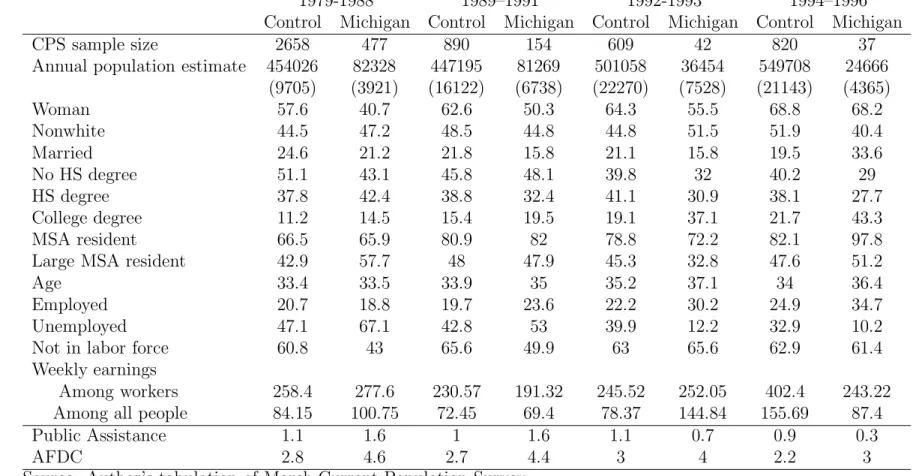
As a response to fiscal pressures in the early 1990’s, many state governments began to cut spending on social welfare programs in general, and General Assistance in particular.5 The elimination of the GA program in Michigan was the most dramatic of all the early welfare reforms in terms of the number of people affected and the amount of lost benefits. Able–bodied adults without children lost all benefits. Families with dependent children were allowed to receive benefits under the new State Family Assistance program. Approximately 9,700 families were thought to be eligible for this program, though actual participation was about half that.6 Adults who had been disabled for at least ninety days and had not qualified for SSI were placed in the new State Disability Assistance program. The average monthly caseload in 1992 was 8,253. For most people SDA benefits were given as interim assistance until SSI benefits were approved. In sum, then, about 82,000 people – or eighty–four percent of the original caseload – lost all benefits in Michigan as a result of the October, 1991 reforms. The top panel of Table (1) presents sample means from the March CPS for people aged sixteen to fifty–four who received income in the previous year from non–AFDC public as-sistance.7 The table is divided into four time periods, 1979 to 1988, 1989 to 1991 (the pre–reform period used in this study), 1992 to 1993 (the post–reform period), and 1994 to 1996; as well as by those who lived in Michigan and in the control states. The first statistic is the sample size for each column. Importantly, and expectedly, the number of Michigan residents in the data who report income from non–AFDC public assistance drops consider-ably in the last two time periods. The second line uses the March CPS sample weights to

4_{Figures are from Department of Social Services, State of Michigan (1990). The AFDC figures refers to}

both Family Groups and Unemployed Parent participants.

5_{For a summary of such policy changes at the state level see Shapiro, Sheft, Strawn, Summer, Greenstein}

and Gold (1991) and Lav, Lazere, Greenstein and Gold (1993).

6_{Federal waivers were granted to Michigan in 1992 that allowed the state to change its AFDC eligibility}

criterion. This allowed many participants of the SFA program to enroll in AFDC.

7_{This assistance could, however, come from sources other than GA. The term “Public assistance” is used}

to refer to any non–AFDC program, while “General assistance” is reserved for that specific program. Note, some people report income from both non–AFDC public assistance and from the AFDC program. Such people are included in Table (1).

estimate how many people this sample represents per year. The 81,269 estimated average public assistance population in Michigan in 1989 through 1991 is about twenty percent below what administrative records indicate the population to have been.8 In the two years after the reform the number drops to 36,454 people. These remaining recipients may have been placed on the medical assistance program that began in 1991, or were originally on a public assistance program other than General Assistance.

The composition of the Michigan public assistance group changed relative to those in the control states in ways that conform to what would be expected from the elimination of benefits for able–bodied adults: The residual programs maintained or created were meant to serve the disabled and those with dependent children. The most telling statistics in Table (1) to this effect are that the proportion of public assistance recipients with a college degree in Michigan jumped from 19.5% in 1989–1991 to 37.1% in 1992–1993. This doubling was far greater than the increase in the control states, from 15.4% to 19.1%. As well, from 1989 to 1993 there was a large change in the labor force status of those on public assistance. Before the General Assistance program was eliminated, about half of public assistance recipients in Michigan were in the labor force and about one half of recipients in the labor force were unemployed. After the GA program was eliminated, however, the remaining public assistance recipients in Michigan were far more likely to be out of the labor force (65.6% in 1992–1993) and very few of those in the labor force were looking for work: their unemployment rate was 12.2% percent after 1992.

The bottom panel of Table (1) gives the percent of all people sampled who report income from AFDC and from non–AFDC public assistance. Public assistance recipiency drops from 1.6% to 0.7% in Michigan, while it rises from 1.0% to 1.1% in other states.

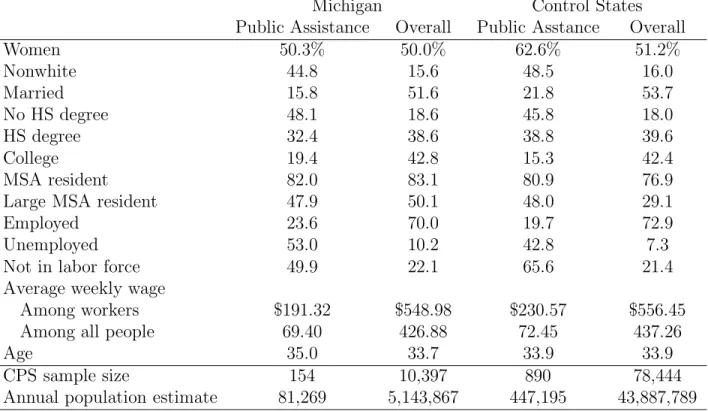
Table (2) compares the characteristics of public assistance recipients to the overall pop-ulation in each state.9 In both Michigan and the control states, public assistance programs

8_{According to the State of MichiganAssistance Payment Statistics, in September, 1991, there were 99,930}

open General Assistance cases in the state. It is likely that the Current Population Survey undercounts those most likely to have been on GA, but is able to accurately count those who remain on public aid after the benefits are terminated for able–bodied adults. The sampling error for these population estimates is also quite large. Blank (1997) finds that the CPS counts only about seventy–five percent of AFDC cases, which is consistent with the undercount found here.

9_{Due to the small sample size for the Michigan public assistance group, the means presented here are}

generally serve non–married and poorly educated individuals, as expected. Interestingly, the proportion of public assistance recipients who live in a Metropolitan Statistical Area (MSA) in Michigan is the same as the population as a whole, approximately eighty–two percent.

3

Literature Review

Previous work offers only limited guidance on the magnitude of wage and employment changes that would result from the increased labor supply of former welfare recipients. The few studies of the labor market effects of federal welfare reform take supply and demand elasticities from previous work outside the area of welfare and welfare reform and use this to construct estimates of employment displacement and wage changes derived from a simple supply and demand framework.10 The difficulty in drawing credible inferences from this work is that labor supply and demand elasticities for very low skilled workers (and unmarried mothers in the case of federal welfare reform) may not be the same as those estimated for workers in general. For example, although most studies tend to find that labor supply among all workers is not very responsive to wages, Juhn, Murphy and Topel (1991) provide evidence that this may not be true among very low–skilled workers. A recent survey of several methodologies by Bartik (1998) examines how labor markets have been affected by federal welfare reform measures between 1996 and 1998, and concludes that declines in wages among female heads of household are likely to be small.

Closely related to the labor market effects of welfare reform is how labor markets re-spond to the influx of new, largely unskilled, immigrants. Card (1997), to cite one example from this literature, argues that immigration in the 1980’s to American metropolitan areas had minimal effects on the earnings of native–born workers. Though small employment dis-placement effects are found, the results suggest that labor demand may be quite inelastic.11 Also related to the elasticity of labor demand is the employment effect of increases in the minimum wage. Recent work by Card and Krueger (1995) argues that there was little em-ployment displacement following recent increases in the federal and state minimum wages,

10_{See for example Mishel and Schmitt (1995) and Bernstein (1997).}

11_{Other studies of the effect of immigration the labor market are Borjas, Freeman and Katz (1992) and}

which suggests that labor demand may be elastic.

4

A Simple Model of Welfare Reform

This section presents a simple model that illustrates some of the important effects that could be expected from the elimination of a welfare program in a local economy.12 Welfare recipients tend to be among the lowest skilled in the population. To draw out the conse-quences of this fact, a key feature of the model is the allowance for a heterogeneity of skills across the population. This heterogeneity leads to a differential impact of welfare reform on people of different skills throughout the local labor market.

Consider a local labor market in which there are _N people working and a group of size

dN people on welfare. Welfare recipients are assumed not to work. There are two prices for labor in the economy,_ws for skilled labor andwu for unskilled labor. Individuals vary in the

amount of skill they have; each person is assumed to have one unit of unskilled labor and

αi units of skilled labor. Thus an individual’s wage is given by wi = wu +αiws. Welfare

recipients earn a benefit of _Bi.

The demand side of the market is specified as simply as possible, while allowing changes in income that result from welfare reform to affect product demand. There are two goods in the economy: a locally produced good, which is sold locally and exported, and a numeraire national good. Export demand for the local good is assumed to be perfectly inelastic. Firms in the local economy operate with identical constant returns to scale production technology, summarized by the unit cost function_c(_{wu, ws, r}). Capital is assumed to be perfectly flexible and readily available at the interest rate _r. The local sector is perfectly competitive, and thus the price of the local good is equal to marginal cost.

Firms in the industry demand skilled and unskilled labor, and hire people with combina-tions of these qualities. Demand for unskilled labor units is given by_Du =_y·_c1(_{wu, ws, r}), and for skilled labor units is given by _Ds = y·c2(wu, ws, r).13 Individuals supply Li(wi, p)

units of unskilled labor, and _αiLi(_{wi, p}) units of skilled labor. Labor market equilibrium is

12_{See Appendix (A) for the details and solution of the model. Studies by Altonji and Card (1991) and}

Johnson (1998) examine similar models in the context of the effects of immigration.

13_c

given by the equality of the supply and demand for each type of labor. By Walras’ law the market for the imported good is in equilibrium.

Let_δl = PNLl i=1Li

be the ratio of the unskilled labor supplied by person_l to the pre–reform stock of unskilled labor. Similarly, let_βl = PαlLl

N i=1αiLi

be the ratio of the skilled labor supplied by person_lto the pre–reform stock of skilled labor. Thus, the sum of_δlandβltaken over the

former welfare recipients (denoted by _j =_N + 1 to _N +_dN) gives the increase in unskilled and skilled labor added to the local economy as a result of these former recipients entering the labor market. Also, denote by_φl = P xl

N+dN k=1 xk

the share of total output bought by person

l. The elasticity of the demand for locally produced output with respect to income is _γw.

The elasticity of labor supply with respect to the wage rate is _w; and with respect to the price of locally produced output is p. Finally, letθn be the share of total costs paid by the

firms to labor type_n.

A base case for evaluating the effect of welfare reform ignores labor supply effects (p =

w = 0), any demand effects on the local product market (γw = 0), and assumes welfare

recipients do not contribute to the pool of skilled labor (PN_j=+_NdN_+1βj = 0). In this case the level

of output and employment is exogenous in equations (16) and (17), and the proportionate change in wages depends only on the uncompensated elasticities of labor demand and the proportionate increase in unskilled labor:

dws ws = " −ηsu ηuuηss−ηsuηus #_N+dN X j=N+1 δj (1) dwu wu = " ηss ηuuηss−ηsuηus #_N+dN X j=N+1 δj (2)

where_ηnm is the uncompensated elasticity of demand for labor of type_n with respect to the wage of type_m. If there are no cross–price effects (_ηsu =ηus = 0), then the skilled wage rate

is unchanged by the addition of unskilled workers to the labor force, and unskilled wages change by the inverse of the elasticity of demand for unskilled labor. Otherwise, nonzero cross–price elasticities introduce feedback between the market for skilled and unskilled labor. Unskilled wage rates will decrease with the addition of unskilled labor to the economy, while skilled wages can increase or decrease, depending on the sign of _ηsu.14

14_{Unskilled wages will unambiguously decrease as long as η}

uuηss−ηsuηus is positive, which is likely as

If there are product demand and labor supply effects, and the welfare population con-tributes to the stock of skilled labor, then the changes in wages take the more general forms:

dws ws = P jβj −γw P jφjwj_B−_jBj λuu−Pjδj−γw P jφjwj_B−_jBj λsu λssλuu−λusλsu (3) and dwu wu = P jδj −γw P jφjwj_B−_jBj λss− P jβj −γw P jφjwj_B−_jBj λus λssλuu−λusλsu (4)

where the summations over _j are over the former welfare recipients, _j =_N + 1 to _N +_dN. The terms in parentheses, therefore, are the proportionate increase in skilled (P_jβj) and

unskilled (P_jδj) labor supplied by former welfare recipients, less their change in product demand brought about by their change in income. The four terms labeled_λmn translate this net impact by the former welfare recipients into changes in skilled and unskilled wages. These depend on the uncompensated elasticity of labor demand and supply, and the elasticity of the demand for output.

The consideration of local product demand effects leads to two complications: first, as welfare recipients’ benefits are replaced by wages, their (positive or negative) change in income affects their demand for output, and this feeds through to firms’ demand for labor. If a substantial number of welfare recipients find jobs and thus increase their income and product demand, the increase in labor demand that results will partially offset the downward wage pressure brought about by the initial increase in labor force participation. Alternatively, if welfare recipients’ income falls (either because they fail to find a job or their wages are lower than their previous benefits) the resulting decrease in product demand will exacerbate the downward pressure on wages. A second product market effect arises because the change in earnings of workers already in the labor market prior to the reform affects their product demand. This feeds back into firms’ demand for labor and equilibrium wages.

The change in employment among people already in the labor market prior to the welfare reform is obtained by differentiating the individual labor supply function, _Li(_wi, p), and

substituting in the changes in wages and prices. The change in labor supplied to the low– skilled labor market is

dLi Li = (wwu wi +pθu)dwu wu + (wαiws wi +pθs)dws ws (5)

Elastic labor supply with respect to wages implies that people will work less when their wage falls. When wages fall, however, the price of locally produced output also falls. This could be thought of as a rise people’s income and, if_p is positive, also lead people to work fewer hours.

To get an idea of the magnitude of the wage and employment changes that welfare reform in Michigan is likely to produce, equations (3), (4), and (5) are simulated using data on Michigan residents in the 1990 Current Population Survey. Hourly earnings are constructed as the ratio of reported weekly earnings to reported hours worked in the week prior to the interview.15 The sample contains all civilians aged sixteen to fifty–four with nonmissing hourly wage data. Observations with hourly earnings less than $2 or greater than $100 per hour (all values are in 1995 dollars) are dropped, leaving a sample of 6562 observations. The average wage among all people is $15.45, and among people without a high school degree is $10.57, eighty–two percent higher than the minimum wage of $4.96. The twenty–fifth, median, and seventy–fifth percentiles are $8.21, $12.87, and $19.92.

For the simulations, the unskilled wage rate is set at the tenth percentile of the wage distribution in Michigan, $5.80. The skilled wage rate is set at the ninetieth percentile of the wage distribution, $27.70. Individual’s level of skill is then given by _αi = (Hourly wage− $5_.80)_/$27_.70.16 Welfare recipients’ benefit is set at the average monthly grant per person in Michigan prior to the elimination of the program, $180 per month. Recipients are assumed to earn $450 per month (which is what someone makes who earns $5.80 per hour and works 20 hours per week for four and a half weeks), if they work, when benefits are eliminated. All former welfare recipients are assumed to be unskilled (_αi = 0).

Other parameters of the simulation are set as follows: the share of total costs paid to all labor is assumed to 70%. The share of total costs paid to unskilled labor (_θu) is 44% and the share paid to skilled labor (_θs) is 26%. The elasticity of demand for locally produced

output with respect to its price is -0.5, and is 0.5 with respect to earnings. The elasticity of labor supply with respect to product prices is assumed to be zero. The elasticity of labor

15_{Questions about usual earnings are only asked in the fourth and eighth monthly interviews; these are}

the so–called Outgoing Rotation Groups. See section (5) for details.

16_{Workers who earn less than $5.80 an hour are assigned a skill level ofα}

supply with respect to earnings is simulated at zero and 0.4. The own–partial elasticity of substitution for each type of labor (_σlland _σss, see appendix) is simulated at -15, -5 , and -1; and the partial elasticity of substitution between skilled and unskilled labor (_σsu and _σus) is simulated at -0.75, -0.25, 0, 0.25, and 0.75. The size of the GA caseload is assumed to be 2% of the state population, though only half of these are assumed to work after benefits are eliminated. Thus potential earnings by former welfare recipients are discounted by half.17

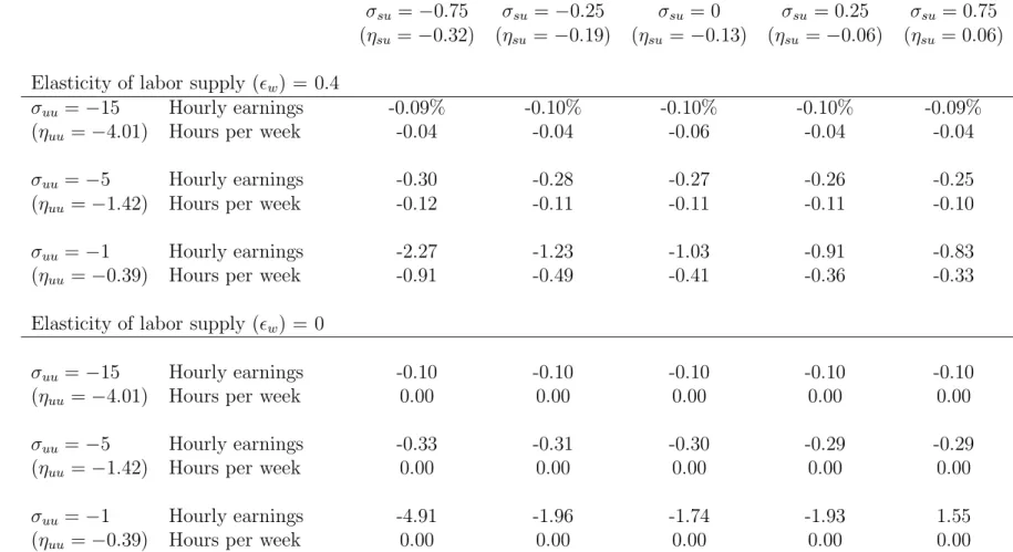
For a given set of parameter values, changes in the skilled and unskilled wages are sim-ulated. Then, using the distribution of the skill parameter from the sample of people from Michigan, changes in hourly earnings and weekly hours among high school drop–outs in Michigan are presented in Table (3). The top panel presents results where the elasticity of labor supply with respect to earnings is 0.4. The columns represent alternative choices of the partial elasticity of substitution between skilled and unskilled labor, ranging from -0.75 to 0.75. Below these, in parenthesis, are the corresponding values of the elasticity of the demand for skilled labor with respect to the price of unskilled labor. The rows repre-sent alternative choices for the own partial elasticity of substitution, with the corresponding elasticity of demand for unskilled labor given in parentheses.18

The most important thing to note from the results is that the simulated changes in hourly earnings and weekly hours of work are very small: for_σuu equal to -15, which corresponds to an elasticity of demand for low–skilled labor of -4.01, hourly wages of people without a high school degree fall by only one tenth of one percent. For _σuu equal to -5, wages still only fall by about one quarter of one percent, with little variation among alternative choices of the elasticity of substitution of skilled and unskilled labor. In both of these cases the changes in hours worked per week are also close to zero.

Significant decreases in the hourly wages only come about when labor demand is very inelastic, as seen in the third row of the table. When skilled and unskilled labor are relative

17_{To simplify the simulation, the share the output purchased by an individual,φ}

l, is assumed to be equal

to his share of the total labor income, P wl N+dN k=1 wk

. Thus the termPN_i=1φ_iwu

wi simplifies to

¯

wu

¯

w ×N+NdN, the

ratio of the unskilled wage to the average wage, times fraction of the population working prior to the welfare reform. Similarly for the analogous term involving skilled wages. This assumption also simplifies the term PN+dN j=N+1φjwj_B−_jBj to ¯ wj−Bj ¯ w ×NdN+dN.

18_{The elasticities of demand depend on other parameters in the model and are given here only for ease in}

substitutes (_σus equal to -0.75, in the first column), hourly earnings among people without

a high school degree would fall by 2.27 percent and hours worked per week falls by 0.91 percent. The decrease in wages and hours worked is smaller the larger is the elasticity of substitution.

The second panel presents results where the elasticity of labor supply is set to zero. As in the top panel, the decrease in wages is very close to zero for _σuu equal to -15 and -5. For the case of very inelastic labor demand, wages fall by about twice as much as in the case of slightly elastic labor supply (though in the case where _σus equals 0.75, wages actually increase).19

Thus, significant decreases in hourly earnings would only be expected if the demand for labor is quite inelastic and skilled and unskilled labor are good substitutes. The intuition behind this result is, at least in these simulations, former welfare recipients supply only unskilled labor, while the average person with a high school degree derives about thirty percent of his income by supplying skilled labor. This supply of skilled labor, the price of which is largely unaffected by welfare reform, acts to buffer the decline in earnings among typical workers in this group.

5

Data

The data used to evaluate changes in economic outcomes in Michigan are from the monthly Current Population Survey. Each household in the CPS sample is interviewed for four months, then ignored for eight months, and then interviewed for the next four months (corresponding to the same four months of year they were interviewed the previous year). In each interview respondents are asked about their current labor force status; however, only in their fourth and eighth interview are they asked about their usual weekly earnings. Respondents are asked about annual income and its sources, including welfare and general assistance participation, only in the March Supplement to the CPS.

Because the effects on the Michigan labor market from the elimination of General

Assis-19_{In simulations (not reported) where the elasticity of demand for output is zero with respect to both its}

price and personal earnings, the fall in wages is slightly larger than those reported here, but the general pattern of the results is unchanged.

tance are likely to affect a small portion of the population, there is a premium to having a large sample in order to obtain as precise estimates as possible. Thus unlike most studies that use the Current Population Survey, this work uses all eight interviews in which respondents participate.20

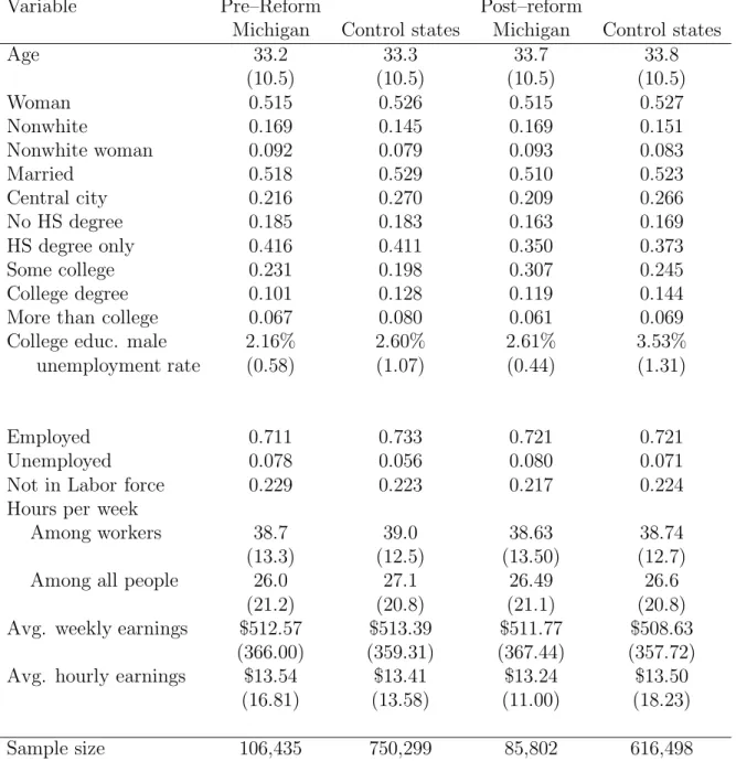
All civilians aged sixteen to fifty–four, who are not self–employed, are used in the estima-tion. Observations with hourly earnings below $2 per hour (1995$), or with weekly earnings data but missing hours, are also dropped from the sample. Table (4) presents sample statis-tics for the variables used in the analysis, broken down by whether the person resided in Michigan and whether they were interviewed prior to October, 1991. The top panel of the table indicates there are few differences in the covariates between people in Michigan and those in the control states.21 The proportion of nonwhites is slightly higher in Michigan; the proportion of the population with a college degree or more education is slightly lower. Although the influence of these covariates are controlled for in the model, had they differed substantially between Michigan and the control states it may signal that the latter is not a good indicator for how the economy of Michigan would have evolved in the absence of welfare reform.

The bottom panel of Table (4) gives the means of the various dependent variables. A person is employed if they worked for a wage any time during the previous week. Labor force participation is defined as some either working or looking for work (unemployed). Two measures of hours of work are examined: hours worked last week among workers and among all people. The former is a measure of the extent of part–time versus full–time work; the latter is a measure of total work effort, which includes transitions into and out of employment. Finally, respondents are asked about their weekly earnings. From this, hourly earnings is calculated as the ratio of weekly earnings to the number of hours worked last week. Both wage measures are deflated to 1995 dollars. In the empirical work below, the log, rather than the level, of weekly and hourly earnings used.

In Michigan the employment–to–population ratio increases after the reform by one

per-20_{Since questions about earnings are only asked in two of the eight interviews, estimates of changes in}

earnings are based on a smaller sample.

21_{The difference in educational attainment between the two time periods are due to changes in the CPS}

centage point, from 71.1% to 72.1%. In the control states employment fell by 1.2 percentage points, from 73.3% to 72.1% of the population, after October, 1991. If in the absence of wel-fare reform in Michigan the employment rate would have dropped by 1.2 percentage points as well, a simple estimate of the effect of the reform on employment is that it led to a 2.2 (= 1.0 - (-1.2)) percentage point point increase in employment in Michigan. Similar calculations indicate that the unemployment rate was 1.3 percentage points higher, and weekly earnings were $3.96 higher in Michigan than they otherwise would have been. These estimates are not, however, credible estimates of the effect of the elimination of the GA program, since there were likely other differences between the labor market in Michigan and in the control states. In particular, there may have been changes in the demand for labor.

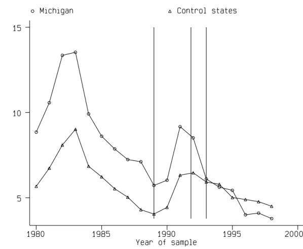
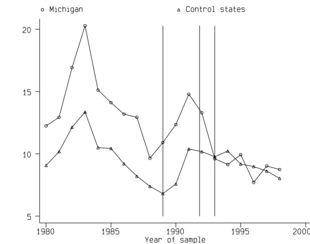
Figures (1) and (2) plot the unemployment rate in Michigan and in the control states from 1980 to 1998.22 The first graph is the rate among all people aged sixteen to fifty– four, while the second is the rate among those without a high school degree. The vertical lines in each graph indicate the pre– and post–reform periods used in this study. The unemployment rate followed similar trends in Michigan and in the control states, though with a level difference between the two. Beginning in 1991, with recovery from the recession, this level difference disappears as unemployment falls faster in Michigan than in the control states. This pattern holds among high school drop–outs as well. Changes in the economy of Michigan other than the elimination of GA benefits were taking place. A simple comparison of changes in employment and unemployment does not identify the effect of welfare reform. The identification procedure in section (6) controls for these differences in labor demand across states, and across skill groups within states.

6

Econometric Specification

The effect of the elimination of General Assistance on labor markets in Michigan is identified by comparing the changes in wages, employment, unemployment, labor force par-ticipation, and hours of work in Michigan with changes in eleven comparison states that did not reform their General Assistance program in the two years after Michigan’s reform.

Since economic conditions are likely to have differed in Michigan and the control states, an important feature of the identification method is that the effects are estimated conditional on the demand for labor of people of different observable skill groups, based on their age, education, and gender. These characteristics are meant to group together people who are likely to be affected similarly by economic shocks. The age groups are sixteen to twenty– nine, thirty to thirty–nine, and forty or older. The education groups are those without a high school degree, those with high school degree only, and those with any post–high school education. With gender, these form eighteen distinct groups.

The outcome of person _i, in group _j, state _s, at time _t, is modeled as

wijst =xijstλ+djst +ijst (6)

where _xijst is a set of covariates that are correlated with economic outcomes; _djst is the average outcome of people in group _j, state _s, at time _t; and _ijst is an unobservable term that reflects individual attributes that influence economic outcomes. Since the skill groups already break the sample into education, age, and gender cells, the covariates (_xijst) include a spline in age and its square within each of the three age ranges, as well as indicators for people who have a college degree and those with any post–graduate education. Also included are indicators for people who are married, nonwhite, both married and nonwhite, and for those who live in a central–city area.23 An ordinary least squares regression of equation (6) produces estimated average outcomes, ˆ_djst, among people in each skill group–state–time cell,

conditional on the individual covariates.

The effect of increased labor market participation by former General Assistance recipients is measured by changes in the average outcomes of groups in Michigan after October, 1991. Thus ˆ_djst is modeled as

ˆ

djst =cj +αjs+βjt+δjst+γjsUst+yt+ξjst (7)

where _cj is a group effect, _αjs is a state and skill group effect, _βjt is a time and skill group

23_{That is, with the subscripts suppressed, the covariates are specified asxλ=age}

1λ1+age21λ2+age2λ3+

age2

2λ4+age3λ5+age23λ6+(College degree)λ7+(Post–grad ed.)λ8+(Married)λ9+(Nonwhite)λ10+(Married×

Nonwhite)λ₁₁+ (City)λ₁₂, where age₁ is equal to the difference between the individual’s age and the mean age among people less than thirty, if the individual is less than thirty, and zero otherwise. Similarly forage₂ andage₃ for those in the other two age groups.

effect, and _δjst is the treatment effect. Ust is the unemployment rate among men in state s

at time _t, which captures business cycle influences on group outcomes. People in different skill groups and states vary in their responsiveness to changes in the overall unemployment rate, which is captured by the loading factor _γjs. Finally, _yt is a time fixed effect, which reflects trends in outcomes among all people, as well as sample design differences in the CPS from year to year. _ξjst is an error term that represents unobservable influences on average economic outcomes, as well as sampling error in the estimation of the cell means.

The treatment effect in equation (7) is implemented as an indicator for people who lived in Michigan after October, 1991, when the General Assistance program was eliminated. Since

αjs captures permanent differences in the level of outcomes between each group in Michigan

and the corresponding group in the control states, and _βjt captures changes in outcomes

of each group across both Michigan and the control states, the treatment effect measures how much average outcomes for groups in Michigan differed after the elimination of the GA program from what they would have been had their change been the same as those groups in the comparison states, controlling for differences in labor market effects, _γjsUst. This

method is implemented in specifications (1) and (3) in Tables (5) and (6), discussed in more detail below.

If there are no other effects specific to the labor market in Michigan after October, 1991, other than those captured by _γjsUst, then the OLS estimate of δjst in equation (7) is

an unbiased estimate of the effect of the elimination of the GA program on labor market outcomes. Put differently, the unobserved influences on economic outcomes, captured by the error term, _ξjst, must be uncorrelated with _δjst.24 Particularly because the unemployment rate in the state may not capture all differences in labor market conditions between Michigan and the control state, this assumption may be overly restrictive. Three less restrictive assumptions about the error term give rise to alternative, unbiased estimates of the treatment effect.

One generalization is to model the unobservable term as having a component that affects

24_{In addition, it is assumed the state policy to eliminate the GA program was not itself related to changes}

in labor market outcomes in Michigan, and that savings in the state budget were not put back in the economy in a way that would effect labor markets.

all groups in a state at a particular time, as well as a random component unique to each group–state–time cell. Specifically,

ξjst =θst+ηjst (8)

Unlike the labor market effects captured by the unemployment rate, the state– and time– specific shocks captured by_θst affect all groups in the state equally. If it is assumed that the

elimination of the GA program in Michigan did not affect the average labor market outcomes of workers with a high school degree or more education, then the treatment effect on workers without a high school degree can be estimated as the difference in average outcomes among the lowest educated group and those with more education, relative to this difference among people in the control states. Because of the large number of better educated people in the Michigan, and the fact that former GA recipients would have likely taken very low–skilled jobs, it is reasonable to assume that only the average outcomes of people without a high school degree would be affected by GA reform. The difference in outcomes among better educated people in Michigan and the comparison states is thus a measure of _θst.

To implement this difference estimator, define _ej to be an indicator that group _j is composed of people without a high school degree. Interactions between_ej and _αjs, _βjt, and

δjst are included in equation (7):

ˆ

djst =cj +αjs+βjt+δjst+ejα0js+ejβjt0 +ejδjst0 +γjsUst+yt+ξjst (9)

where _α0_js, _βjt0 , and _δjst0 capture the differential effects among people without a high school degree. The treatment effect is now the term _ejδjst, which measures the change in labor market outcomes among the least educated groups relative to the change among better educated people, in Michigan relative to the control states. In the empirical implementation, given in specifications (2) and (4) in Tables (5) and (6), groups composed of people with some college education are dropped from the model and the treatment effect is estimated as the difference in outcomes between high school drop–outs and people with only a high school degree.25

25_{People with some post–high school education are dropped since their labor market may be quite distinct}

An alternative to the assumption that the unobservable shock _θst in equation (8) affects

all groups in the state equally is to assume groups are affected by observable business cycle shocks and unobservable shocks to the same degree. That is, if _ξjst = _γjsθst +_ηjst, then equation (7) can be rearranged to give

ˆ

djst = αjs+βjt+δjst+γjs(Ust+θst) +yt+ηjst

= _αjs+βjt+δjst+γjs(˜θst) +yt+ηjst (10)

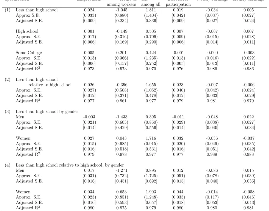
Here the combined shock to each group at time _t in state _s is given by the product _γjs(˜_θst). Since the equation is nonlinear in the parameters, nonlinear least squares must be used. This method is implemented in specifications (1) and (3) in Table (7).

Finally, the two previous cases can be combined to allow for a common unobserved shock to all groups in each state at a particular time, as well as a shock that affects each group by the factor _γjs. That is, the unobservables are modeled as

ξjst =γjsθst +κst+ηjst (11)

The treatment effect is estimated by comparing the change in outcomes of the least edu-cated group relative to those with a high school degree, as in equation (9). When _ξjst is substituted into equation (9), the model becomes nonlinear in the parameters. Results of this specification are given in specifications (2) and (4) in Table (7).

An important assumption of this construction is that the relative demand for people of different skill groups within a state is constant over time (_γjs does not vary over time). This assumption may seem problematic given the well–known decrease in demand for less– skilled labor over the past two decades. If these do not affect Michigan differently than the comparison states, the term _βjt and the time fixed effects will control for the effect of these

changes on the outcome variables. Further, since the estimates below are derived from a five–year time period, any long term–trends specific to Michigan should have only a modest effect on the results.

A number of simplifications are made to the model in equation (7). Rather than represent all eighteen skill groups, the terms _cj, _αjs, _βjt, and _δjst differ only by the three education

classes (less than a high school degree, only a high school degree, or some college education).26 In some specifications the treatment effect, however, will differ by education and gender. In addition, people who live in the control states are treated as if they live in one state, rather than separately identifying each individual state. Finally, the observations are grouped quarterly, rather than monthly, to guard against small cell sizes. With two states, eighteen skill groups, and twenty quarters of data, there are seven hundred twenty cell means ( ˆ_djst).

Finally, use of the quarterly unemployment rate of all men as a proxy for local labor demand raises the issue of the so–called reflection problem. The overall unemployment rate in the state reflects all changes in the local labor market, and in particular any effect from the elimination of the GA program in Michigan. The inclusion of it in the model, therefore, may absorb some of the true variation in labor market outcomes caused by welfare reform. An alternative measure of the local demand for labor is the unemployment rate among college educated men, rather than the overall male unemployment rate. The labor market for higher educated and better skilled individuals would have been affected to a much smaller degree by increased labor market participation among very low–skilled individuals. While this measure is arguably unaffected by welfare reform, it may, however, track changes in the demand for low–skilled labor rather poorly. In addition, because of the smaller number of college– educated men in the data, the unemployment rates are measured with less precision. The results in Table (5) present results of models that use the overall unemployment rate among men, while the models in Table (6) use the unemployment rate among college educated men.

6.1

Estimating standard errors

Efficient estimation of equation (7) requires the use of the full variance–covariance matrix of the skill group–state–time cell means as a weighting matrix. While this matrix can be estimated directly from the residuals of equation (6), because of the unique design features of the Current Population Survey, this is not appropriate in this case. Each individual is observed in the data up to eight times. Particularly because the individual observations are monthly, there is likely to be serial correlation in the unobservable component in equation

26_{That is, α}

js, for example, is implemented as a dummy variable for each combination of the three

(6), ijst. Furthermore, the CPS is a household–level survey. Households are randomly

selected, and all members of the household participate in the survey. Thus, to the extent that individuals within the household jointly determine their employment and hours of work, the unobservable component will be correlated among members of the same household.27

The bootstrap method is used to obtain an unbiased estimate of the variance matrix of the cell means. To mimic the randomization in the CPS sample design, households are drawn with replacement from the set of all households appearing in the data at any time. For each household chosen, all observations associated with that household at any time are included in the dataset. This randomization procedure is replicated fifty times, producing fifty different “random samples” of data, upon which equation (6) is estimated. The empirical covariance matrix of the fifty sets of cell means is an unbiased estimate of the true variance matrix. However, unless the number of bootstrap replications is at least as large as the number of observations (the seven hundred twenty cell means), this estimated variance matrix is not invertible and therefore cannot be used as a weight matrix in a generalized least squares procedure.28 29

A alternative estimation procedure is to use the relative sample size in the each state– quarter–group cell as a weight in a weighted least squares, or nonlinear least squares, esti-mate of equation (7). The standard errors are then computed in a second step using the bootstrapped covariance matrix. The following makes this procedure precise for the lin-ear regression case: let _Z be the (N × K) matrix of explanatory variables in equation (7) and denote as ˆ_D the (N × 1) column vector of the economic outcome under consideration. Equation (7) can then be represented as

ˆ

D=_ZΠ +_ξ (12)

27_{Assortive mating that is correlated with unobserved skills will have a similar effect on the correlation of}

unobservable determinants of wages.

28_{To see this, let c(r) be a column vector of the deviation of the coefficients from the rth bootstrap}

replication from the mean of the fifty coefficients. If there are R bootstrap replications, the bootstrap estimate of the variance–covariance matrix is given byV = (1/R)P_rc(r)∗c(r)0. The rank ofc(r) is one, and thus the rank ofc(r)∗c(r)0 is one. Since V is is the sum of R matricies each with a rank of one, the rank ofV is at most R, and thus not invertible if there less bootstrap replications than the number of cell means.

29_{Even if the estimated variance matrix was invertible, any sampling error in the variance of the cell means}

is correlated with sampling error in the estimated variance matrix. Altonji and Segal (1996) show that this leads to a small sample bias when the inverse of the variance matrix is used as a weight in a GMM procedure.

where Π is the parameter vector and_ξis vector of error terms. _Gis the weight matrix, an (N

×N) diagonal matrix where the_nth diagonal element is the ratio of the number of people in

nth skill group–state–quarter cell to the total number of people in the sample. The weighted least squares estimate of Π is then given by

ˆ

Π = (_Z0_GZ)−1_Z0_GDˆ (13) If there is no specification error in equation (7), and the only source of error derives from sampling error in the estimation of the cell means, then the variance–covariance matrix of those estimates can be used to compute the standard errors of the second stage parameter estimates. Let Σ be the bootstrap estimate of the true variance–covariance matrix of _D, then the variance matrix of ˆΠ is given by

var(Π) = (_Z0_GZ)−1_Z0_GΣ_GZ(_Z0_GZ)−1 (14) Note this is not equal to the variance matrix computed with the weighted least squares formula since Σ does not equal_G−1.30 For the nonlinear least squares models, the matrix _Z in equation (14) is replaced by the matrix of derivatives of the regression equation (10).

7

Regression Results

Tables (5) through (8) present estimation results on the cell means. The first specification in each table presents results for the estimation of equation (6), where the treatment effect,

δjst is stratified by educational attainment. The second specification presents estimation

results of equation (9), which measures the treatment effect on those without a high school degree. The third specification is also based on equation (6), but constrains the treatment effect among those with more education than a high school degree to be zero and stratifies the effect on high school drop–outs by gender. Finally, the fourth specification is analogous to the second specification, but also stratifies the treatment effect by gender.

30_{If there is specification error in equation (7), as well as sampling error in the cell means, computation}

of the correct variance of Π is more complicated and requires additional assumptions about the correlation between the sampling error and the specification error, as well as the correlation in the sampling errors of different cells. When equation (7) is estimated on the individual–level data, rather than the cell means, boot-strapped standard errors are very close to those computed with equation (14), which suggests specification error is not a problem. Those estimates are available upon request.

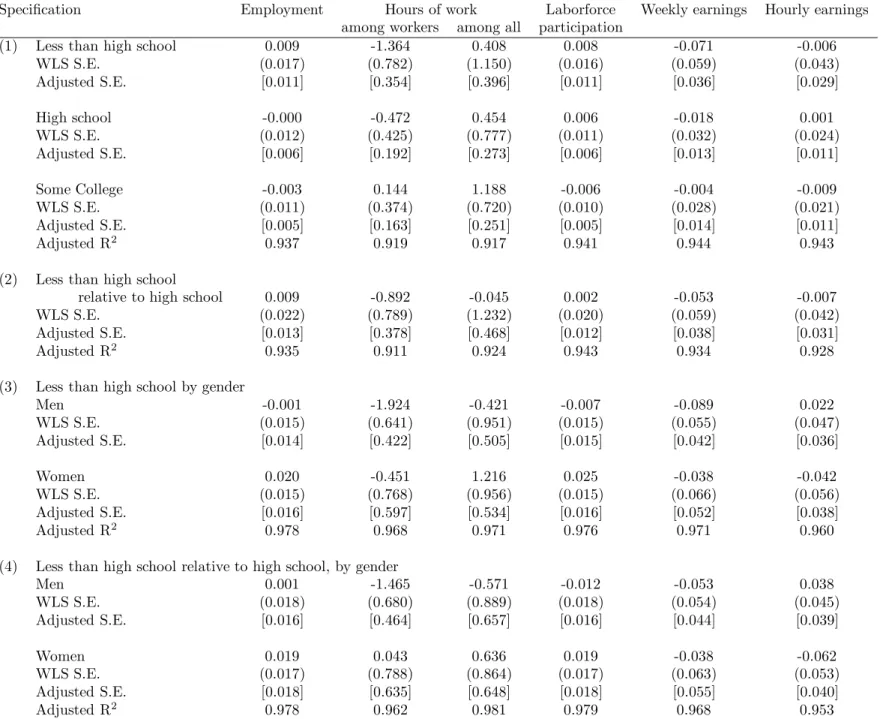
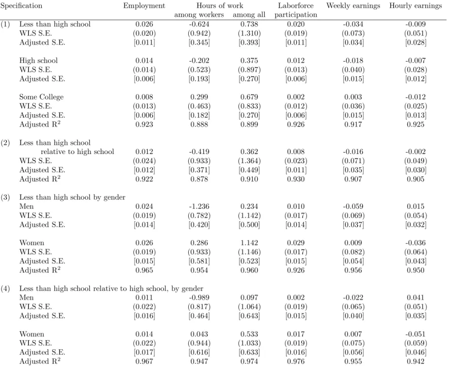
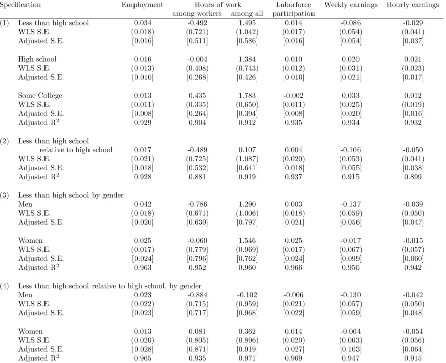
The models in Table (5) use the overall unemployment rate among all men as a control for business cycle effects, while the estimates in Table (6) are conditional on the unemployment rate among college educated men. The results in Table (7) present estimates from the nonlinear least squares models, where _ξjst is specified by equations (10) and (11). Finally, the models estimated using only residents of large MSA’s are reported in Table (8). In these the model is conditional on the unemployment rate of all men in the state, and are thus comparable to the results in Table (5). Below each parameter estimate is the standard error given by the weighted least squares or nonlinear least squares procedure. Below this is the corrected standard error based on equation (14).

Since about half of the GA recipients in Michigan had a high school degree, the estimated increase in employment and labor market participation among high school drop–outs does not estimate the the total increase in these outcomes due to the elimination of the GA program. However, since it is likely that nearly all former GA recipients will enter the very low–skilled end of the labor market, the effects of their increased participation will be more accurately measured by changes in the hours of work and earnings of high school drop–outs in Michigan.

In Table (5), employment among high school drop–outs is estimated to have increased by 0.9 percentage points. There was virtually no change in employment among better educated groups in Michigan, which indicates the model is not picking up alternative influences on the Michigan labor market. Specifications three and four indicate that all of the increased employment was by low educated women. In Table (6), the estimated increase in employment among people of all levels of education is larger when the unemployment rate for college educated men is used as the control for labor demand, which is to be expected since changes in the demand for better skilled people does not perfectly track changes in overall labor demand. The estimated increase among people without a high school degree jumps to 2.6 percentage points. However, if the 1.4 percentage point increase among people with a high school degree is taken as a measure of the labor market shock experienced by everyone in Michigan after October, 1991, the effect of GA reform on the employment of high school drop–outs is only 1.2 percentage points, which is close to the 0.9 percentage point increase from Table (5). Interestingly, the nonlinear models presented in Table (6) show the largest

effect: the estimated increase in employment among high school drop–outs is estimated to have increased by 2.4 percentage points, and no change among better educated groups. As found in Tables (5) and (6), women experienced larger employment gains than men.

The estimates in all three tables indicate that these increases in employment are driven largely by increased labor force participation, though most of the parameters are estimated quite imprecisely. Like the employment estimates, the estimated increases in labor force participation in specification (1) are larger when the unemployment rate among college educated males is used, though when high school drop–outs are compared relative to people with a high school degree, the estimates from Tables (5) and (6) are smaller. In the first table, the estimated increase among high school drop–outs falls from 0.8 percentage points to 0.2 percentage points, while in Table (6) the point estimate falls from two percentage points to 0.8 percentage points. The results in both tables indicate that all of the increase was among low–educated women.

The changes in employment and participation in Detroit (Table (8)) are larger than those for the state as a whole.31 The increase in employment among people without a high school degree was 3.4 percentage points, though labor force participation increased by only 1.4 percentage points. Again these effects are smaller when very low educated people are compared to those with just a high school degree in their state. An important difference, though, between the changes in Detroit and those in the state as a whole is that in Detroit large employment gains were also made by men, not only women. The increase in very low– educated male employment in Detroit was 4.2 percentage points higher than in the control cities (or 2.3 percentage points when measured relative to changes among people with a high school degree). This employment increase among men was largely out of the pool of unemployed workers, as their labor force participation rate was unchanged.

The estimated change in hours of work among workers is largely consistent across all four tables of results, and indicate that hours of work fell among the least educated group, particular among men. When the estimates condition on the overall male unemployment

31_{Since the overall state unemployment rate is used as the control for labor demand in this model, the}

larger effect may simply be due to differing labor market conditions in Detroit. This possibility has not been investigated yet.

rate (Table (5)), the point estimate is that hours among high school drop–outs fell by 1.4 hours per week (or 4% of their average of 33 hours per week). Hours among high school graduates also decreased, however, and thus the relative decline in hours among the least educated in Michigan was only 0.9 hours per week (or 2.7%). In Tables (6) and (7) the decrease in hours worked among workers is slightly smaller, 0.4 hours per week. This decline in hours occurred only for low–educated men, whose average hours declined by one to one and a half hours per week.

In contrast to changes in hours of work among workers alone, changes in hours of work among both workers and nonworkers increased, particularly among female high school drop– outs. The two percentage point increase in employment among women in Michigan found in specification (3), Table (5), corresponds to 1.2 additional hours per week, which is an eleven percent increase from the average of eleven hours per week in this group.32 Since hours per week changed among better educated workers, however, the effect estimated in specifications (2) and (4) are more appropriate estimates of the effect of welfare reform. Low–educated women’s hours increased by only 0.6 hours per week relative to better educated women in Michigan. These estimates are similar when the unemployment rate for college educated men is used to measure business cycle effects. However, the effects are considerably larger in Table (7), when the labor market shocks are treated as unobservable. In that model, increases in overall hours of work among better educated workers are small, 0.5 hours per week for those with only a high school degree, and the increase by low–educated women relative to women with a high school degree (specification (4)) is 1.9 hours per week (or 17% of the average of eleven hours per week). The changes in hours of work in Detroit followed the same pattern as changes among low–educated workers statewide, though the estimated magnitude is smaller.

What emerges from this evidence of changes in labor market participation, employment, and hours of work is that, statewide, women without a high school degree entered the labor market and found work. The magnitude of this increase is between 1.4 and 2.8 percentage points. Increases in employment among men occurred primarily in the Detroit area. As

32_{Since overall hours per week increased among better educated workers (see specification (1)), the}

argued above, the measured increase in employment among the least educated people may understate the overall increase in employment that resulted from the elimination of the GA program, and changes in the hours of work may be a more appropriate barometer of the effects on the lowest skilled people. Overall hours of work among female high school drop– outs increased significantly, most likely due to the employment increases among that group. While most of the models did not find changes in total hours of work among all male high school drop–outs, hours of work among working men in this group declined by between 0.9 and 1.9 hours per week. This could be due to full–time men dropping out of the labor market and being replaced by women and part–time men.

There were about the same number of women as men on GA in Michigan, though the results indicate that only women increased their labor market participation statewide. One explanation for this is that women on GA were, on average, more employable than the men. Support for this comes from a finding by Bound, Kossoudji and Ricart-Moes (1998) that following the elimination of the GA program, SSI applications among men increased signifi-cantly more than those among women indicates that men may have been disproportionately more likely to be disabled. Another explanation for the different finding for men and women is that, although GA recipients lived in Detroit in about the same proportion as the statewide population, the labor market effects by men may have been more pronounced in that city if the availability of low–skilled jobs better suited to men were more concentrated in the city. Finally, displaced men could have chosen to exit the labor market, with the net result of no net increase in employment or labor market participation. On–going work attempts to address these issues.

Since logs of earnings are used as the dependent variables in equation (6), the coefficient estimates in Tables (5) through (8) represent percent changes in hourly and weekly earnings. Statewide, hourly wages among high school drop–outs as a whole did not change. However, the point estimates indicate that hourly earnings rose among the least educated men and fell among women. Conditional on the unemployment rate for all men (Table (5)), relative to the earnings of men with only a high school degree, hourly earnings among men without a high school degree rose by 3.8 percent, and fell by 6.2 percent among women. The numbers are similar in Tables (5) and (6), although in all cases the standard errors are quite large.