econ
stor
www.econstor.eu
Der Open-Access-Publikationsserver der ZBW – Leibniz-Informationszentrum Wirtschaft The Open Access Publication Server of the ZBW – Leibniz Information Centre for EconomicsNutzungsbedingungen:
Die ZBW räumt Ihnen als Nutzerin/Nutzer das unentgeltliche, räumlich unbeschränkte und zeitlich auf die Dauer des Schutzrechts beschränkte einfache Recht ein, das ausgewählte Werk im Rahmen der unter
→ http://www.econstor.eu/dspace/Nutzungsbedingungen nachzulesenden vollständigen Nutzungsbedingungen zu vervielfältigen, mit denen die Nutzerin/der Nutzer sich durch die erste Nutzung einverstanden erklärt.
Terms of use:
The ZBW grants you, the user, the non-exclusive right to use the selected work free of charge, territorially unrestricted and within the time limit of the term of the property rights according to the terms specified at
→ http://www.econstor.eu/dspace/Nutzungsbedingungen By the first use of the selected work the user agrees and declares to comply with these terms of use.
zbw
Leibniz-Informationszentrum Wirtschaft Leibniz Information Centre for EconomicsPickhardt, Michael; Sardà, Jordi
Working Paper
Size and causes of the underground economy in
Spain: A correction of the record and new evidence
from the MCDR approach
CAWM discussion paper / Centrum für Angewandte Wirtschaftsforschung Münster, No. 54 Provided in cooperation with:
Westfälische Wilhelms-Universität Münster (WWU)
Suggested citation: Pickhardt, Michael; Sardà, Jordi (2011) : Size and causes of the
underground economy in Spain: A correction of the record and new evidence from the MCDR approach, CAWM discussion paper / Centrum für Angewandte Wirtschaftsforschung Münster, No. 54, http://hdl.handle.net/10419/55038
A correction of the record and new evidence from the MCDR approach
by
Michael Pickhardt and Jordi Sardà
January 2012
Abstract: We review existing estimates of the size of the Spanish underground economy,
apply the Ahumada et al. (2007, RIW) correction procedure to some of them and calculate the size of the underground economy in Spain for the period 1960 through 2009 by using the modified-cash-deposits-ratio (MCDR) approach recently developed by Pickhardt and Sardà (2011, EJLE). We then extend the MCDR approach with respect to an analysis of the causes of the Spanish underground economy. Contrary to most other studies, we show that the latter is not predominantly caused by tax pressure, but by labor market aspects, macroeconomic influences and criminal activities. Based on these findings we derive some unprecedented policy recommendations.
JEL: O17, H26, C22, Keywords: underground economy, shadow economy, hidden economy, black economy, cash-deposit-ratio, currency demand approach, MIMIC approach,
Acknowledgements: An earlier draft of this paper was presented at the international
conference The Shadow Economy, Tax Evasion and Money Laundering (shadow2011), University of Münster, Germany, July 2011. Sardà gratefully acknowledges financial support by the DAAD (Project A/07/14771), the Comerzbank Foundation and the Spanish Ministry of Education and Science, Project Nr. ECO2010-17113.
Corresponding author:
Michael Pickhardt, Brandenburg University of Technology Cottbus, Department of
Economics, Postbox 101344, 03013 Cottbus / Germany, Tel. (0)355-69-2914, Fax. +49-(0)355-69-4955, E-mail: [email protected]
Jordi Sardà, Universitat Rovira i Virgili, Department d’Economia i CREIP, Av. Universitat 1, 43204 Reus / Spain, Tel. +34-977-759-853, Fax. +34-977-300-661, E-mail:
Size and causes of the underground economy in Spain:
A correction of the record and new evidence from the MCDR approach
1 Introduction
The size, scope and impact of the underground economy1 are among the top issues of the
political and economic policy debates in Spain. Although these debates are fuelled by the
current economic situation of Spain, the day to day presence of underground economy
activities in most people’s social environment also contributes to an increasing awareness.
From a scientific point of view, however, any analysis of the size, scope and impact of the
underground economy is faced with severe data problems because underground activities are
not recorded and anyone engaged in such activities has a strong incentive to hide them.
Therefore, economists have developed a variety of methods to estimate the size of the
underground economy and some of them are discussed in Schneider and Enste (2000),
Kazemier (2006), Pickhardt and Shinnick (2008) or Adair (2011).
Yet, the most frequently applied approaches, the Multiple-Indicators-Multiple-Causes
(MIMIC) method and the currency demand method (the latter is often used as an input for the
MIMIC approach, see Giles 1999), have been heavily criticized on econometric grounds by
Breusch (2005a,b,c,d). In addition, Ahumada et al. (2007) have shown that the currency
demand method produces coherent estimates only if the long run income elasticity of the
demand for currency is equal to unity. A condition that is not fulfilled for various published
estimates. Moreover, Ahumada et al. (2008) have shown that if the lagged dependent variable
is used in currency demand estimations, calculating cardinal values of the size of the
underground economy requires a known initial value of the size of the underground economy.
Again, in a number of relevant published estimates no such initial value was used. To this
1 We use the term ‘underground economy’ interchangeably with terms such as shadow economy, hidden economy, black economy, etc. (see Kazemier 2006, Pickhardt and Sardà 2011).
extent, many estimates of the size of the underground economy have produced faulty figures
and, therefore, have provided misleading information to the public, to politicians and law
makers.
The purpose of this paper is to address this issue in three ways. First, we review existing
estimates of the size of the Spanish underground economy. Second, we apply the Ahumada et
al. (2007) correction to relevant estimates. Third, we apply a rather simple calculation
method, the modified-cash-deposits-ratio (MCDR) approach, which was recently developed
by Pickhardt and Sardà (2011) and which is not subject to the critique of Breusch
(2005a,b,c,d) and Ahumada et al. (2008, 2007). Moreover, we extend the MCDR approach by
incorporating an analysis of possible causes of underground economy activities. Among other
things, we show that the MCDR approach allows for reproducing various existing estimates
of the Spanish underground economy, that some previously published estimates are untenable
with respect to the size of the latter and/or its evolution over time, and that the Spanish
underground economy is predominantly caused by labor market aspects, macroeconomic
issues and illicit activities, rather than just by tax pressure. These findings allow us to draw
some comprehensive and unprecedented policy conclusions for combating the Spanish
underground economy.
The paper is structured as follows. In the next section we deal with the size of the Spanish
underground economy. First, we briefly review previous estimations. We then employ the
Ahumada et al. (2007) correction procedure to some of these estimates. Eventually, we use
the MCDR approach for calculating the size of the Spanish underground economy. In section
three we compare and contrast our findings with previous estimates, provide an analysis of
possible causes of the Spanish underground economy and offer some policy
2 Size and Evolution of the Spanish Underground Economy
Estimates of the size of the underground economy in Spain have been conducted since the
1980s by various researchers. However, almost all of them have used the monetary approach
in one way or another. The latter is an indirect macro-based method that rests on the quantity
theory of money and was pioneered by Cagan (1958). Two decades later, Gutmann (1977)
developed a simple non-econometric calculation procedure based on the monetary approach
and applied it to U.S. data. In contrast, Feige (1979), Klovland (1980, 1984), Tanzi (1980,
1982, 1983), Bhattacharyya (1990), and Escobedo and Mauleón (1991) have developed
variants of the monetary approach that are all based on an econometrically estimated money
demand equation. Therefore, these variants of the monetary method are also known as
variants of the currency or money demand method.
Moreover, as noted, results derived from a monetary method are often used as a calibration
input for MIMIC estimations. This is because the MIMIC method, which was first applied to
underground economy estimations by Frey and Weck (1983), just generates relative estimates,
so that the MIMIC index must be calibrated with a benchmark value taken from another
source in order to get cardinal values of the size of the underground economy (e.g. see Giles
1999, F373; Schneider and Enste 2000). Apart from the monetary approach and the MIMIC
approach, there are a number of alternative methods for estimating the size of the
underground economy, which are reviewed, among others, by Schneider and Enste (2000),
Kazemier (2006) or Adair (2011).
2.1 Previous Estimates
The first estimates of the Spanish underground economy were conducted by Lafuente Félez
(1980), using the Tanzi method and by Moltó Calvo (1980), using the Gutmann method.
(1978) and one percent (1976), respectively. Several other authors have also contributed some
evidence for selected years (see Table 1, column Var.).
A time series of the size of the Spanish underground economy is provided by several
authors who use different variants of the monetary method. For example, Escobedo and
Mauleón (1991), Mauleón and Sardà (1997), Gómez-Antonio and Alañón-Pardo (2004), and
Arrazola et al. (2011) all apply the Escobedo and Mauleón (1991) method. The MIMIC
approach is used by Alañón-Pardo and Gómez-Antonio (2005), who calibrate their MIMIC
model with the 1980 value and the 1980-1981 growth rate of the underground economy
according to Gómez-Antonio and Alañón-Pardo (2004). Dell’Anno et al. (2007), essentially
do the same because they also calibrate their MIMIC model with a 1980 value taken from
Alañón-Pardo and Gómez-Antonio (2005) or Gómez-Antonio and Alañón-Pardo (2004).
Moreover, Weck-Hannemann et al. (1984), Schneider (1997a,b, 2010) and Feld and
Schneider (2010) also provide results for selected years based on a MIMIC model, which is
calibrated with values taken from a currency demand method. In contrast, Prado-Domínguez
(2004) offers a time series derived from using the Tanzi method and Gadea and Serrano-Sanz
(2002) and Serrano-Sanz et al. (1998) provide several time series that are based on the
Klovland (1980, 1984) method. Finally, Arrazola et al. (2011) not only use the currency
demand method of Escobedo and Mauleón (1991), but also the MIMIC method and an
electricity approach that is related to the method of Escobedo and Mauleón (1991).
Hence, almost all available estimates of the size of the Spanish underground economy are
based on a variant of the monetary approach. In Table 1, columns three to 14 (counted from
left to right) give an overview concerning these results, where the size of the underground
economy is measured in percent of the official GDP. Inspection of Table 1 shows that most of
the estimates in columns three to 14 provide fairly close values in several years, but not in all
of them. For example, during the period 1980-1989, where most of the series overlap, the size
of official GDP in 1980 to about 20 percent in the late 1989, although in some years there are
marked differences between the series. Also, during this period all estimates peak in 1989,
except those of Mauleón and Sardà (1997) and Dell’Anno et al. (2007).
To explain these and other differences in the results, we proceed with examining the
estimations in some detail. First, we consider the results in columns three to seven (EM, MS,
GA, A+1, (A+2)), which are all obtained from a direct application of the Escobedo and
Mauleón (1991) variant of the currency demand method, except the A+2 profile, which is
obtained from an electricity demand method that is otherwise based on the Escobedo and
Mauleón (1991) method. The main advantage of the latter is that it does not require the
assumption of equal velocities of money circulation in both the legal and underground
economy, an assumption that is central to all other versions of the monetary approach
mentioned above and, in fact, one of the most heavily criticized assumptions regarding this
approach (e.g. see Thomas 1999). The major disadvantage of this method is that it necessarily
mimics the evolution of the tax pressure variable over time. Essentially, this means that any
underground economy profile obtained from applying the Escobedo and Mauleón (1991)
method cannot represent the evolution of the underground economy over time, unless it
accidentally coincides exactly with the development of the tax pressure variable over time.2 In
fact, this may be clarified by the equation from which an absolute value of the underground
economy is obtained (see Escobedo and Mauleón 1991, 109),
YU,t = (a2 / b1) Tt, (1)
where YU denotes the size of the underground economy in absolute terms, T is the tax
pressure variable, a2 is the coefficientof the tax pressure variable, b1 is the coefficient of the
2 Obviously the same is true if several pressure variables are used as this would just lead to an underground economy profile that represents a combination of the profiles of these pressure variables.
legal size of the economy YL and t is the time index. However, equation (1) applies only in
cases where cash in circulation and legal money are estimated separately. If just a single
estimation is used, equation (1) amounts to,
t , F 1 3 1 t , F 3 t , L t , U P 1 ) / P exp( Y Y
α
α
α
α
⋅ − ≅ = , (2)where PF,t corresponds to the tax pressure variable T, α3 is the coefficient of the tax pressure
variable and α1 is the coefficient of the legal size of the economy YL (see Mauleón and Sardà
1997, 126; Gómez-Antonio and Alañón-Pardo 2004, 14; Alañón-Pardo and Gómez-Antonio
2005, 1016). Hence, equations (1) and (2) make it clear that differences in the results shown
in columns three to six of Table 1 must ceteris paribus come either from different values of
the coefficient ratio and, thus, from running the estimation with different variables, but with
the same tax pressure variable and/or from choosing a different tax pressure variable. Put
differently, if the tax pressure variable is the same, but other variables in the estimated
equation differ, ceteris paribus this would result in a different size of the underground
economy (i.e. a different ratio α3/α1), but not in a different profile over time. We will come
back to this issue in section three.
Next, we consider results shown in columns eight and nine of Table 1 (AG and DGA).
These results indirectly rest on the Escobedo and Mauleón (1991) variant because they are
both obtained from calibrating a mimic index with the 1980 value of column GA.3 This
notwithstanding, the results in columns AG and DGA show a rather different profile and
differ in most years, with up to 15 percentage points (see Table 1, 1997). Differences in the
calibration procedure, underlying mimic indices and, therefore, alternative specifications of
the MIMIC models explain these results. In this context, it seems worth noting that combining
3 As noted, Alañón-Pardo and Gómez de Antonio (2005, 1019) have used, in addition, the growth rate of the underground economy during the period 1980-1981.
the Escobedo and Mauleón (1991) variant with a MIMIC index essentially solves the major
problem of the former with respect to its incapacity of providing a profile that is independent
from the profile of the tax pressure variable (see also Pickhardt and Sardà 2006).
We now turn to columns 10 to 13 of Table 1 (P, GS1, GS2, SE+). These results all differ
with respect to the profile and they differ substantially with respect to the size of the
underground economy, if results from the Tanzi method (column P) are compared to those
obtained from the Klovland method (columns GS1, GS2, SE+). However, these estimates are
subject to a recently proposed correction procedure and, therefore, we refrain from any closer
inspection but turn to the Ahumada et al. (2007) correction procedure.
2.2 Ahumada et al. Correction Procedure
According to Ahumada et al. (2007), the currency demand method may produce coherent
estimates provided that the long run income elasticity of the demand for currency, say β,
equals one, β = 1.4 This condition is an implication of the assumption of equal velocities of
cash circulation in both the legal and underground economy. As noted, it is one of the crucial
assumptions on which the currency demand method rests (e.g. see Breusch 2005b, 396),
except the version developed by Escobedo and Mauleón (1991).
In addition, Ahumada et al. (2007) provide a correction procedure, which can be applied if
the long run income elasticity of the demand for currency differs from unity, β≠ 1. In general,
the Ahumada et al. (2007, 368) correction is:
L U 1 L U Y Y Y Y = β , (3) 4 The condition
β = 1 is generally required, except in the rather unlikely case where the size of the underground economy is exactly equal to the size of the legal economy (see Ahumada et al. 2007, 367).
where YU denotes the size of the underground economy in national currency, YL denotes the
size of the legal economy in national currency, the ratio YU /YL denotes the faulty size of the
underground economy, the ratio YU /YLdenotes the correct size of the underground economy
and β is the long run income elasticity, which is different from unity.
Following Ahumada et al. (2007), we choose to correct the Klovland based estimates of
Gadea and Serrano-Sanz (2002) and Serrano-Sanz et al. (1998), which are shown in columns
GS1, GS2 and SE+ of Table 1, respectively. The three models essentially differ with respect
to the model specifications. The long run income elasticity’s of the demand for currency
regarding these three models are,
β1
= 1.68 (GS1),β2
= 0.52 (GS2) andβ3
= 0.8 (SE+). Then, if we consider the faulty size of the underground economy in a specific year, say 1980 (seeTable 1), which is (YU /YL)1 = 0.0634 in the case of (GS1), application of (3) yields:
0.0634(1/1.68) = 0.19362, which gives a corrected size of 19.36 percent of GDP for the Spanish
underground economy in 1980 (see Table 1, column A-GS1). Likewise, for the second model
we get (YU /YL)2 = 0.0728, which yields: 0.0728(1/0.52) = 0.006483, so that the corrected size
is 0.65 percent of GDP (see Table 1, column A-GS2) and for the third model we get
(YU /YL)3 = 0.0585, which yields: 0.0585(1/0.8) = 0.02877, so that the corrected size is 2.88
percent of GDP (see Table 1, column A-SE+). Corrected values for the entire period are
obtained in the same way and displayed in Table 1, columns A-GS1, A-GS2 and A-SE+,
respectively.
Inspection of Table 1 shows that the corrected sizes of the Spanish underground economy
are substantially different from the initially published sizes.5 Moreover, because all three
corrected estimations are also subject to the critique of Ahumada et al. (2008), even the
corrected values may not give a good approximation of the Spanish underground economy. In
5 Ahumada et al. (2007, 370) correct the estimate of Isachsen and Strom (1985, 24) for Norway, which is also based on the Klovland method and find that the corrected size of the underground economy is 1.51 percent of GDP in 1978, rather than 6.3 percent.
this context it is worth noting again that the Ahumada et al. (2008, 2007) critique also applies
to the results of Prado-Dominguez (2004), column P of Table 1, which are obtained by using
the Tanzi version of currency demand method.
To summarize, inspection of Table 1 shows that applying the Ahumada et al. (2007)
correction procedure leads to a substantial increase in the variability of the results. Given that
these estimates are otherwise correct, the model specification seems to have a much larger
impact than initially though. Yet, even the corrected values may still be faulty according to
Ahumada et al. (2008) and Breusch (2005b,c). In any case, our brief review of existing
estimates demonstrates that there is some faulty and mixed evidence concerning the size and
evolution of the underground economy in Spain. Possible ways of addressing this issue
include developing and applying alternative methods as well as conducting plausibility tests.
Therefore, we proceed with applying the MCDR approach.
2.3 The MCDR Approach
The modified-cash-deposits-ratio (MCDR) approach was recently developed by Pickhardt and
Sardà (2011) with a view to address various issues. First, to circumvent econometrical and
mathematical criticism put forward by Breusch (2005,a,b,c,d) and Ahumada et al. (2007,
2008). Second, to include cash used in illicit economic activities, such as drug dealing, human
trafficking, etc., that are not caused by tax pressure. Third, to simplify plausibility testing with
respect to results obtained from other methods. Fourth, to raise the level of transparency
regarding the estimation procedure.
Essentially, the MCDR approach is a modified version of the original Gutmann approach.
Formal representations and critical reviews of Gutmann’s original approach are provided by
Thomas (1999, F382–F383), Feige (1989, 36–44), and Blades (1982, 43), among others.
According to a central assumption of the original Gutmann approach, agents in the legal
over time. However, despite some country specific differences, agents in industrialized
countries apparently seem to have changed their preferences over time toward a substantially
higher share of deposits. Thus, application of the original Gutmann approach would now
generate negative values of the underground economy in many countries.
Therefore, Pickhardt and Sardà (2011, 149–150) assume instead that “all currency in
circulation in the base year, C0, represents the entire cash agents wish to hold in any year after
the base year for the set of legal transactions they prefer to carry out in cash”. In addition, the
authors assume that all additional transactions in the legal economy are carried out via sight
deposits by using cheques, debit and credit cards, etc., but continue to apply the remaining
assumptions of the original cash-deposit-ratio approach. Thus, by definition, any cash
holdings in excess of those in the base year can be fully attributed to the underground
economy. Subject to these assumptions, Pickhardt and Sardà (2011, 150) show that using
Irving Fisher’s (1911) quantity theory of money leads to:
Ut Lt t t Y Y D C C C = ⋅ + − 0 0 , (4)
with C0 =CLt, andCt – C0 = CUt, t = 1, …, Z, and where Ct denotes currency in circulation
outside banks at the end of the year, C0 denotes currency in circulation outside banks at the
end of the base year or base period, here 1960, CL denotes currency used for legal
transactions, CU denotes currency used for underground economy transactions and Dt denotes
sight deposits held by domestic non-banks (non-MFIs) at the end of the year.
Although this modification solves the major problem of the original cash-deposit-ratio
approach (i.e., negative results), Pickhardt and Sardà (2011, 150–156) emphasize that all
version as well. This notwithstanding, they suggest and apply further auxiliary modifications
that may to some extent address this criticism.
In particular, these auxiliary modifications are (Pickhardt and Sardà 2011, 153): “1) that
inflation may require increasing C0 over time to allow agents to carry out their preferred set of
cash transactions, 2) that changes in the size of the population may require to adjust C0 over
time, 3) that a certain fraction of Ct may be held abroad, 4) likewise, that a certain fraction of
Ct may be hoarded by national agents, 5) that the number and set of transactions, which agents
wish to carry out in cash, may change over time, for example, due to the evolution of new
non-cash payment methods and facilities, 6) that some proceeds from underground activities
may in fact be held as sight deposits, for example, because of money laundering or because
the illegal transactions did not involve any cash payments at all, so that Dt may have to be
reduced accordingly to DLt in the denominator of (4) and DUt may have to be added to CUt in
the nominator, with Dt = DLt + DUt, 7) that the size of the underground economy may not have
been close to zero in the base year or base period”.
In the present paper we have addressed the first two modifications (inflation and
population) and have forecasted Ct for the relevant period to bridge the gap caused by the
Euro introduction (see appendix). Yet, we refrain from applying the third auxiliary
modification because we have no evidence that substantial amounts of Pesetas were held
outside Spain during the period under consideration and we could not apply the remaining
modifications due to a lack of data. Given these auxiliary modifications, (4) changes to (5),
Ut Lt t t 0 t 0 t Y Y D PIC PIC FC = ⋅ + − , (5)
Table 1: Size of the Spanish Underground Economy in Percent of GDP
S2 Year EM MS GA A+1 A+2 AG DGA P GS1 GS2 SE+ Var. A-GS1 A-GS2 A-SE+ 0.00 1960 2.6W 3.06 1961 6.39 1962 7.75 1963 10.01 1964 18.21 3.60 5.86 6.46 13.82 0.43 3.26 10.02 1965 17.91 3.7 5.6 6.14 14.05 0.39 3.06 13.00 1966 17.56 3.8 6.0 6.18 14.28 0.45 3.08 14.68 1967 16.65 3.8 5.6 5.90 14.28 0.39 2.91 15.35 1968 1.7 16.03 3.0 4.5 5.05 12.40 0.26 2.39 16.93 1969 1.6 15.15 3.0 4.1 4.58 12.40 0.21 2.12 17.57 1970 1.8 15.58 3.03 4.57 4.40 12.48 0.26 2.02 16.04 1971 2.6 14.19 2.6 3.6 3.85 11.39 0.17 1.71 15.29 1972 3.9 12.99 2.3 3.4 3.59 10.59 0.15 1.56 14.68 1973 12.3 4.5 12.69 2.3 3.5 3.45 10.59 0.16 1.49 14.12 1974 12.6 4.2 13.16 2.3 3.2 3.34 10.59 0.13 1.43 13.78 1975 14.4 5.3 12.61 2.85 3.67 3.70 12.03 0.17 1.62 13.28 1976 15.3 8.8 7.6 12.37 3.0 3.8 3.73 1.0M 12.40 0.19 1.64 14.27 1977 16.5 10.3 8.7 13.06 3.8 5.8 3.92 6.5W 14.28 0.42 1.74 15.16 1978 17.6 11.7 10.6 13.31 4.0 6.5 4.32 22.9L 14.72 0.52 1.97 13.72 1979 18.5 13.0 12.1 13.82 4.9 7.0 5.80 16.61 0.60 2.85 13.48 1980 3.7 17.9 15.5 11.69 11.69 14.0 15.1 14.26 6.34 7.28 5.85 19.36 0.65 2.88 12.90 1981 5.2 17.9 16.7 12.25 12.50 15.4 18.1 14.33 5.7 6.4 5.89 18.17 0.51 2.90 13.76 1982 6.8 17.1 16.3 12.68 12.69 15.2 20.4 14.96 5.3 5.6 5.63 17.40 0.39 2.74 13.88 1983 9.1 17.1 16.5 13.40 13.94 16.1 22.6 15.50 6.0 7.5 6.80 18.74 0.69 3.47 13.92 1984 10.7 16.2 16.7 12.32 14.17 15.3 24.2 16.15 8.3 8.3 7.39 22.73 0.83 3.85 14.35 1985 13.0 15.7 17.2 11.67 14.93 14.9 27.2 16.91 8.94 9.50 8.45 23.76 1.08 4.56 15.99 1986 14.6 15.5 18.7 9.51 15.84 15.4 28.7 17.34 9.6 8.5 7.98 24.79 0.87 4.24 17.46 1987 16.9 15.7 18.5 13.96 17.02 15.9 28.7 17.59 14.5 14.3 10.41 31.68 2.37 5.91 19.97 1988 18.5 15.7 18.4 13.94 17.11 15.7 26.4 18.40 15.8 16.7 11.44 33.34 3.20 6.65 22.85 1989 20.8 15.9 18.9 17.85 18.27 16.5 24.9 19.86 19.2 21.6 13.69 37.44 5.25 8.33 24.52 1990 16.2 19.8 17.92 18.13 17.2 24.5 19.50 16.1 16.5 12.46 16.1I 33.72 3.13 7.40 30.90 1991 16.7 19.9 18.31 18.32 18.0 24.2 21.05 15.6 16.5 13.64 33.09 3.13 8.29 35.03 1992 18.0 19.4 19.62 18.99 19.0 26.8 24.75 20.02 18.88 15.42 38.39 4.05 9.66 37.84 1993 18.4 20.1 19.61 18.35 18.9 28.7 25.38 21.6 20.1 14.15 40.16 4.57 8.68 40.43 1994 17.8 20.2 18.49 18.38 17.8 32.5 25.58 19.9 17.0 13.97 22.3R 38.25 3.31 8.54 41.64 1995 16.4 20.1 17.31 17.91 16.8 31.2 26.92 18.92 17.36 14.13 22.4I 37.12 3.45 8.66 41.15 1996 16.8 20.0 16.69 17.76 16.1 30.9 26.33 18.3 17.4 36.39 3.46 37.59 1997 20.1 18.05 18.40 15.9 30.9 24.29 18.4 17.5 36.51 3.50 30.67 1998 21.2 17.92 18.62 15.3 29.4 21.79 18.91 16.79 23.1I 37.11 3.23 30.64 1999 20.7 18.73 19.22 15.5 28.7 19.15 26.26 2000 20.9 19.03 19.25 15.9 26.2 18.46 22.7I 22.96 2001 19.22 18.97 16.4 25.7 17.75 21.44 2002 20.16 19.22 18.2 26.3 22.5I 19.82 2003 20.05 19.24 26.4 22.2 18.17 2004 20.85 19.54 21.9 15.55 2005 22.64 20.26 21.3 13.46 2006 24.46 20.86 20.2 14.48 2007 26.37 21.23 19.3 17.76 2008 21.29 18.47 18.7 21.07 2009 19.5 2010 19.8
Note: All values show the size of the Spanish underground economy in percent of legal GDP according to the various authors, except in column year. S2 represents the size of the Spanish underground economy according to the MCDR approach, equation (5), own calculations. EM denotes values of Escobedo and Mauleón (1991, 119). MS denotes values of Mauleón and Sardà (1997, 128). GA denotes values of Gómez-Antonio and Alañón-Pardo (2004, 17). A+1 and A+2 denote values from Arrazola et al. (2011, 93), where A+1 refers to the currency demand model and A+2 to the electricity model. AG denotes values by Alañón-Pardo and Gómez-Antonio (2005, 1020). DGA denotes values of Dell’Anno et al. (2007, Table 6, 69, for years 1990, 1995, and 2000, with the remaining values read from Fig. 4, 68, which are, therefore, denoted in italics). P denotes values of Prado-Domínguez (2004, 440). GS1 and GS2 denote values of Gadea and Serrano-Sanz (2002, for years 1964, 1970, 1975,
1980, 1985, 1992, 1995 and 1998 from Table 4, 514, all other values are read from Figure 4, 515, with respect to DIR2 (GS1) and DIR2 with neither INNOV nor PDP variables (GS2). SE+ denotes values of Serrano-Sanz et al. (1998, 32). Var. denotes values by various authors: W denotes values of Weck-Hannemann et al. (1984), cf. Schneider (1997a, 43; 1997b, 140), where 6.5 actually refers to 1978, M denotes Moltó Calvo (1980, 51), L denotes Lafuente Félez (1980, 590), R denotes Schneider (1997b, 149), I denotes Feld and Schneider (2010, 134), where the values represent the average between the selected year and the previous one, and with respect to 2003 to 2010 values are taken from Schneider (2010, 3)). A-GS1, A-GS2 and A-SE+ denote the Ahumada et al. (2007) correction applied to the values of GS1, GS2 and SE+, respectively (own calculations).Underlined numbers indicate the peak of the series and numbers set in italics denote that these numbers were read from figures.
Figure 1: Size of the Underground Economy in Spain (S2) and Germany (G3) in Percent of GDP based on MCDR approach
Note: S2 profile, own calculations. G3 profile obtained from Pickhardt and Sardà (2011,
151-152).
where FC denotes forecasted currency in circulation outside banks and PIC0 denotes
population and inflation adjusted values of C0. Hence, according to (5) it is assumed that on
legal transactions in cash. Of course, the qualifications made by Pickhardt and Sardà (2011,
155–156) with respect to this notion, the changes in the statistics of sight deposits due to the
Euro introduction and regarding the base year apply here as well. Then, application of (5) to
the Spanish data set yields the size of the Spanish underground economy according to the
MCDR approach, which is displayed in column S2 of Table 1. In Figure 1 we display and
contrast the Spanish underground economy profile S2 with the German underground economy
profile G3, which Pickhardt and Sarda (2011) have calculated using the MCDR approach.6
Although the same approach and the same period have been used the two profiles differ
remarkably, with the German profile being always below the Spanish one.
To summarize, by applying the MCDR approach to Spain we obtained underground
economy profile S2. Yet, despite the fact that additional modifications are considered
necessary, relevant data is currently unavailable so that further quantitative adjustments are
impossible. Moreover, because these additional adjustments may have different signs, the sign
of the net effect is unpredictable. Therefore, the S2 profile may represent a lower or upper
bound of the size of the cash using section of the Spanish underground economy, or may even
represent a rough estimate of its true size in case possible other influences balance.
3 Causes of the Spanish Underground Economy
As noted elsewhere, an inconvenience of the MCDR approach is its inability to explain
possible causes of the underground economy. To address this issue, we now extend the
MCDR approach by exposing the S2 profile to an econometrical estimation procedure.
However, we first use a simple correlations test to further examine the profiles of the Spanish
underground economy, as summarized in Table 1.
6
Given some Deutsch-Mark specific circumstances the German G3 profile, rather than the G2 profile, should be compared with the Spanish S2 profile. Also, in Table 1 we directly display the S2 profile, but not the corresponding auxiliary profiles S0, S0_2, S1, as in Pickhardt and Sardà (2011, 151, Table 2, l.h.s.). Moreover, as noted in Pickhardt and Sardà (2011), during the period 1987 to 1991 the G3 profile is not entirely attributable to the underground economy.
3.1 Simple Correlations
Inspection of Table 1 shows that the MCDR approach allows for obtaining the largest
available times series regarding the size of the Spanish underground economy. Moreover, the
peak of the S2 profile and various values of the S2 profile by and large coincide with those
obtained by several other researchers using different methods. In fact, this observation is
confirmed by the correlation coefficients shown in Table 2 with respect to S2 and some other
profiles of the Spanish underground economy, in particular, the one obtained by
Prado-Dominguez (2004) and the Ahumada et al. corrected values of Gadea and Serrano-Sanz
(2002), Tables 1 and 2, columns P and A-GS1, respectively.
Yet, the prime purpose of the correlations test shown in Table 2 is to further investigate the
assertion of section 2.1 that the Escobedo and Mauleón (1991) methodnecessarily mimics the
evolution of the tax pressure variable over time. Inspection of Table 2, columns EM and A+2,
reveal that these two profiles almost exactly match the profile of the TTOT variable (total
taxes over GDP) , with R2 = 0.99. Hence, we can safely rule out that these two profiles, EM
and A+2, represent the evolution of the Spanish underground economy during the relevant
period of time.
Essentially the same is true for the remaining three profiles that rest on the Escobedo and
Mauleón (1991) method, which are profiles MS, GA, and A+1 of Table 1. However, in two of
these cases, GA and A+1, Table 2 cannot give a clear cut result because the profiles are not
obtained from a single fiscal pressure variable. In the case of GA it is a relative pressure
variable composed of the marginal over the average total tax rate and in the case of A+1 it is a
combination of two variables, total taxes over GDP (TTOT) plus a variable that captures the
fiscal structure, i.e., the percentage of indirect taxes over total taxes. Regarding the case of
MS, it is actually a single tax pressure variable, the average value of social security payments,
but there are obviously differences in the data set with respect to the variable TCSS (social
own model specifications the variable TCSS is never statistically significant. Yet, with R2 =
0.67, the variable TCSS is still more correlated with the MS profile than any other variable
listed in Table 2.
Furthermore, in the case of EM the authors claim that they have used two tax pressure
variables in their estimation procedure, indirect taxes over GDP (TIND) and direct taxes over
GDP (TDIR). Yet, results of the correlations test in Table 2 suggest that either the variable
direct taxes includes social security taxes (TCSS), so that TIND + (TDIR + TCSS) = TTOT
holds, or that effectively the TTOT variable was used. To this extent the correlations test not
only supports our claim that the Escobedo and Mauleón (1991) method is unsuitable for an
analysis of the evolution of the underground economy, but it also reveals some irregularities
with respect to the EM and MS profiles shown in Table 1. This notwithstanding, the Escobedo
and Mauleón (1991) method may still be useful for obtaining a single value of the size of the
underground economy in a specific year, which may then be used for calibrating a MIMIC
index as in Alañón-Pardo and Gómez-Antonio (2005), for example.
Finally, it is worth noting that all profiles of the Spanish underground economy shown in
Table 2 are highly correlated with just a single tax pressure variable, except profiles P and S2.
In particular, the profiles MS and AG show the highest correlation with the TCSS variable,
profiles A+1, GS1, GS2, and SE+ with the TDIR variable, none of the profiles with the TIND
variable and the profiles EM, GA, A+2, and DGA with the TTOT variable. Therefore, it
seems that these underground economy profiles mimic the profiles of a tax pressure variable
to a large extent and, thus, may not provide reliable evidence with respect to the evolution of
the Spanish underground economy. In this context it is also worth noting that the S2 profile is
not even moderately correlated with any of the variables, FC (R2 = 0.32), PIC (R2 = 0.25) or D
S2 EM MS GA A+1 A+2 AG DGA P GS1 GS2 SE+ A-GS1 A-GS2 A-SE+ S2 1.0000 0.8964 0.3266 0.8188 0.2124 0.3657 0.5962 0.6548 0.9033 0.8726 0.8297 0.8380 0.8455 0.8374 0.8541 R2 1.00 0.80 0.11 0.67 0.05 0.13 0.36 0.43 0.82 0.76 0.69 0.70 0.71 0.70 0.73 GDPR 0.4901 0.9531 0.3923 0.9192 0.8959 0.8244 0.5630 0.7881 0.5949 0.8874 0.8530 0.7933 0.8908 0.8301 0.8001 R2 0.24 0.91 0.15 0.84 0.80 0.68 0.32 0.62 0.35 0.79 0.73 0.63 0.79 0.69 0.64 CF 0.6731 0.9809 0.4770 0.9442 0.7442 0.9542 0.5997 0.8099 0.9079 0.8494 0.8126 0.7429 0.8662 0.7744 0.7432 R2 0.45 0.96 0.23 0.89 0.55 0.91 0.36 0.66 0.82 0.72 0.66 0.55 0.75 0.60 0.55 TCSS 0.4513 -0.1204 0.8194 0.6041 0.7972 0.6968 0.8993 0.9051 0.4603 0.7022 0.6803 0.6223 0.7307 0.6302 0.6182 R2 0.20 0.01 0.67 0.36 0.64 0.49 0.81 0.82 0.21 0.49 0.46 0.39 0.53 0.40 0.38 TDIR 0.5168 0.9383 0.4099 0.9110 0.9550 0.9670 0.8177 0.9218 0.7628 0.9617 0.9563 0.9390 0.9734 0.9252 0.9365 R2 0.27 0.88 0.17 0.83 0.91 0.94 0.67 0.85 0.58 0.92 0.91 0.88 0.95 0.86 0.88 TIND 0.6013 0.9570 0.1424 0.8945 0.6096 0.9086 0.7290 0.8532 0.7940 0.9148 0.8996 0.9126 0.9208 0.8698 0.9063 R2 0.36 0.92 0.02 0.80 0.37 0.82 0.53 0.73 0.63 0.84 0.81 0.83 0.85 0.76 0.82 TTOT 0.5559 0.9955 0.4389 0.9490 0.8855 0.9999 0.8383 0.9529 0.7257 0.9374 0.9217 0.9005 0.9546 0.8811 0.8960 R2 0.31 0.99 0.19 0.90 0.78 0.99 0.70 0.91 0.53 0.88 0.85 0.81 0.91 0.78 0.80 ID 0.6775 0.5202 0.3950 0.8085 0.7882 0.8031 0.6213 0.7432 0.8171 0.8709 0.8196 0.8345 0.8535 0.8170 0.8463 R2 0.46 0.27 0.16 0.65 0.62 0.65 0.39 0.55 0.67 0.76 0.67 0.70 0.73 0.67 0.72 ISE -0.569 -0.154 -0.696 -0.809 0.055 -0.192 -0.814 -0.938 -0.516 -0.759 -0.725 -0.657 -0.788 -0.670 -0.664 R2 0.32 0.02 0.49 0.65 0.00 0.04 0.66 0.88 0.27 0.58 0.53 0.43 0.62 0.45 0.44 IU 0.6946 0.8053 0.4323 0.6439 0.7589 0.9744 0.7510 -0.165 0.0985 0.8937 0.8524 0.8339 0.9159 0.8006 0.8256 R2 0.48 0.65 0.19 0.42 0.58 0.95 0.56 0.03 0.01 0.80 0.73 0.70 0.84 0.64 0.68 UR 0.7127 0.6717 0.4465 0.3323 -0.534 -0.285 0.7025 0.9408 0.6845 0.8460 0.8063 0.7868 0.8754 0.7479 0.7761 R2 0.51 0.45 0.20 0.11 0.29 0.08 0.49 0.89 0.47 0.72 0.65 0.62 0.77 0.56 0.60 CL 0.4605 0.9573 0.0717 0.6518 0.6455 0.9114 0.6654 0.2787 0.6646 0.8290 0.8268 0.8047 0.8580 0.7718 0.7897 R2 0.21 0.92 0.01 0.43 0.42 0.83 0.44 0.08 0.44 0.69 0.68 0.65 0.74 0.60 0.62
Note: all values own calculations, columns S2 trough A-SE+ correspond to the underground economy profiles shown in Table 1. GDPR denotes real GDP, CF
denotes overall factor competitiveness, TCSS denotes social security contributions over GDP, TDIR denotes direct taxes over GDP, TIND denotes indirect taxes over GDP, TTOT denotes total tax revenue over GDP, ID denotes the index of drug crime related prisoner, ISE denotes index of self employed people, IU denote the index of unemployment, UR denotes the unemployment rate, CL denotes labor force competitiveness and R2 denotes the coefficient of determination. underlined R2 values denote peak values in the relevant column.
To proceed, we now extend the MCDR approach by exposing the S2 profile to an OLS
estimation procedure. In particular, we use the S2 profile as the dependent variable and
choose the following explanatory variables.
The first class of variables which we select includes real gross domestic product (GDPR)
and overall factor competitiveness (CF), to capture the macroeconomic performance of the
economy. The expected sign of the variable GDPR is difficult to predict and might depend on
both the structure and development stage of the legal and underground economy under
consideration (e.g. see Schneider and Enste 2000; Serrano-Sanz and Gadea 2005, 146).
However, in developed countries a negative sign of this variable is more likely. In contrast, an
increase in overall factor competitiveness is expected to the lead ceteris paribus to less
underground activities, so that a negative sign is expected here.
The second class of variables deals with tax pressure and we consider here just one
variable, total tax revenue over GDP (TTOT). As noted, this is a frequently selected variable
in underground economy estimation procedures and conventionally the expected sign is a
positive one.
The third class of variables is devoted to criminal activities. We consider an index that
measures the normalized number of drug crime related prisoners (ID), with a view to capture
the most cash intensive crime activities. Unfortunately, however, we were unable to obtain
other crime related data for a sufficiently long time series and, thus, the variable ID is the only
crime related variable we can currently include.
The last class of variables we consider is related to the labor market. First, we include an
index of self-employed people (ISE), to capture those who have more options with respect to
underground economy engagements and tax evasion (positive sign expected). Next we use an
index of unemployment (IU), which measures the absolute change in unemployment (positive
relative measure of unemployment. As argued by Alañón-Pardo and Gómez-Antonio (2005,
1014) and others the relationship between the unemployment rate and the underground
economy is somewhat ambiguous and, therefore, the sign of the variable is hard to predict.
Lastly, labor force competiveness (CL) is considered (negative sign expected) with a view to
capture the international productivity of the national labor force.
Following Serrano-Sanz et al. (1998, 27–28) and Prado-Domínguez (2004, 450), we also
use a dummy variable (F), which is designed to capture changes in the Spanish fiscal system.
In particular, this dummy equals zero from 1970 to 1984, one from 1985 to 1987, two from
1988 to 1990 and three from 1991 onwards. Moreover, we use a deterministic time trend.
Data is available for all variables just for the period 1970 to 2009 and, therefore, we can
expose the S2 profile only during this limited period to some estimation procedures. Subject
to the limitations mentioned so far, we use the Engle-Granger error correction procedure and
obtain four different models, which are presented in Table 3. All estimations have been
carried out with the EViews software package.
3.3 Discussion
Inspection of Table 3 shows that all four models pass the diagnostic statistics for normality χ2
Norm(2), no residual serial correlation χ2SC(2), no autocorrelation in the error term χ2ARCH(1),
no heteroscedasticity χ2Hetero(1) and no misspecification χ2RESET(1). To ensure that there is no
misspecification due to parameter instability, we have carried out a CUSUM test (results not
displayed) and a CUSUM of squares test (see appendix Fig. 3). Both tests indicate the absence
of parameter instability because the test statistics are within the five percent critical bounds.
Moreover, according to the adjusted coefficient of determination (adj. R2) the four models
fit the data reasonable well, with Model 1 (2, 3, 4) explaining about 75 (70, 66, 76) percent of
Table 3: Estimation Results for S2 Regressions (1970 to 2009)
Model 1 Model 2 Model 3 Model 4
Variable LR SR LR SR LR SR LR SR C -- -10.71 (-4.93)*** -98.24 (-2.43)** -- -- -- -- -9.00 (-4.71)*** ∆S2t-1 -- 0.62 (3.69) *** -- 0.45 (3.15) *** -- 0.39 (2.63)** -- 0.80 (4.70)*** ∆S2t-2 -- 0.64 (2.94) *** -- 0.59 (3.75) *** -- 0.41 (2.68)** -- 0.47 (2.79)** GDP -1.07E-15 (-2.06)** -- -1.99E-15 (-8.24) *** -- -- -- -1.75E-15 (-7.45)*** -- ∆GDP -- -- -- 3.33E-16 (2.01)* -- -- -- -- ∆GDPt-1 -- 1.46E-15 (2.73)** -- -- -- -- -- 1.21E-15 (2.64)** ∆GDPt-2 -- 1.64E-15 (4.19) *** -- -- -- -- -- 9.39E-16 (2.87)*** CF -2.16 (-4.95) *** -- -- -- -0.73 (-4.17) *** -- -1.89 (-3.60)*** -- ∆CF -- -- -- -- -- -- -- -0.94 (-2.60)** TTOT 2.02 (4.86) *** -- 0.82 (1.87)* -- 2.26 (5.07) *** -- 0.64 (1.81)* -- ∆TTOT -- 2.22 (4.74) *** -- -- -- -- -- 0.79 (2.59)** ∆TTOTt-1 -- -- -- -- -- -0.58 (-2.05)* -- -- ∆TTOTt-2 -- -- -- 0.89 (2.72)** -- 0.66 (2.24)** -- 0.76 (2.14)** ID 0.05 (4.33) *** -- 0.06 (5.52) *** -- 0.07 (5.58) *** -- 0.06 (4.98)*** -- ∆ID -- -- -- -- -- 0.02 (2.36)** -- 0.01 (2.42)** ∆IDt-1 -- -0.04 (-5.60) *** -- -0.03 (-4.29) *** -- -0.02 (-3.88) *** -- -0.04 (-4.76)*** ISE 98,72 (4.23) *** -- 76.89 (2.61)** -- -- -- 117.89 (3.94)*** -- ∆ISEt-1 -- -70.87 (-3.67) *** -- -40.63 (-2.98) *** -- -- -- -90.34 (4.17)*** ∆ISEt-2 -- -30.23 (-2.17)** -- -- -- -- -- -41.85 (-2.63)** IU 4.78 (4.95) *** -- 3.44 (3.07) *** -- 5.53 (4.76) *** -- -- -- ∆IU -- 3.06 (4.34) *** -- 0.83 (4.05) *** -- 1.71 (2.58)** -- -- ∆IUt-1 -- -2.54 (-3.14) *** -- -0.55 (-2.25)** -- -2.24 (-2.57)** -- -- ∆IUt-2 -- -3.67 (-2.97) *** -- -- -- -- -- -- UR -4.69 (-5.35) *** -- -3.86 (-3.65) *** -- -4.75 (-4.50) *** -- -0.76 (-2.45)** -- ∆UR -- -2.09 (-3.30) *** -- -- -- -1.32 (-2.10)** -- -- ∆URt-1 -- 2.14 (2.87) *** -- -- -- 1.65 (2.21)** -- -- ∆URt-2 -- 3.58 (3.24) *** -- -- -- -- -- --
Table 3: continued
Model 1 Model 2 Model 3 Model 4
Variable LR SR LR SR LR SR LR SR CL 5.92 (6.49) *** -- 3.54 (4.11) *** -- 3.72 (5.05) *** -- 4.60 (4.44)*** -- ∆CL -- 1.61 (2.59)** -- -- -- -- -- 2.65 (3.46)*** ∆CLt-2 -- -- -- -1.33 (-3.37) *** -- -- -- -- F .-- 1.75 (4.70) *** -- -- -- -- -- 1.31 (4.20)*** Trend -3.29 (-2.43)** -- -- -- -5.02 (-8.11) *** -- -- -- ECt-1 -- -0.93 (-5.95) *** -- -0.24 (-2.69)** -- -0.41 (-3.63) *** -- -0.87 (-4.67)*** Diagnostics adj. R2 0.89 0.75 0.84 0.70 0.84 0.66 0.82 0.76 s.e. 3.00 1.26 3.64 1.38 3.68 1.45 3.90 1.24 AIC -- 3.60 -- 3.69 -- 3.81 -- 3.54 SBC -- 4.37 -- 4.12 -- 4.28 -- 4.18 χ2NORM(2) -- 0.01 [0.99] -- 0.04 [0.98] -- 1.56 [0.46] -- 0.21 [0.90] χ2SC(2) -- 2.77 [0.25] -- 2.15 [0.34] -- 1.10 [0.58] -- 3.15 [0.21] χ2ARCH(1) -- 0.20 [0.66] -- 0.69 [0.40] -- 0.10 [0.76] -- 0.02 [0.90] χ2HETERO(1) -- 38.58 [0.27] -- 13.39 [0.86] -- 19.78 [0.60] -- 34.84 [0.17] χ2RESET(1) -- 0.24 [0.62] -- 2.44 [0.12] -- 0.09 [0.77] -- 0.03 [0.87]
Note: Own calculations, t-statistics are given in parenthesis, * denotes significance at the 10% level, ** denotes significance at the 5% level, and *** indicates significance on the 1% level. LR denotes long run, SR denotes short run, C denotes constant, ∆ denotes first differences, F denotes a dummy variable, Trend denotes a deterministic time trend, EC denotes error correction term, s.e. denotes standard error, AIC denotes Akaike Information Criterion, SBC denotes Schwarz Bayesian Criterion, values in square brackets denote probability. An Augmented Dickey-Fuller test and a Phillips-Perron test show that all variables are integrated of order one I(1), although evidence for the variable IU is rather weak. The residuals of the long-run etimations in all four models are I(0) at the one percent level of significance and, thus, we can reject the null that the variables are not cointegrated.
Bearing in mind that the MCDR approach covers the entire cash using section of the
underground economy and that due to missing data we were unable to include more than one
crime related variable, the closeness of fit might be even better if more crime related variables
statistically significant at the one percent level (Models 1, 3 and 4) or five percent level
(Model 2), which confirms that the variables are cointegrated. However, the coefficients of
the error correction terms indicate that the adjustment of the Spanish underground economy to
shocks depends heavily on the model specification. In fact, results of Table 3 seem to suggest
that the inclusion or not of labor market variables, macro variables and the dummy F account
for these differences. Results for Model 1, where all variables are included, indicate that about
93 percent of a shock is absorbed already in the first year, whereas in Model 4 it is 88 percent,
in Model 3 only 41 percent and just 24 percent in the case of Model 2.
Further inspection of Table 3 with respect to the four classes of variables and their long run
results reveals the following. Regarding the first class, Table 3 shows that the macroeconomic
variables, GDP and overall factor competitiveness (CF), have a statistically significant and
negative influence on the Spanish underground economy in the long run in all four models.
This result not only coincides with conventional expectations, but it also indicates that a
growth and competitiveness orientated economy policy would automatically help to curb the
underground economy in Spain. In this context is worth noting that neither this result nor the
policy recommendation can be derived from the approaches listed in Table 1, r.h.s., except in
the case of Dell’Anno et al. (2007, 73), who explicitly recommend a growth orientated policy.
Next, we consider the class of tax pressure variables, which contains only the TTOT
variable. In the long run, this variable has a positive influence and is statistically significant at
the one percent level, except in Models 2 and 4 where it is significant at the 10 percent level.
This clearly indicates that in the long run higher tax pressure leads to more underground
economy activities. In one way or another, this result is obtained by all studies on the Spanish
underground economy mentioned in Table 1, r.h.s. Yet, it must be emphasized again that in
all of these studies, except in the cases based on the MIMIC approach, tax pressure is the only
variables. This notwithstanding, according to our four models any economic policy approach
leading to less tax pressure would help to curb the Spanish underground economy.
Regarding the class of criminal activities, which again contains just one variable, ID, all
four models indicate that this variable has a positive sign and that it is highly significant in the
long run. These findings support the view expressed by Pickhardt and Sardà (2011) that the
MCDR approach covers all cash using sections of the underground economy and not just the
share induced by excessive taxation. In fact, it is the first time that evidence on the influence
of drug related criminal activity is obtained in a study on the Spanish underground economy.
The policy implication of this finding clearly points to an intensified combat against drug
related crime and the use of drugs in general.
As noted, the labor market class includes four variables, the index of self-employed (ISE),
the index of unemployment (IU), the unemployment rate (UR), and the competitiveness of
labor (CL). According to Table 3 all of them are statistically significant in the long run in all
four models, except the variable ISE which is not included in Model 3 and the variable IU
which is not included in Model 4. Moreover, the variables ISE and IU have the expected
positive sign in all models. This indicates that increasing numbers of self-employed and
unemployed people would lead to more underground economy activities. In fact, these
findings are supported by several other studies on the Spanish underground economy, for
example, by Ahn and de la Rica (1997) and Alba-Ramirez (1994), and by Bargain and
Kwenda (2011) for other countries.
Yet, as mentioned above, with respect to UR there is no clear cut theoretical prediction of
the sign and, in fact, some studies have found a negative sign (i.e. Alañon-Prado and
Gómez-Antonio 2005, 1018; Arrazola et al. 2011, 79), while others have found a positive relation (i.e.
Dell’Anno et al. 2007, 77; Feld and Schneider 2010, 130). For example, based on their
finding of a negative sign, Alañon-Prado and Gómez-Antonio (2005, 1017) state that “in
shadow economy”. In fact, mixed results with respect to the sign may point to a more
complex interaction between the unemployment rate and the underground economy. But
subject to the results obtained for the variable IU, we still think that there is evidence that
more unemployment increases the demand for jobs in the underground economy, which may
eventually lead to an increase in underground economy activities.
Regarding the variable CL we find an unexpected positive sign and we have been unable
to trace any other study taking this variable into account. However, the work of Ahn and de la
Rica (1997) indicates that the Spanish labor market is rather divided in the sense that a higher
proportion of those with lower education and skills work underground, as compared to those
with higher education levels and skills. Hence, ceteris paribus increased labor
competitiveness might imply that those at the lower end of the legal market are pushed into
the underground section. In any case, Table 3 indicates that labor market aspects might well
be the main driving force of the underground economy in Spain. To this extent, the policy
conclusion is that labor market reforms which lead to more employment in large or medium
sized, internationally competitive firms would contribute to a substantial reduction in the size
of the Spanish underground economy.
In summarizing, the overall policy conclusion that emerges from our findings is a growth
and factor competiveness orientated macro policy that leads to more exports, combined with a
fundamental labor market reform that aims at increasing the Spanish innovation and
competitiveness capacities at the international level. For example, by allowing more young
people to enter the labor market and by increasing relevant skills, such as advanced
knowledge of languages, in the existing labor force. Moreover, the fight against criminal
activities, especially drug related crime, should be intensified. Our findings also suggest that
these policy reforms should be accompanied by less tax pressure, which might be achieved,
for example, by tax cuts and by shifting some public labor force from less to more policy
Spanish tax structure, leading to a lower social security tax burden, may ceteris paribus help
to curb the underground economy. Moreover, since tax pressure is clearly not the main
driving force of the Spanish underground economy, moderate tax increases to finance the
policy reforms mentioned above might be tolerable for a limited time.
4 Concluding Remarks
In this paper we present the most comprehensive review of available estimates of the Spanish
underground economy ever conducted. It turns out, however, that most of these estimates are
untenable with respect to either the evolution or the size of the latter or both. By applying the
correction procedure suggested by Ahumada et al. (2007), we were able to correct some of
these estimates. Yet, the large spread of the corrected values, together with the rather small
differences in the underlying estimation equations and the critique of Breusch (2005c) and
Ahumada et al. (2008), suggest that the currency demand method is very sensible to the model
specification. Hence, results obtained from this method should be used with great care only, if
at all.
Given these findings we applied the MCDR approach to the Spanish data set and obtained
the largest available time series regarding the size and evolution of the Spanish underground
economy. Although this approach is not subject to the aforementioned critique, a major
disadvantage is its inability to explain possible causes of the underground economy.
Therefore, we further developed the MCDR approach by exposing the S2 profile of the
Spanish underground economy to an econometric estimation procedure. The estimation
results clearly indicate that the S2 profile is not predominantly caused by tax pressure, but by
labor market aspects. Moreover, macroeconomic influences and drug related criminal
activities also play a role. Based on these findings we were able to propose some
Finally, the application of the MCDR approach to the Spanish case and the econometric
estimation of the Spanish underground economy profile S2 show that the MCDR approach
may in fact have some appealing features regarding the macro analysis of cash using
underground economy activities. Yet, the MCDR approach is just a first attempt to deal with
the criticism put forward against the traditional monetary methods.
Appendix
A) Data Sources
Data on currency in circulation outside banks (Efectivo en manos del público): end of year data listed in Anuario Estadístico de España, scanned printed matter, published for various years by Instituto Nacional de Estadística (INE). Sight deposits: end of year data for 1962 to 2010 obtained from Banco de España (series BE040504) and for years 1960 and 1961 from Anuario Estadístico de España (1965, 236), published by Instituto Nacional de Estadística.
Consumer price index (2005 = 100), (series 18464ZF), was collected from International
Financial Statistics (IFS) online. Data on population was collected from International Financial Statistics online (series 18499ZZF, 1960-2009) and Instituto Nacional de Estadística for 2000–2010, estimates by INE and official figures from the annual review of the municipal census, for January 1 of each year. Nominal GDP was collected from the IFS (series 18499BCZW) and the GDP Deflator (2005 = 100) from the IFS (series 18499BIRZF). ID is the index of population in prison for crimes against public health at the end of the year (1964 = 1), data collected from Anuario Estadístico del Ministerio de Interior. IU (1964 = 1) was obtained from OECD Statistical compendium (series ESP4050) and UR was obtained from OECD Statistical compendium (series ESP4051), except for years 1977, 2000 and 2001, which are taken from INE (EPA - Encuesta de Población Activa - of the corresponding year).
TTOT was collected from OECD Statistical compendium (series 32A3TOTAT). ISE (1964 =
1) was obtained from OECD Statistical compendium (series ESP4042). CF (1995 = 100) was collected from the Banco de España (series SI_1_4_6 745874) and CL from Banco de España (series SI_1_4_5 745873).
B) Euro Introduction
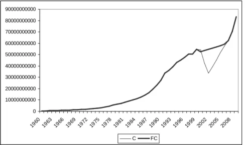
To deal with the Euro introduction and the associated changes of currency in circulation and sight deposits, we have used an exponential interpolation in the following way. First, we have
chosen some years before and after the drop of the series, that is, 1995 through 1999 and 2006. Second, by inspection of the data we decided that an exponential function would produce the best fit, and, thus, we used C = e(a + b t), where C denotes currency in circulation outside banks and t denotes time, where 1995=1, 1996=2, ..., 2006=12. Third, by using an OLS estimation procedure, we obtained,
Ln Ct = 24.5618109 + 0.01999468* t,
(896.6) (4.2)
where relevant t-statistics are given in parenthesis below the coefficients and diagnostic statistics are: Adj. R2 = 0.77, standard error = 0.0419. Taking natural logarithms, we calculated parameters a and b:
Ct = e24.5618 + 0.1999t.
Third, if the expression above is given, interpolation between 2000 and 2006 yields the results shown in Figure 2, where FC denotes forecasted C, which we used in equation (5) of the main text.
Figure 2: Actual and Forecasted Currency in Circulation (Spain 1960-2009)
0 10000000000 20000000000 30000000000 40000000000 50000000000 60000000000 70000000000 80000000000 90000000000 1960 1963 1966 1969 1972 1975 1978 1981 1984 1987 1990 1993 1996 1999 2002 2005 2008 C FC
C) Test Statistics
Figure 3a,b,c,d: CUSUM Test of Squares
a) Model 1 b) Model 2 -0.4 0.0 0.4 0.8 1.2 1.6 90 92 94 96 98 00 02 04 06 08 CUSUM of Squares 5% Significance -0.4 0.0 0.4 0.8 1.2 1.6 82 84 86 88 90 92 94 96 98 00 02 04 06 08 CUSUM of Squares 5% Significance c) Model 3 d) Model 4 -0.4 0.0 0.4 0.8 1.2 1.6 82 84 86 88 90 92 94 96 98 00 02 04 06 08 CUSUM of Squares 5% Significance -0.4 0.0 0.4 0.8 1.2 1.6 86 88 90 92 94 96 98 00 02 04 06 08 CUSUM of Squares 5% Significance