Welfare improving taxation on saving in a growth model

Department of Communication, University of Teramo

wpcom

unite.it ●

●

●

○○○

Welfare improving taxation on saving in a growth model

Xin Long

Alessandra Pelloni

Department of Communication Working Paper Series.

The Department of Communication Working Paper Series is devoted to disseminate works-in-progress reflecting the broad range of research activities of our department members or scholars contributing to them. It is aimed at multi-disciplinary topics of humanities, science and social science and is directed towards an audience that includes practitioners, policymakers, scholars, and students. The series aspires to contribute to the body of substantive and methodological knowledge concerning the above issues. Since much of the research is ongoing, the authors welcome comments from readers; we thus welcome feedback from readers and encourage them to convey comments and criticisms directly to the authors. Working papers are published electronically on our web site and are

available for free download (http://wp.comunite.it). Each working paper

remains the intellectual property of the author. It is our goal to preserve the author's ability to publish the work elsewhere. The paper may be a draft that the author would like to send to colleagues in order to solicit comments or feedback, or it may be a paper that the author has presented or plans to present at a conference or seminar, or one that the author(s) have submitted for publication to a journal but has not yet been accepted.

Welfare Improving Taxation on Saving in a

Growth Model.

Xin Long

IEOR Department, Columbia University

Alessandra Pelloni

Department of Economics, University of Rome "Tor Vergata"

March 2011

Abstract

We consider the optimal factor income taxation in a standard R&D model with technical change represented by an increase in the variety of intermediate goods. Redistributing the tax burden from labour to capital will increase the employment rate in equilibrium. This has opposite e¤ects on two distortions in the model, one due to monopoly power, the second to the incomplete appropriability of the bene…ts of inventions. Their relative momentum determines the sign of the welfare e¤ect. We show that, for parameter values consistent with available estimates, taxing capital more heavily than labour can be welfare increasing.

Keywords: Capital Income Taxes, R&D, Growth E¤ ect, Welfare E¤ ect.

JEL classi…cation: E62, H21, O41

1

Introduction

This paper examines how the tax burden should be distributed between capital income and labor income in a basic R&D model of endogenous growth. The standard optimal taxation results in a dynamic setting would imply that not taxing capital income is e¢ cient although it may not be desirable due to equity considerations. In this paper we show that in contrast to this conventional view, taxing labor income more heavily than capital income may also be ine¢ cient. The key feature of this economy driving this result is that pro…ts, from goods produced monopolistically and whose costly invention is the engine of growth in the model, are linearly increasing in employment.

Corresponding author: Faculty of Economics, University of Rome "Tor Vergata", Rome, Italy. Email: [email protected].

The conclusion that in the long run, capital income should not be taxed was …rst reached in Chamley(1986) and Judd (1985), and shown to be robust to the relaxation of a number of assumptions( see the overviews by Chari and Kehoe 1999 and Atkeson, Chari and Kehoe 1999). Jones et al.(1997) show that the conclusion holds for human as well as physical capital.

The literature on endogenous growth tends to reinforce the message that capital income should not be taxed, as doing so would have adverse e¤ects on the rate of growth which would compound over time( see the survey in Jones and Manuelli 2005)

We adopt for our analysis a standard R&D model of horizontal innovation, with an in…nitely lived representative agent, originally proposed by Rivera-Batiz and Romer (1991) and known as the "lab-equipment model". Given its ‡exi-bility and simplicity this model provides a tractable framework for analyzing a wide array of issues in economic growth.1 Entrepreneurs spend a …xed cost in order to develop new intermediate goods, over the production of which they then enjoy eternal monopoly power. Output in the …nal goods production sector is linear in the number of intermediate goods used so unbounded growth is possi-ble. There are two ine¢ ciencies in the model, one stemming from market power in the intermediate goods sector, one from the uncomplete appropriability of the social gains from innovating. We extend this benchmark model by introducing government spending and by explicitly analysing the decision to supply labour. Our main results concern equilibrium dynamics under the assumption that the government has no access to lump-sum taxes or public debt, holds constant the fraction of GDP allocated to public expenditure, and balances the budget at all times. The tax rates ( ie the labour income tax rate and interest income tax rate in our model) must adjust endogenously. Our exercise therefore focuses on the e¤ects of revenue-neutral changes in tax structure. Shifting the tax burden from capital to labour will increase employment and the productivity of each di¤erentiated product, whose demand is therefore increased. The production of each intermediate will then be more pro…table, and the distortion due to monopoly power lower. In the model, savings …nance the increase in the va-riety of products. This invention activity is more rewarding the greater their prospective demand. So a higher employment increases coeteris paribus the re-turn to saving and therefore linearly increases growth . However the increase in the tax on capital discourages savings and growth, thus worsening the dy-namic ine¢ ciency. A third distortion in the model is represented by goverment expenditure, which is assumed to be a constant fraction of GDP and to have no impact on consumers’utility or the productivity of the economy. Taxing both labour and capital income reduces this distortion. For reasonable parameter values the interplay between the various channels means that the optimal tax on capital is not only positive but very sizable and often higher than that on labour.

Studies based on R&D models similar to ours have generally found that

1_{See the excellent survey in Gancia and Zilibotti (2005) for a selection of the wide range}

taxing savings is detrimental to growth and welfare (e.g. Lin and Russo 1999 and 2002, Zeng and Zhang 2002). Zeng and Zhang (2007) study …scal issues adopting our same speci…cation of the horizontal innovation model but focus on a di¤erent issue, i.e. they compare the e¤ects of subsidizing R&D investment to the e¤ects of subsidizing …nal output or subsidizing the purchase of intermediate goods in terms of promoting growth. They consider distortionary taxation (i.e. taxes on labour income) but abstract from taxes on interest income.

This paper aims instead at further exploring the circumstances under which optimal factor taxation may involve a non-zero tax rate on capital income. A way in which taxing capital can be good is when government spending in-creases the marginal productivity of capital, as in Baier and Glomm (2001), Barro (1990), Barro and Sala-i-Martin (1992, 1995), Guo and Lansing (1999), Turnovsky (1996, 2000), Corsetti and Roubini (1996), and Chen (2007). The presence of an informal sector the income from which cannot be taxed or other restrictions on the taxation of factors are also grounds for the positive taxation of capital income (see Correia 1996 and Penalosa and Turnovsky 2005). Aiyagari (1995), Chamley (2001), Ho and Wang, (2007), Hubbard and Judd (1986) and Imrohoroglu (1998) have emphasized that if households face borrowing con-straints and/or are subject to uninsurable idiosyncratic income risk, so that excessive savings arise then the optimal tax system will in general include a pos-itive capital income tax. Asea and Turnovsky (1998) and Kenc (2004) …nd that increasing the tax rate on capital income may increase growth in a stochastic en-vironment. Conesa and Garriga (2003), Cremer et al. (2003), Hendricks (2003, 2004), Erosa and Gervais (2002), Song (2002), Uhlig and Yanagawa (1996) and Yakita (2003) show that in life cycle / OLG models the optimal capital income tax in general is di¤erent from zero. Conesa et al. (2008) quantitatively charac-terize the optimal capital income tax in an overlapping generations model with idiosyncratic, uninsurable income shocks and …nd the optimal capital income tax rate is signi…cantly positive at 36 percent. All these papers can be seen as examples of the argument in Judd (1999) that it is the presence of constraints (for the government or the individual) or suboptimal expenditure choices that makes capital income taxation desirable. Hence, they are second-best results.

All these arguments in favor of a positive rate of capital taxation are unre-lated to ours as we model a perfect foresight closed economy with in…nite lived agents no e¤ect of government expenditures on the rate of return of private factors and no human capital accumulation.

Two articles closer to our analysis are Pelloni and Waldmann (2000) and de Hek (2006). In the …rst paper a simple learning by doing model a la Romer (1986) is augmented by endogenous labour supply and it is shown that if the equilibrium is indeterminate capital taxation can increase growth and welfare. However, the scope of the result is limited because indeterminacy is only possible with a very high intertemporal elasticity of substitution in the model. de Hek (2006) studies the e¤ects of taxation on long-run growth in a two-sector endoge-nous growth model with physical capital as an input in the education sector and leisure as an argument in the utility function. If only capital income is taxed human capital accumulation will be encouraged and the long-run growth rate

may be increased. In order to isolate the labour employment factor from these considerations, in our model we do not introduce human capital accumulation. In Zhang et al (2008) the government should tax net capital income more heavily than labor income, however investment is subsidized at the same rate at which net capital income is taxed. We do not allow such subsidy.

A complete assessment of the welfare e¤ects of the tax program has to include an analysis of its e¤ect on the dynamic properties of the model. In fact it has recently been shown that factor taxes can a¤ect the stability properties.of the dynamic equilibrium and this possibility has to be taken into consideration. In particular, Ben-Gad(2003), Palivos et al. (2005), Raurich (2001) Schmitt-Grohe and Uribe (1997), among others have shown that the introduction of taxes and improductive government spending may make the equilibrium exhibit local indeterminacy. We show that this is not the case in this model, which features a unique unstable balanced growth

The rest of the paper is organized as follows: in section 2 the model is presented, in section 3 the general equilibrium conditions of the model are de-scribed, section 4 analyzes the labour supply e¤ect, the growth e¤ect and the welfare e¤ect of a capital income tax whose proceeds are used to subsidize labour. Finally section 5 does numerical calculations to show that even if the growth rate is decreased, such a tax can increase welfare for widely accepted es-timates of the relevant parameters and derives the optimal tax rates for various sets of parameters, section 6 concludes.

2

The Model

2.1

Households

We assume that in the economy there is a continuum of length one of identical households.2 _{Each has utilityU given by:}

U = Z 1 t=0 e t 1 1 C 1 _{h(H) dt (1)}

where C is consumption and H labour. is rate of time discount 1/ >0 is the intertemporal elasticity of substitution. The following conditions ensure non satiation of consumption and leisure: >0and:

h(H)>0 (2)

(1 )h0(H)<0. (3)

Strict concavity of instantaneous felicity imposes:

(1 )h00(H)<0 (4)

2_{As Zeng and Zhang (2007) note, normalizing the population to unity removes from the}

and

h00_h

( 1) h

02_{>0. (5)}

The instantaneous budget constraint consumers face is given by:

_

F =r(1 l_k)F+ n(1 kl)N+w(1 tw)H C. (6)

Households derive their income by loaning entrepreneurs their …nancial wealth

F (of which all have the same initial endowment), by pro…ts n(net of the interest payments) of the N …rms and by supplying labourH to …rms, taking the interest rate r and the wage rate w as given. Capital income is taxed at the rate l

k while labour income is taxed at the rate tw. Optimization at an interior point implies that the marginal rate of substitution between leisure and consumption equals their relative price:

h0

h =

w(1 tw)( 1)

C . (7)

Optimal consumption and leisure must also obey the intertemporal condi-tion: _ C C + h0 hH_ = _ = r(1 l_k) (8)

where is the shadow value of wealth. Given a no Ponzi game condition the transversality condition imposes:

lim

t!1 Fexp( t) = 0. (9)

2.2

Firms

In this economy there are a …nal goods sector and an intermediate goods sector. The former is perfectly competitive, whereas the latter is monopolistic. R&D activity leads to an expanding variety of intermediate goods. All patents have an in…nitely economic life, that is, we assume no obsolescence of any type of intermediate goods.

The production function of …rmiin the …nal goods sector is given by:

Y(i) =AL(i)1

Z N

0

x(i; j) di (10)

whereY(i)is the amount of …nal goods produced andL(i)is labour used by …rm

iandx(i; j)is the quantity this …rm uses of the intermediate goods indexed by

j. For tractability bothiandj are treated as continuous variables. We assume

0< <1. The …nal goods sector is competitive and we assume a continuum of length one of identical …rms. We can then suppress the index i to avoid notational clutter. Firms maximize pro…ts given by

Y wL

Z N

0

wherewis the wage rate and P(j)is the price of the intermediate goodj. By pro…t maximization, the demand for goodj is given by:

x(j) =L A P(j)

1 1

(12) and labour demand by:

w= (1 )Y

L. (13)

Since the …rms in the …nal goods sector are competitive and there are constant returns to scale their pro…ts are zero in equilibrium. In contrast the …rms which produce intermediate goods with patent which they invent then earn monopoly pro…ts for ever. The cost of production of the intermediate goodj, once it has been invented, is given by one unit of the …nal good.

The present discounted value at timet of monopoly pro…ts for …rm j, or in other words the value of the patent for thejth_{intermediate goodV(j; t)at time}

tis: V(j; t) = 1 Z t (P(j) 1)x(j)e r(s;t)(s t)ds (14) wherer(s; t)is the average interest rate during the period of time from tto s. The inventor of thejth _{intermediate good choosesP(j)to maximize (P(j)}

1)x(j) where x(j) is given by 12, so for each j, the equilibrium price is and quantity are: P(j) =P = 1 (15) and x(j) =x=LA11 2 1 _{. (16)}

The price is higher than the marginal cost of producing good j, and the quantity produced, x(j); is therefore lower than the socially optimal level. This is in fact the …rst ine¢ ciency in the model, a straitforward consequence of market power in the intermediate sector. Notice a higher labour supply implies a higher quantity of each intermediate goods in equilibrium. So a tax program leading to increasing L can increase welfare by reducing the ine¢ ciency due to monopolistic conditions.

Plugging equation 16 in equation 10 gives us equation

Y =N LA11 2

1 (17)

while plugging 17 in 13 we have:

w=N(1 )A11 2

1 . (18)

Notice pro…ts are given by a consequence of 16 and 15:

The cost of development of new products is and there is free entry in the market for inventions. Intermediate goods …rms will push the price of a patent to equate its cost. Here a second ine¢ ciency in the model appears, which is due to an appropriability problem: only the discounted value pro…ts as opposed to all of social surplus originating from an invention, is taken into account when deciding whether to pay for research. This means that the pace of invention will be too low.

If we drop the j index in V, 14 can be written as the Hamilton Jacobi Bellman equation: r= V + : V V (20)

which allows us to interpret it from an asset pricing perspective. The return on holding a blueprint, rV, is given by dividends ; plus the capital gains, ie the change in its value V. Later we show that, in a growing economy, we must have V= in equilibrium at all times. But if V= at all times; 20, given 19, implies that in equilibrium we will have:

r=C1L (21)

where: C1 1A

1 1

1+

1 (1 ). 3 Notice that the higher is labour supply the

higher is the interest rate. As the sales of each intermediate good and therefore pro…ts are increasing in labour supply, for their present discounted value to be equal to the given cost of an invention, the interest rate will have to increase.

2.3

Government

We assume government consumption G equals a …xed fraction, g, of output: G=gY. We rule out a market for government bonds and assume that the gov-ernment runs a balanced budget. The revenue from income taxes is used for …nancing expenditures. In equilibrium:

r l_kF+twwL=gY (22)

where on the left-hand side we have in‡ows and on the right-hand side we have out‡ows.

3

Market Equilibrium

In calculating the equilibrium in the …nal goods market, intermediate goods used in production,xN;are subtracted from …nal productionY to obtain total value added. All investment in the model is investment in research and devel-opment of new intermediate goods N_. The economy wide resource constraint is therefore given by:

3_{It also means}

Y xN=C+ N_ +gY (23) We are now ready for the following:

De…nition 1 In a competitive equilibrium individual and aggregate variables are the same and prices and quantities are consistent with the (private) ef-…ciency conditions for the households 6, 7, 8 and 9, the pro…t maximization conditions for …rms in the …nal goods sector, 12 and 13 (or 18), and for …rms in the intermediate goods sector, 15 (or 16) and 21, with the government budget constraint 22 and with the market clearing conditions for labour (H =L), for wealth (F =V N), and for the …nal good, 23.

The following relationship between before-tax labour income and before-tax capital income holds in equilibrium:

wL=rF = 1 (24)

From 22 and 24 we can then infer that:

tw=

g

1

l

k (25)

In the appendix, we show that, if the economy is to grow at any time, V will have to be equal to at all times. Given this from the de…nition of equilibrium we can now arrive at the following:

Proposition 2 The competitive equilibrium conditions in the model give rise to the following di¤ erential equation for labour:

_ L= B(L) A(L) (26) where A(L) h00 h0 + h0 h(1 ) (27) and B(L) C1 h((1 ) h0 1 + l k g (1 ) + C1L 1 l k 1 g (1 ) (28) :

Proof. See Appendix 1

If a balanced growth path (hence BGP) exists, variables grow at a constant rate along this path, and in particular employment is constant at a value Le. Given 26 we have:

Proposition 3 The condition for the existence of a BGP equilibrium in this model is that 26 has a …xed point Le between 0 and 1, implicitly de…ned by B(Le) = 0;consistent with the TVC and with a positive growth rate for capital and consumption given by:

=C1Le(1

l

k) _{. (29)}

Proof. From 61, in a BGP, ie whenL_ = 0;C and N will grow at the same rate. From 8 this is seen to be given by 29

Speci…c restrictions on parameters ensuring existence of a BGP equilibrium will be considered after introducing a speci…c functional form for the function h. However for the general case we can establish some interesting results on the uniqueness and stability of the BGP, assuming existence.

If we write B(L) m(L)-f(L), wherem(L) C1h((1h0 ) 1 + lk g

(1 ) and

f(L) +C1L

h

1 l_k 1 ₍₁g ₎ i;BGP employmentLeis the point of intersection between the two curves m and f, both continuous and di¤eren-tiable. Below we will see that if > 1 or if < 1 and tw 1 (1 ), B’(Le)>0, ie whenever the two curves intersect the m(L) curve crosses the f(L) curve from below. But of course a continuous function cannot cross another continuous function from below twice in a row. This establishes uniqueness of equilibrium given its existence, under the restrictions > 1;or <1 and -tw (1 ) 1.

We say that the equilibrium is locally indeterminate when there is a con-tinuum of equilibrium paths that converge to the same balanced growth path. Agents can coordinate on any equilibrium within such a continuum of equilib-ria. Each of these equilibria exhibits di¤erent growth rates during the transi-tion. Therefore, local indeterminacy of equilibria may explain divergences in short-run growth rates among countries with similar fundamentals. Moreover, sunspot equilibria may arise when the equilibrium exhibits indeterminacy and, thus, economic instability may be induced by shocks that do not a¤ect the fundamentals.

In this model, the discussion of the stability of equilibrium is closely related to that of uniquess.

A(L) is always strictly positive for all values ofL, by the negative de…niteness condition of the hessian of the utility function 4, so the di¤erential equation 26 is de…ned for all values ofL beween 0 and 1. To study the dynamic nature of a …xed point of 26, i.e. of BGP labour supply, we have to sign dL_(Le)=dL:e If this derivative is positive the …xed pointLe is a repeller and the BGP is locally determinate. If dL_(Le)=dLe is negative then Le is an attractor, ie there is local indeterminacy. We have: dL_ dL( ~L) = B0_{( ~L)} A( ~L) A0_{( ~L)B( ~L)} A2_{( ~L)} = B0_{( ~L)} A( ~L) (sinceB( ~L) = 0).

But as said above and proved belowB( ~L) = 0impliesB0_{( ~L)>0 if >1;or if} <1andtw 1 (1 ). So in these cases the equilibrium will be unique and unstable and the economy will always be on the BGP.

Proposition 4 If a BGP equilibrium de…ned by B( ~L) = 0exists, while either

> 1, or < 1 and tw 1 (1 ) are true, then B( ~L) > 0 ie the

BGP equilibrium is unique and locally determinate, so there is no transitional dynamics to it.

Proof. See Appendix

As the necessary conditions for B’(L) negative require unrealistic parameters’ values (in particular a very low or a very hightw);from now on we concentrate on the case of a determinate and unique BGP equilibrium.

4

E¤ects of Taxes

4.1

E¤ect on labour

It is relatively simple to calculate the e¤ect of taxes on employment in this model because the wage rate does not vary with it. As said above equilibrium labour supply can be expressed as the solution to B( ~L) = 0. The e¤ect of shifting the tax burden from labour to capital can be deduced by using the total derivative ofB( ~L) = 0with respect to labour and the tax ( l

k);keeping the ratio of government expenditureg …xed. This gives us:

dL~ d l k = C1 (_h01)h L~ B0_{( ~L)} : (30)

With B0( ~L) > 0, the case on which we focus, this derivative signs as the numerator of the fraction. To sign this, in the appendix we show that the TVC can be rewritten as

~

L < ( 1)h

h0 . (31)

This is, in light of ??, the well known condition that consumption must be higher than labour income For >1, we can easily see that we will always have

dL~ d l k

>0. We are therefore ready to state the following:

Proposition 5 An increase in the tax rate on capital income whose proceeds are used to reduce the tax on labour income will increase employment in equilibrium if and only if (_h01)h >L;~ given determinacy. This condition is always satis…ed if >1.

If h’>0, ie >1;UcL>0; ieleisure and consumption are substitutes, so that taxing capital making consumption more attractive makes leisure less attractive, helping to o¤set the labour-leisure distortion due to labour income taxation. We also notice that the Frisch ( compensated) elasticity of substitutionEf;given our utility function, is given by:

"F =

1

L(h_h”0 + 1 1 h 1h0)

For convex preferences, h_h”0 >0;while 1 1 h 1h0<0;so this elasticity will be

bigger the higher is_j 1 1 h 1_h0_{j , ie, coeteris paribus, the higher is :}

4.2

E¤ect on Growth

The growth e¤ect of tax l k is: d d l k = @ @rr 0_{( ~L)}dL~ d l k + @ @ l k = r (1 l k) l k l kdL~ ~ Ld l k 1 ! .

Not surprisingly the condition for the tax change to be growth increasing is stricter than the condition for it to be employment increasing, because for growth to increase we need the net interest rate to increase not just the gross interest rate, which is a linear function of the employment rate. When l_k >0, the condition for the policy to be growth increasing is that the elasticity of labour supply with respect to the tax _ddL=~l L~

k= l k

is not only positive but bigger than l_k=(1 l_k). In particular we have:

Proposition 6 An increase in the tax rate on capital income whose proceeds are used to reduce the tax on labour income will increase growth in equilibrium, given determinacy, if and only if

( 1)h h0_L~ 1 1 l k 1 1 + l_k g 1 1 + (1 ) 1 hh00 (h0₎2 >0: (33)

This condition requires > 1 tw (1 l_k)

2

and, regardless of the level of tw;is

never satis…ed if 1

g

1 2 _. Proof. See appendix.

Intuitively, the negative e¤ect of the tax on growth, for a given gross of tax interest rate, will be lower the higher is ;through the Euler equation. Moreover, as we have seen before, the Frisch elasticity of labour supply is increasing in ;so the tax will provoke a stronger positive e¤ect on employment and the gross of tax interest rate.

4.3

E¤ect on Welfare

Given , the BGP rate of growth, andLe the BGP labour supply, it is possible to calculate maximum lifetime utilityV along a balanced growth path:

V = Z 1 t=0 e [ (1 )]t 1 1 C(0) 1 _{h( ~L) dt. (34)}

In Appendix 2 it is shown how to express V as a di¤erentiable function of l

k and L~ (itself a function of lk). The e¤ect on welfare of an increase in the tax rate l

k is then positive if ddVl k

is positive. To simplify calculations, we consider the following monotonically increasing transformation ofV: log[(1₁ )V]. d(log[(1 )V])

(1 )d l

k signs as

dV d l

k but is easier to manipulate algebraically so we will

use it. We have:

d(log[(1 )V]) (1 )d l k = @(log[(1 )V]) (1 )@ l k + dL~ d l k @(log[(1 )V]) (1 )@L~ (35)

In Appendix 2 we also show the following:

@(log[(1 )V]) (1 )@L~ = h0 h _L~ 1 ( 1) ₍hh_h0₎002 1 + 1 ( 1)h h0_L~ 1 (36) and @(log[(1 )V]) (1 )@ l k = 1 1 1 + l k g 1 . (37)

Substituting 30, 36 and 37 in 35, we get:

d(log[(1 )V]) (1 )d l k = (1 l k) ( 1)h h0L~ 1 (1+ lk g 1 ) (1 ) 1 hh 00 (h0)2 +1 ( 1)h h0L~ 1 + l k g 1 ( 1)h h0_L~ 1 B0_{( ~L)} C1 . (38) Notice the denominator is always positive by1 + l

k 1g > 0 and 31 and

withB0( ~L)>0. Hence we arrive at the following:

Proposition 7 IfB0_{( ~L)>0;ie if the BGP equilibrium is determinate, the}

suf-…cient and necessary condition for an increase in the tax rate on capital income whose revenue is used to reduce the tax on labour income to improve welfare is:

(1 l_k) ( 1)h h0_L~ 1 1 + l k g 1 ( 1)h h0_L~ 1 + (1 ) 1 hh00 (h0₎2 0 (39) Of course, if a value for l_kexist such that for this value 39 holds as an equal-ity, while it holds strictly for lower tax rates, 39 gives us an implicit expression for the optimal tax rate, given the tax program.4

In the appendix we prove the following:

Proposition 8 If > 1, or 0 < < 1 and ( 1)h

h0_L~ > 1;it is possible for a

revenue neutral increase in the tax rate on capital income to increase welfare while decreasing growth .

4_{This way of solving the Ramsey problem ie by chosing the instrumental variables ( here}

the tax rates) by optimizing the indirect utility function, which is derived in the private agent’s reaction from a decentralized economy is known as the dual formulation.

This result goes against the widely held belief, that when growth is subopti-mal, further decreasing it cannot possibly be a Pareto improvement, no matter what static gains it could allow, as the growth e¤ects compound over time. However, in the next section we will show that this surprising …nding is more than a theoretical possibility and that for speci…cations of tastes and technology parameters often used in calibration exercises it is possible for the tax program to induce Pareto improvements but reduce growth. The example we o¤er are also useful for a better interpretation of the mechanisms at work in producing the results.

4.4

A Parametric Example

We consider here the following class of functions for the disutility of labor:

h(L) = (1 L)1 (40)

where >1 if >1 or <1< + if0< <1.

First we notice that by plugging 40 and its derivative in 26 withB( ~L) = 0

we obtain the following value for employment in equilibrium ( also using 30):

~ L= (1 tw) 1 1 C1 (1 tw) + ₁2+ ( 1) 1 l_k (41) To be more precise, L~ as de…ned in 41, will be equal to employment in a BGP equilibrium if it is less than 1 and if it is consistent with positive growth and with the TVC.

Proposition 9 Conditions for the existence of a determinate equilibrium with positive growth are :

(1 tw) + (1 ) 1 lk < _C 1 < 1 1(1 lk) + 2 1 + (1 l_k) (1 tw) (42)

With >1;these conditions are su¢ cient as well as necessary, and in fact the …rst, as well as the TVC, will always hold. With < 1 a further condition ( derived from the TVC) is:

C1 > (1 ) 2 1 l k 2 (43)

Finally, the necessary and su¢ cient condition for determinacy is:

tw<1

(1 )(1 l

k) ( 1)

( + 2) (44)

Reverting all these inequalities we have necessary and su¢ cient conditions for an indeterminate BGP equilibrium with positive growth.

Proof. With h given by 40, we have from 63: B_C0(L) 1 = 1 + l k g 1 + 2 1 + ( 1) 1 l

k :Notice this is just the denominator of the fraction on the

left-hand side of 41. So under determinacy ie whenB₀( ~L)>0 (which gives us 44);

this denominator is positive. GivenB₀( ~L) >0; the …rst inequality in 42 must hold forL~ to respect its upper bound ie to be smaller than one, as can be easily seen from 41. Notice this condition is always true for >1:For positive growth we also need the net interest rate to be bigger than the rate of time discount or

C1(1 l

k) ~L > by 29:Just by using 41 when the denominator of the fraction in

41 is positive(ie under determinacy) this condition gives us the second inequality in 42. Finally the TVC that (1 ) <0is always true for 0with >1:

With <1;by using 29 to express in terms of andL~ and using 41, assuming determinacy, the TVC can be found to impose 43. The proof of the statement on the indeterminate equilibrium is obtained proceding in a strictly analogous way but noticing that the denominator of the fraction on the left-hand side of 41 is negative with indeterminacy.

We add that if 44 holds, then

1 1(1 l k) + 2 1 + (1 l_k) (1 tw) > (1 ) 2₍₁ l_k) 2 ;so it is possible

for both the second inequality in 42 and the inequality in 43 to hold. With indeterminacy 1 1(1 l k) + 2 1 + (1 lk) (1 tw) < (1 ) 2₍₁ l_k)

2 so again the inverses of the

second inequality in 42 and of the inequality in 43 will not be inconsistent. By 29 and 41 the BGP growth rate is:

= C1 1₁ 1 + lk g 1 (1 l k) 1 + g 1 + 1 + l k g 1 1 1 1 + + (1 + l k) 11 (1 lk) . (45) while using 41 the e¤ect of l

k on BGP labour supply can be seen to be:

dL~ d l k = 1 +1 g 1 ( 1)2 1 +C1 1 + ( 1) 1 h 1 ₁g + ₁2 + 1 + l k 1 + ( 1) 1 i2,

as we already now from the general case the e¤ect on labour will be always positive for >1:

By Proposition 7 a positive welfare e¤ect givenB0_{( ~L)>0;requires:} 1 1 1 L~ ~ L 1 ! (1 l_k) 1 + l_k g 1 ( + 2) ~L ( 1)(1 L~) 0 (46)

To calculate the optimal asset income tax we plug in 46 the expression for

Lgiven by 41 and we equate it to zero:5

h ( 1)2₍₁ l k) +C1( + 2) i (1 l k) 1 + l k g 1 ( 1) ( 1) C1 = ( + 2) 1+ l k 1g ( 1) C1 ( 1) +( 1)(1 l k)+C1 1+ l k g 1 . (47)

The root of this non linear equation in l

k gives us the optimal value of the tax, for each six-tuple of parameters_f ; ; g; ; ; C1g:For all the parameterizations

we consider, the expression is always decreasing in l_k for 0 l_k 1, so the stationary point of the welfare function we thus …nd corresponds to a maximum.

4.4.1 Calibration

Now we use 47 to calculate the optimal tax rates for reasonable values of the parameters.

Our simulations start from setting values for the the 7-tuplenr; ;L; ; ; g;~ l_k0o

, where l

k0 stands for the initial capital income tax rate. These values imply

values for (through 29), for tw (through 25), for (through 41 and using

C1 =r=L by 21). We then solve 47 for lk, given the values so obtained for

f ; ; g; ; ; C1g:

Our choices in feeding numbers to the model follow related studies of nu-merical R&D models (e.g. Jones and Williams 2000, Strulik 2007 and Zeng and Zhang 2007).

For the intertemporal elasticity of substitution, we follow a general consensus for it to be close to 0.5 and therefore set = 2, as our benchmark ( see Hall 2009).

The time preference parameter is usually thought to belong to the interval 0.01-0.05. As Strulik (2007) we set the benchmark value at 0.02 and let it vary from 0.01 to 0.03.

A range of values for labour supply are used in calibration exercises. For example Jones et al. (2005) useL~ = 0:17while a value of 0.3 is often adopted. In 2005 the average US worker used 21 percent (24 percent) of her (his) time endowment to work.6 _{We choose 0.23 as our benchmark value and 0.17-0.3 as} our range for sensitivity analysis .

Coming to 1= , which is the price markup in our model, we choose for it the range (1.1, 1.37) and take 1.2 as the benchmark. We thus follow Jones and Williams (2000) who make the markup vary between 1.05 and 1.37, and Strulik (2007) who …xes it at 1.27_.

6_{Source: US Bureau of Labor Statistics, current Population Survey, March 2005. For}

further discussion see chapter 2 of Borjas (2009).

7_{Jones and Willians note that in Romer (1990) the monopoly markup is equal to the}

inverse of the capital share1= . Empirically, this implies a gross markup (the ratio of price to marginal cost) of approximately 3, sharply exceeding empirical estimates of 1.05 to 1.4. In our model the capital share is =(1 + ), so the trade o¤ between matching income shares and matching markups is less severe. Taking the data from the IMF’s World Economic Outlook (April 2007) and the European Commission’s Employment in Europe (2007), in the

The long-run growth rate, the values used in related researches include 1.25 percent (Jones and Williams 2000), 1.75 percent (Strulik 2007), and 3 percent (Zeng and Zhang 2007): in what follows we check that the equilibrium growth rate generated in our model falls within these bounds.

Again following Jones and Williams (2000), the benchmark for the steady-state interest rate is set to 7.0 percent, which represents the average real return on the stock market over the last century in the US, and let it vary between 4.0 percent and 10.0 percent.

Turnovsky (2000) uses 14 percent for the ratio of non productive government expenditure to GDP while Gomez (2007) uses the government consumption to GDP ratio at 13.9 percent. We set as benchmark forgthe value 14 percent and consider the interval (0.08,0.18) as a robustness check

Gouveia and Strauss(1994) estimate the parameter that best approximates the average income tax rate under the actual US income tax system to be 0.258. We then choose as our benchmark value for l_k0 0.26 (also adopted by Conesa et al. 2009).

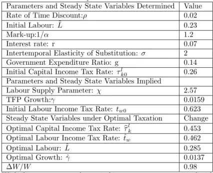
Our choices and results as regards the baseline economy are summarized in Table 1:

Table 1: Baseline Economy: Parameterization and Results. Parameters and Steady State Variables Determined Value

Rate of Time Discount: 0.02

Initial Labour: L~ 0.23

Mark-up:1= 1.2

Interest rate: r 0.07

Intertemporal Elasticity of Substitution: 2 Government Expenditure Ratio: g 0.14 Initial Capital Income Tax Rate: l

k0 0.26

Parameters and Steady State Variables Implied

Labour Supply Parameter: 2.57

TFP Growth: 0.0159

Initial Labour Income Tax Rate: tw0 0.623

Steady State Variables under Optimal Taxation Change Optimal Capital Income Tax Rate: _bl_k 0.453 Optimal Labour Income Tax Rate: ^tw 0.462

Optimal Labour: L^ 0.285

Optimal Growth: ^ 0.0137

W=W 0.98

With these parameters the capital income tax rate associated with maximum utility_bl_k is 45.32 percent while the labour income tax rate drops from 62.33 percent to 46.23 percent.

US capital share of income is 39.7% (2005), in EU-15 it is 41.2% (2006) (among which the highjest is in Spain, at 45.5%). With markup1:2, =(1 + ) = 0:4545; with markup 1.37 it is

This is striking because the tax rate on savings is not only positive but very close in value to the tax rate on labour income.

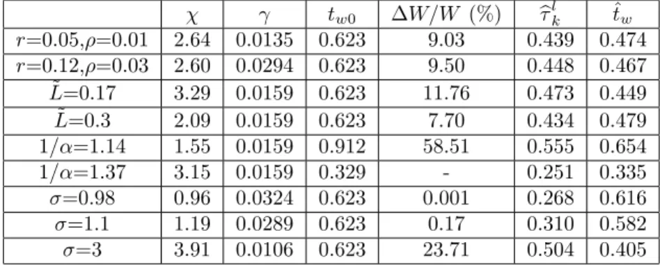
Now we adjust the values of the variables n ; ; r; ;L~o so to check the robustness of our result and to from a better picture of the e¤ects at work. The parameter-couple(r; )need vary in the same direction, i.e., higher interest rate has to be accompanied by a higher time discount factor to generate a plausible . Alsotw0has to change when changes, through 30. Finally a di¤erent value

of is now implied by the baselineL~ ( by 41), as we report in column 2. Table 2: Alternative Parameterizations

tw0 W=W (%) blk t^w r=0.05, =0.01 2.64 0.0135 0.623 9.03 0.439 0.474 r=0.12, =0.03 2.60 0.0294 0.623 9.50 0.448 0.467 ~ L=0.17 3.29 0.0159 0.623 11.76 0.473 0.449 ~ L=0.3 2.09 0.0159 0.623 7.70 0.434 0.479 1= =1.14 1.55 0.0159 0.912 58.51 0.555 0.654 1= =1.37 3.15 0.0159 0.329 - 0.251 0.335 =0.98 0.96 0.0324 0.623 0.001 0.268 0.616 =1.1 1.19 0.0289 0.623 0.17 0.310 0.582 =3 3.91 0.0106 0.623 23.71 0.504 0.405 In all cases but one the e¤ect of raising the capital tax above the initial rate is welfare increasing, though growth decreases. The only exception is when

1= =1.37, when the optimal tax rate on capital is 0.251. In order to check that the parameter values for are reasonable, we calculate the corresponding compensated elasticity of labour supply (or, the Frisch elasticity of labour sup-ply, which is obtained by keeping constant the shadow value of wealth) and we compare our results with the available estimates. With the speci…cation of h in 40, given 32, the Frisch elasticity of labour supply in BGP is given by

"F = 1 +

1 11 L

L

so it is decreasing in ;increasing in and decreasing in L. Most of the values for

"F;implied by our calibrations, when the optimal tax structure is implemented in our model are between 1 to 2, with 3.67 the highest (with =0.95) and 1.09 the lowest (with =4). In the benchmark parametric space, the Frisch elasticity is 1.59 when the optimal tax structure is used. These values are broadly consistent with recent estimates found in the literature, which range from 0.5 to 3 or higher (see, for example, Domeij and Flodén 2006; Imai and Keane 2004; Prescott 2006, Rogerson and Wallenius 2009, Shimer 2008), even if the micro-elasticities are much lower. Economy-wide permanent changes in taxes are in fact more likely to be associated with large responses in labour supply as they induce coordinated changes in work patterns, while frictions can attenuate short-run margin elasticities substantially ( see Chetty et al. 2009). 8

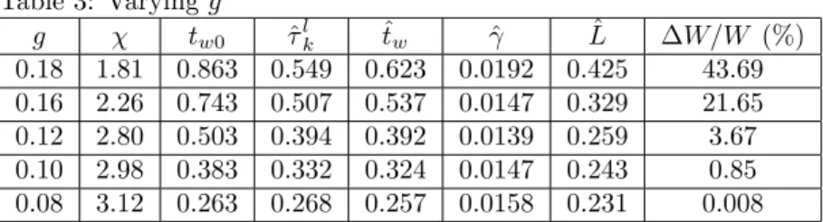
In table 3 we report separately on results for di¤erent values of g, with the other parameters kept at their benchmark values: of course a higher level of g, implies a higher level of tw0;through 30, and so if we want to keep initial L

constant has to vary as well. Table 3: Varyingg g tw0 ^lk t^w ^ L^ W=W (%) 0.18 1.81 0.863 0.549 0.623 0.0192 0.425 43.69 0.16 2.26 0.743 0.507 0.537 0.0147 0.329 21.65 0.12 2.80 0.503 0.394 0.392 0.0139 0.259 3.67 0.10 2.98 0.383 0.332 0.324 0.0147 0.243 0.85 0.08 3.12 0.263 0.268 0.257 0.0158 0.231 0.008

4.5

Comparison between the market economy and the

so-cial planner’s economy

In this subsection we compare the social planner’s equilibrium with the market equilibrium. Our main aim is to rule out that our result on welfare being improved while the growth rate is reduced is due to the fact that the BGP growth rate in the market economy is higher than the social optimum.

Variables keep the same meaning as in the market economy, but the index s is used to show they characterize the social optimum. LetXs R₀NsXs(i)di, whereXs(i)is the amount of each type of the intermediate goods in the social planner’s economy andXs is the total amount produced of such goods. Then the …nal output in equilibrium can be expressed as

Y =AL1_s

Z Ns 0

Xs(i) di. (48)

The Hamiltonian for the social planner’s problem is:

J = C 1 s 1 h(Ls)e t_{+ A(1 g)L}1 s Z Ns 0 Xs(i) di Cs Z Ns 0 Xs(i)di ! (49) where is the Lagrangian multiplier attached to the social budget constraint. The social planner decides on the optimal path of the control variableLs, Cs, andXs(i), and that of the state variableNs. The key optimality conditions are:

Xs(i) = (A(1 g)) 1 1 11 _L s; (50) Cs= ( 1)h(Ls) h0_(Ls) (A(1 g)) 1 1 1 (1 )N s; (51)

_ Cs Cs +h0(Ls) h(Ls) _ Ls = _ = 1 (A(1 g))11 1 _L s. (52) In the balanced growth path,Ls is constant soL_s= 0. From 52 we get

_ Cs Cs = 1 _{(A(1 g))}11 1 _L s . (53)

In equilibrium, the rate of return used by the social plannerrs is then:

rs=

1

(A(1 g))11 1 L

s. (54)

Substituting 50 into 48 we get

Ys=A

1

1 1 _L

sNs (55)

By using the equations 50, 53 and 55 and the fact that the investment I

equals N_s, the resource constraint can be expressed as

_ Ns Ns = 1 Ns (Ys(1 g) Cs Xs) = 1 (A(1 g))11 1 _L s 1 ( 1)h(Ls) h0_(Ls)Ls . (56) We use s to denote the BGP growth rate in the centralized economy. In the BGP, _ Cs Cs = N_s Ns = _s.

The transversality condition requires 0 < _s < rs, which, from 54 and 56 is equivalent to:

0< ( 1)h(Ls)

h0_(Ls)Ls <1. (57)

This is di¤erent from the analogous condition 31 in the market equilibrium. We exploit this di¤erence to compare the steady state labor supply in the social planner’s economy and that in the decentralized economy. Given our speci-…cation of the utility function, (_h0₍1)_Lh₎(_LL) equals 1₁1_LL, which is a strictly

decreasing function of L. But then 1₁1 Ls

Ls < 1 < 1 1

1 L

L (by 31 and 57) we deduce that the steady state labor supply in the social planner’s economy is larger than in the market economy.

For optimal growth to be lower than initial growth in the market economy we would need C1L(1- kl)> rs;and a fortiori, since Ls > L; 1A

1 1 1+ 1 ₍₁ )(1 kl)> 1 (A(1 g)) 1 1 1 _or kl <1 1 g 1 1 :For realistic and g this would require a negative kl:

4.5.1 Interpretation of results

We are now ready to further comment on our …ndings that given observed levels of consumption government spending, a tax rate on capital as high as 26 percent, should not only not be reduced to zero, but generally raised to reduce the tax burden on labor.

In fact, in most of the cases we consider the optimal tax rate on assets is generally (much) higher than 26 percent and in fact very often higher than the optimal tax rate on labour. In particular l

k is increasing in ;decreasing in L, and decreasing in the mark up, while both tax rates are increasing in g, with the tax rate on asset income higher than the one on labour income, but for very high levels of g.

To interpret these results, consider that on …rst impact, the shift of the tax burden from capital to labour does not in‡uence the consumers’disposable income but increases the opportunity cost of leisure. Since the income e¤ect is zero, the increasing wage only has a substitution e¤ect on leisure, which causes labor supply to increase. Further, the increased labor supply induces a higher demand for the intermediate goods. This in turn induces a higher demand for investment in R&D so the interest rate will rise. But the after-tax interest rate is still smaller than the interest rate in a no-tax economy. Since the BGP growth rate is a monotonically increasing function of the after-tax interest rate, it also decreases.

There is a positive spillover from labour in the economy, linked to the pres-ence of market power by …rms. Firstly, increased labor supply causes a positive spillover as it increases pro…ts and the value of patents. The worker considers only the increase inw but output increases by w1

1+ where

1

1+ is the income

share of labor. The di¤erence is a spillover. Notice the size of this spillover is positively related with the value of . This helps us to understand why the pro-gram which increases equilibrium employment is particularly bene…cial when is high. This spillover occurs because the price of intermediate goods is greater than their marginal cost so increased demand for an intermediate good has a …rst order bene…t for its inventor. Secondly, the introduction of a new inter-mediate good causes increased welfare because it causes increased wages. The inventor only considers the part of the contribution to production that goes to capital (here income on patents). So the e¤ect of an invention on the present discounted value of income is the cost of inventing divided by the income share of capital, that is

1+ . When the return to capital is decreased after the increase

in the capital income tax and the parallel decrease in the labour income tax, the pace of invention of new patents will be slowed down. So this is a negative spillover, worsening the dynamic ine¢ ciency in the model. The optimal tax policy depends on the relative strength of the distortions.

The tax rate on capital will be higher the higher is the Frisch elasticity of labour supply. As this elasticity is positively related to ; a higher value of makes the bene…cial e¤ects of taxing capital more likely.The Frisch elasticity also depends negatively onL~ ( and on ;which is however an implied parameter

in our calibration so we do not comment on its e¤ect): a smallerL~ means that a small decrease of the tax rate on labour income will cause labour supply to increase much, thus making for a bigger reduction in the monopoly distortion and a relatively less important worsening of the appropriability failure.

Moreover for a given e¤ect of the tax program on the net interest rate, the higher is the lower will be the e¤ect on the growth rate and the less important the worsening of the dynamic ine¢ ciency. A bigger means lower intertemporal substitution elasticity of consumption, or that consumers weigh more the current consumption (lower) than the future (higher) ones. So, when the instantaneous consumption is increased along with employment this increment is given more weight than the future loss in consumption.

Finally, with higher subjective discount rate , although consumption will grow at a lower rate with a higher tax on capital, this dynamic loss is discounted more heavily and thus the overall welfare e¤ect is more likely to be be positive.

5

Conclusions

This study adds value to the literature on non-zero optimal capital income tax-ation. We show that raising taxes on savings above 26 percent and reducing taxes on labour income correspondingly to …nance government expenditures, can be welfare improving in a model of endogenous technological progress. This can happen because in the model there are two ine¢ ciencies, one related to the market power of …rms, the second related to the appropriability problem related to the invention of new products. The tax program has opposite e¤ects on the two distortions. The increase in the interest income tax and correspond-ing decrease in the labour income tax changes the opportunity cost of leisure without any change to disposable income, so labour supply will increase due to the substitution e¤ect. Raising labour supply increases the quantity of goods produced by monopolistic …rms so that the welfare cost of monopoly is reduced. The after-tax interest rate is reduced and so the growth rate goes down, ie the second distortion(which provokes an ine¢ ciently low rate of growth even before the change in the tax structure) is worsened. We have shown that a positive e¤ect of capital income taxation is more likely the higher the elasticity of labour supply, the lower the elasticity of intertemporal substitution in consumption and the lower the income share of labour.

Our result shows that the sign of the growth e¤ect of a tax program is not necessarily the same as that of the welfare e¤ect and that they should be analysed separatedly, even in models when growth is sub-optimal.

In future research we plan to explore the generality of the result along two main directions: ie considering a richer tax structure, including consumption taxes and considering a model of vertical rather than horizontal innovation. Further developments would be considering home production and the depen-dence of the marginal utility of leisure by its economy-wide average level.

References

[1] Alesina, A., E. Glaeser, and B. Sacerdote 2005. Work And Leisure In The US And Europe: Why So Di¤erent?, NBER Macroeconomic Annual 2005. [2] Aiyagari R. 1995. Optimal Capital Income Taxation with Incomplete Mar-kets, Borrowing Constraints, and Constant Discounting. Journal of Political Economy 103(6), 1158-75, December.

[3] Asea P. and Turnovsky S. 1998. Capital Income Taxation and Risk-taking in a Small Open Economy. Journal of Public Economics 68(1), 55-90, April. [4] Baier S. and Glomm G. 2001. Long-run Growth and Welfare E¤ects of Public Policies with Distortionary Taxation. Journal of Economic Dynamics and Control 25, 2007-2042.

[5] Barro R. 1990. Government Spending in a Simple Model of Endogenous Growth. Journal of Political Economy 98(5), S103-26, October.

[6] Barro R. and Sala-i-Martin X. 1992. Public Finance in Models of Economic Growth. Review of Economic Studies 59(4), 645-61, October.

[7] Ben-Gad M. 2003 Fiscal policy and indeterminacy in models of endogenous growth Journal of Economic Theory 108 322–344

[8] Chamley C. 1985 a. E¢ cient Tax Reform in a Dynamic Model of General Equilibrium. The Quarterly Journal of Economics 100(2), 335-56, May. [9] Chamley C. 1985 b. E¢ cient Taxation in a Stylized Model of Intertemporal

General Equilibrium. International Economic Review 26(2), 451-68, June. [10] Chamley C. 1986. Optimal Taxation of Capital Income in General

Equilib-rium with In…nite Lives. Econometrica 54, 607-622.

[11] Chamley C. 2001. Capital Income Taxation, Wealth Distribution and Bor-rowing Constraints. Journal of Public Economics 79(1), 55-69, January. [12] Chen B. 2007. Factor Taxation and Labor Supply in a Dynamic One-sector

Growth Model. Journal of Economic Dynamics and Control 31, 3941-3964. [13] Chen B.L and Chu A., 2010. On R&D spillovers, multiple equilibria and indeterminacy, Journal of Economics, Springer, vol. 100(3), pages 247-263, July.

[14]

[15] Conesa J., Kitao S. and Krueger D. 2009. Taxing Capital? Not a Bad Idea After All! American Economic Review, 99,1, 25–48.

[16] Corsetti G. and Roubini N. 1996. European versus American Perspectives on Balanced-Budget Rules. American Economic Review 86(2), 408-13, May.

[17] de Hek P. 2006. On Taxation in a Two-sector Endogenous Growth Model with Endogenous Labor Supply. Journal of Economic Dynamics and Con-trol 30, 655–685.

[18] Domeij D. and Flodén M. 2006. The Labor-supply Elasticity and Borrowing Constraints: Why Estimates Are Biased. Review of Economic Dynamics 9, 242-262.

[19] Erosa A. and Gervais M. 2002. Optimal Taxation in Life-Cycle Economies. Journal of Economic Theory 105(2), 338-369, August.

[20] Gancia G. and Zilibotti F. 2005 Horizontal Innovation in the Theory of Growth and Development. Chap.3 in Aghion P. and Durlauf S. (Eds), Handbook of Economic Growth, Elsevier North-Holland, Amsterdam. [21] Gouveia, M. and R. Strauss, 1994, E¤ective Federal Individual Income Tax

Functions: An Exploratory Empirical Analysis, National Tax Journal 47, 317-339.

[22] Guo J. and Lansing K. 1999. Optimal Taxation of Capital Income with Imperfectly Competitive Product Markets. Journal of Economic Dynamics and Control 23, 967-999.

[23] Hendricks L. 2003. Taxation and the Intergenerational Transmission of Hu-man Capital. Journal of Economic Dynamics and Control 27(9), 1639-1662, July.

[24] Hendricks L. 2004. Taxation and Human Capital Accumulation. Macroeco-nomic Dynamics 8(03), 310-334, June.

[25] Hintermaier, 2003 T., On the minimum degree of returns to scale in sunspot models of the business cycle, Journal of Economic Theory 110 (2003), pp. 400–409.

[26] Ho W. and Wang Y. 2007. Factor Income Taxation and Growth under Asymmetric Information. Journal of Public Economics 91, 775-789. [27] Imai S. and Keane M. 2004. Intertemporal Labor Supply and Human

Cap-ital Accumulation. International Economic Review 45(2), 601-641.

[28] Imrohoroglu S. 1998. A Quantitative Analysis of Capital Income Taxation. International Economic Review 39(2), 307-28, May..

[29] Jones L., Manuelli R. and Rossi P. 1997. On the Optimal Taxation of Capital Income. Journal of Economic Theory 73(1), 93-117

[30] Jones L. and Manuelli R. 2005. Neoclassical Models of Endogenous Growth: The E¤ects of Fiscal Policy, Innovation and Fluctuations. in: Aghion P. and Durlauf S. (Eds), Handbook of Economic Growth, Elsevier North-Holland, Amsterdam.

[31] Jones, C.I., Williams, J.C., 2000. Too much of a good thing? The economics of investment in R&D. Journal of Economic Growth 5, 65–85.

[32] Judd, K. 1985. Redistributive Taxes in a Simple Perfect Foresight Model. Journal of Public Economics 28, 59–83.

[33] Judd, K. 1987. A Dynamic Theory of Factor Taxation. American Economic Review 77(2), 42-48, May.

[34] Judd K. 2002. Capital-Income Taxation with Imperfect Competition. The American Economic Review, Vol. 92, No. 2, 417-421.

[35] Kenc T. 2004. Taxation, Risk-taking and Growth: a Continuous-time Sto-chastic General Equilibrium Analysis with Labor-leisure Choice. Journal of Economic Dynamics and Control 28(8), 1511-1539, June.

[36] Lin H. and Russo B. 1999. A Taxation Policy Toward Capital, Technology and Long-Run Growth. Journal of Macroeconomics, Vol. 21, No. 3, 463-491. [37] Lin H. and Russo B. 2002. Growth E¤ects of Capital Income Taxes: How Much Does Endogenous Innovation Matter? Journal of Public Economic Theory, 4(4), 613-640.

[38] Lucas R. 1990. Supply-Side Economics: An Analytical Review. Oxford Economic Papers 42(2), 293-316, April.

[39] On indeterminacy in one-sector models of the business cycle with factor-generated externalities

[40] Milesi-Ferretti G. and Roubini N. 1998 a. On the Taxation of Human and Physical Capital in Models of Endogenous Growth. Journal of Public Eco-nomics 70, 237-254.

[41] Milesi-Ferretti G. and Roubini N. 1998 b. Growth E¤ects of Income and Consumption Taxes. Journal of Money, Credit and Banking 30(4), 721-44, November.

[42] Myles G. D. 2000. Taxation and Economic Growth. Fiscal Studies, 21, 141-68.

[43]

[44] Palivos T, Yip CK, Zhang J (2003) Transitional dynamics and indetermi-nacy of equilibria in an endogenous

[45] growth model with a public input. Rev Dev Econ 7:86–98

[46] Pelloni A. and Waldmann R. 2000. Can Waste Improve Welfare? Journal of Public Economics 77(1), 45-79, July.

[47] Prescott E. 2006. Nobel Lecture: The Transformation of Macroeconomic Policy and Research, Journal of Political Economy, vol. 114, April, 203-235.

[48] Raurich, X. 2001, Indeterminacy and government spending in a two-sector model of endogenous growth, Rev. Econom. Dynamics 4, 210–229.

[49] Schmitt-Grohe´ S., Uribe M., (1997) Balanced-budget rules, distortionary taxes, and aggregate instability, J. Polit. Econom. 105, 976–1000

[50] Song Y. 2002. Taxation, Human Capital and Growth. Journal of Economic Dynamics and Control 26, 205-216.

[51] Turnovsky S. 1996. Optimal Tax, Debt, and Expenditure Policies in a Growing Economy. Journal of Public Economics 60(1), 21-44, April. [52] Turnovsky S. 2000. Fiscal Policy, Elastic Labor Supply, and Endogenous

Growth, Journal of Monetary Economics 45, 185-210.

[53] Uhlig, H., Yanagawa, N., 1996. Increasing the capital income tax may lead to faster growth. European Economic Review 40, 1521–1540.

[54] Yakita A. 2003. Taxation and Growth with Overlapping Generations. Jour-nal of Public Economics 87, 467-487.

[55] Zeng J. and Zhang J. 2002. Long-run Growth E¤ects of Taxation in a Non-scale Growth Model with Innovation. Economics Letters 75, 391-403. [56] Wong T.N and Chong K.Y. Indeterminacy and the elasticity of substitution in one-sector models Journal of Economic Dynamics and Control Volume 34, Issue 4, April 2010, Pages 623-635

[57] Zeng J. and Zhang J. 2007. Subsidies in an R&D Growth Model with Elastic Labor. Journal of Economic Dynamics and Control 31(3), 861-886, March.

6

Appendices

6.1

Appendix 1

6.1.1 Proof that V= in a growing economy.

V> is never possible because of the free entry assumption in the research market. On the other hand if V< ;no research would be done so thatN_ = 0;and from the economy-wide resource constraint we would haveY xN =C+gY;or, using 17 and 16,

C= 1 2 g N LA11

2

1 _{: (58)}

Plugging this, together with 13, in 7, the equilibrium level of employment would be implicitly given by:

h h0 =

L 1 2 g

(1 )(1 tw)( 1)

so if this equation had a solution for L between 0 and 1, this solution would de-…ne the equilibrium level of employment in a growthless economy,Lng:Plugging

Lng in 58 and 19 the consumption level and the pro…t level in this growthless economy would also be given. With labour and consumption …xed over time, the Euler equation 8 implies an interest rate equal to ₁ l

k

. Now suppose that V=V0 < :If ₁ l

k

LngA

1

1 12 ₍1 ₁₎

Vo > 0; or if, in other words r-V0 > 0;

then, by 20,

:

V

V >0: So V will increase and, since and r will stay the same , r-_V will increase as well, ie

:

V

Vwill be increasing. This implies that in …nite time V will get to ; but then

:

V

V > 0 will be no longer possible. It would then become pro…table to invest in inventions and growth would start. How-ever this would require a jump in C and L (no longer dictated by 58 and 59) which would violate the equilibrium conditions of agents. In analogous fashion, if₁ l

k

N LngA

1

1 12 ₍1 ₁₎

Vo < 0 that is if r-V < 0; V would be decreasing

at an increasing rate, reaching the value 0 in …nite time. If that happened 20 could not hold any longer. So again we would have a contradiction. Finally if ₁ l

k

= LngA

1

1 12 ₍1 ₁₎

Vo ; then Vo < would be the equilibrium price of

existing patents and the economy would never grow. 9 _{Summing up we can say} that in a growing economy we must have V= at all times:

6.1.2 Proof of Proposition 2

Using the factor exhaustion condition that the wage bill plus total interest pay-ments is equal to GNP, and the fact just established that growth requires V= ;

we haveY xN =wL+r N, while substituting forC using equation 7, given 24 and 25 we can write 23 as:

_ N N = 1 + 1 r g r (1 )+ h(1 ) h0 1 + l k g (1 ) r L. (60)

9_{With …xed labour supply, the non growth equilibrium is not feasible when the rate}

of return on inventions is bigger than the rate of time discount ie when, in our notation, LA

1

1 12 ₍1 ₁₎

> :However this is not necessarily the case with elastic labour supply. In fact consider the following equations :

h h0(Lng) = Lng(1 2 g) (1 )(1 tw)( 1) h h0(L) = L (1 2 g (1 )(1 l k) ! + A 1 1 (1 )(1 tw)( 1) :

The …rst summarizes the equilibrium conditions without growth, as shown in the text, while the second, to be derived later, must hold in a BGP equilibrium with positive growth. In principle that both equations have a solution is a necessary condition for the possibility of two equilibria, one with, one without growth. The study of this possibility is beyond the scope of the paper, though, so we do not explore it further.

Di¤erentiating 7 with respect to time we obtain: _ C C = _ N N + (h 0_{=h h}00_=h0_{) _L (61)}

Plugging this expression for C_C_ in 8 we obtain: h0

hL_ +r(1 lk)

(h0=h h00=h0) _L= N_

N (62)

Finally if we substitute in 62 the expression for N_N_ given by 60 we obtain:

_ L= r(1 l k) + 1 _{+ 1 r g} r (1 )+ h((1 ) h0 1 + lk g (1 ) r L h0 h (h0=h h00=h0) and using 21 we get 26 in the text.

6.1.3 Proof of proposition 4

Given the de…nition of B 28, taking the derivative and grouping the terms in l kwe have: B0(L) =C1 1 g 1 1 + (1 ) 1 hh00 (h0₎2 + 1 + l k 1 + (1 ) 1 hh00 (h0₎2 . (63) The upper bound forg is1 2_{, which corresponds to the case in which all net}

income Y-xN= 1 2 Y;is con…scated by the government, so that l_k = 1and

tw = 1. However this upper bound for g is not a maximum, because for any economic activity to take place we needg= 1 2 "g, for some real number

"g in (0,1 2];as production will not happen with a con…scatory tax rate on labour income, while there will be no growth with a con…scatory tax rate on interest income. So growth requires l

k = 1 " l

k, with " lk 2 R;0 < " lk 1

andtw= 1 "tw, with"tw 2R

+_{=0. Fromg= 1} 2 _"

g;fromtw = 1 "tw

and fromtw= ₁g lk (by 25)we deduce: 0 kl = 1 "g ₍₁1 ₎+"tw and

"g(11 ) > "tw>0.

We can then rewrite 63 as:

B0_(L) C1 = 1 1 2 _" g 1 1 + (1 ) 1 hh00 (h0₎2 + 1 + 1 "g 1 (1 )+ "tw 1 + (1 ) 1 hh00 (h0₎2 = ( 1) "g (1 )+ "tw +"tw (1 ) 1 hh00 (h0₎2 > (1 ) "g (1 )+ "tw +"tw

for the inequality we have used condition 5. Since"g ₍₁1 ₎ "tw = 1 lk >0, if >1 the last expression is always positive so indeterminacy never obtains.

If0< <1 we write (1 ) "g (1 )+ "tw +"tw = (1 ) 1 l_k +1 tw

So a necessary condition for indeterminacy istw>1 1 lk (1 ).

6.1.4 Proof that TVC can be rewritten as 1 +(1 )h

h0_L~ <0:

The condition 9 implies that the BGP rate of growth, , is lower thanr(1 l_k). 60 gives us: =r+ r 1 g 1 1 + (1 )h h0_L~ +r l k (1 )h h0_L~ , so 0> r(1 l_k) =r 1 +(1 )h h0_L~ 1 1 g 1 + l k

Notice that: 1 1 ₁g + l_k >0 since 1 ₁g + l_k = 1 +tw > 0: So 1 + (1 )h

h0_L~ <0:

6.1.5 Tax e¤ect on growth

Using the derivative of labour with respect to the tax program 21 and 30 we get: d d l k = r B0_{( ~L)} (1 l k)C1 ( 1)h h0_L~ 1 B 0_{( ~L)}

As we focus on the caseB0_{( ~L)>0;we need just the consider the sign of the}

expression inside the square brackets. The expression can be written, using 63, rearranging and dividing by C1 as:

( 1)h h0_L~ 1 1 l k 1 1 + l_k g 1 1 + (1 ) 1 hh00 (h0₎2(64) < (1 l k)2 1 + l k g 1 1 1 + l_k g 1 1 + (1 ) 1 hh00 (h0₎2 < (1 l_k)2 1 + l k g 1 1 1 + l_k g 1 .

To understand how the …rst inequality is obtained, notice the following. In a growing economy N: will be positive. From the resource constraint N: =

Y xN C G;givenY xN = (1 2_{)Y (by 16 and 17), substituting for}

Cits expression given by 7, after expressing the wage in terms of income by 13 and rearranging we get:

: N = (1 )Y (1 l_k) ( 1)h(L) h0_(L)L 1 1 + l k g 1

using also 25. So N >: 0implies, given1 + l k g 1 = 1 tw>0;that: ( 1)h(L) h0_(L)L 1< (1 l_k) 1 + l k g 1 . (65)

So the the …rst inequality in 64 comes just by using 65. The second inequality in 64 is an immediate consequence of ??. Summing up a necessary condition for _ddl k >0is then:, > 1 + l k g 1 1 l k !2 = 1 tw 1 l k !2 . (66)

As this lower bound on is is a monotonically increasing function of l

k;we can easily infer that, regardless oftw;for

1 ₁g 2

, _ddl

k is always negative.

6.2

Appendix 2

By solving the integral in 34 we obtain:

V = 1

1

C(0)1 _{h( ~L)} (1 ).

By using 7, 21 and 25 we can write:

C(0) = N(0)( 1)h( ~L) h0_{( ~L)} C1 1 + lk g 1 . Using 29 we have: (1 ) =r(1 l_k) ,

while by using 60 to get an expression for , we obtain, again using 21:

r(1 l_k) = C1L~ 1 + l_k g

1

( 1)h

h0_L~ 1 .

We can thus rewrite 34 as:

V =( N(0)) 1 1 1 h0_{( ~L)} C1(1 + lk g 1 ) !1 h2 C1L~ _{1 +} l k g 1 ( 1)h h0L~ 1 . (67)

We have: log[(1 )V] 1 = log( N(0)) + log 1 h0 + log C1(1 + l_{k 1}g )! +2 1 log(h) 1 1 log C1 1 + l_k g 1 1 1 log ( 1)h h0 L~ .

From here we calculate:

@(log[(1 )V]) (1 )@L~ = h00 h0 + (2 )h0 (1 )h + 1 + (1 ) 1 ₍hh_h0₎002 (1 ) ( _h01)h L~ = h0 h _L~ 1 1 + (1 ) 1 ₍hh_h0₎002 ( 1)h h0_L~ 1 , which is 36 in the text. We also have:

@(log[(1 )V]) (1 )@ l k = 1 + l k g 1 1 1 1 + l k g 1 = 1 1 1 + l k g 1 , which is 37 in the text. therefore:

d(log[(1 )V]) (1 )d l k = 1 1 2 4 1 + l k g 1 + 1 + (1 ) 1 ₍hh_h0)002 ( 1)h h0L~ 1 h0 h L~ C1 ( 1)h h0 L~ B0_{( ~L)} 3 5 using 63 and a common denominator this becomes:

( 1)h h0_L~ 1 h 1 ₁g 1 + (1 ) 1 hh00 (h0₎2 + 1 + l_k 1 + (1 ) 1 hh 00 (h0₎2 i + ( 1) 1 + l k g 1 ( 1)h h0_L~ 1 B0( ~L) C1 6.2.1 1 + l k g 1 1 + (1 ) 1 hh00 (h0₎2 2 ( 1)h h0L~ + 1 h0L~ h 2 ( 1) 1 + l k g 1 ( 1)h h0L~ 1 B0_{( ~L)} C1 = ( 1) (1 l k) ( 1)h h0L~ 1 1 + l k g 1 h0L~ h 1 + (1 ) 1 hh00 (h0₎2 ( 1) 1 + l k g 1 ( 1)h h0L~ 1 B0_{( ~L)} C1

Proof of proposition 8

In fact, suppose_ddl k

>0and >1, then by 33 we will have: ( 1)h

h0_L~ 1 1 lk = 1 + l k g 1 1 + (1 ) 1 hh00

(h0₎2 +"for some strictly positive number

". Using this the expression on the left of the inequality sign in 39 we get:

1 + l_k g 1 1 + (1 ) 1 hh00 (h0₎2 1 h0_L~ ( 1)h ! +".

We know 1 + l_{k 1}g > 0 and 1 + (1 ) 1 ₍hh_h000₎2 > 0 (by the ??).

So for this expression ie for the welfare e¤ect to be negative we would need

1 ₍h0L~_1)h <0. But this would require ( 1)h

h0_L~ < 1 <1, which by 31 we

know is impossible if >1.

Similarly, for 0 < <1, if ( 1)h

h0_L~ > 1, the welfare-improving condition is