Small Sample Properties and Pretest Estimation of a Spatial Hausman-Taylor Model

(1)

Syracuse University Syracuse University

SURFACE

Center for Policy Research Maxwell School of Citizenship and Public _Affairs

8-2012

Small Sample Properties and Pretest Estimation of a Spatial

Hausman-Taylor Model

Badi Baltagi

Syracuse University, [email protected]

Peter H. Egger

ETH Zurich

Michaela Kesina

ETH Zurich

Follow this and additional works at: https://surface.syr.edu/cpr

Part of the Economics Commons, and the Public Affairs, Public Policy and Public Administration Commons

Recommended Citation Recommended Citation

Baltagi, Badi; Egger, Peter H.; and Kesina, Michaela, "Small Sample Properties and Pretest Estimation of a Spatial Hausman-Taylor Model" (2012). Center for Policy Research. 189.

https://surface.syr.edu/cpr/189

(2)

ISSN: 1525-3066

Center for Policy Research

Working Paper No. 141

S

MALL

S

AMPLE

P

ROPERTIES AND

P

RETEST

E

STIMATION OF A

S

PATIAL

H

AUSMAN

-T

AYLOR

M

ODEL

Badi H. Baltagi, Peter H. Egger and Michaela Kesina

Center for Policy Research

Maxwell School of Citizenship and Public Affairs Syracuse University

426 Eggers Hall

Syracuse, New York 13244-1020 (315) 443-3114 | Fax (315) 443-1081

e-mail: [email protected]

August 2012

$5.00

Up-to-date information about CPR’s research projects and other activities is available from our World Wide Web site at www.maxwell.syr.edu/cpr.aspx. All recent working papers and Policy Briefs can be read and/or printed from there as

(3)

CENTER FOR POLICY RESEARCH – Fall 2012

Leonard M. Lopoo, Director

Associate Professor of Public Administration and International Affairs (PAIA) __________

Associate Directors

Margaret Austin Associate Director Budget and Administration

Douglas Wolf John Yinger

Gerald B. Cramer Professor of Aging Studies Professor of Economics and PAIA

Associate Director, Aging Studies Program Associate Director, Metropolitan Studies Program

SENIOR RESEARCH ASSOCIATES

Badi H. Baltagi ... Economics Robert Bifulco ... PAIA Leonard Burman ... PAIA/Economics Thomas Dennison ... PAIA William Duncombe ... PAIA Gary Engelhardt ...Economics Madonna Harrington Meyer ... Sociology Christine Himes ... Sociology William C. Horrace ...Economics Duke Kao... Economics Eric Kingson ... Social Work Sharon Kioko ... PAIA Thomas Kniesner ... Economics Jeffrey Kubik ... Economics Andrew London ...Sociology

Amy Lutz ... Sociology Yingyi Ma ... Sociology Jerry Miner ... Economics Jan Ondrich ... Economics John Palmer ... PAIA Eleonora Patacchini ... Economics David Popp ... PAIA Christopher Rohlfs ... Economics Stuart Rosenthal ... Economics Ross Rubenstein ... PAIA Perry Singleton………....Economics Michael Wasylenko……….Economics Jeffrey Weinstein……….…Economics Peter Wilcoxen ... PAIA/Economics Janet Wilmoth ... Sociology

GRADUATE ASSOCIATES

Douglas Abbott ... PAIA Kanika Arora ... PAIA Dana Balter ... PAIA Christian Buerger ... PAIA Gillian Cantor ... PAIA Mary Doohovskoy ... PAIA Alissa Dubnicki ... Economics Pallab Ghosh ... Economics Lincoln Groves ... PAIA Clorise Harvey ... PAIA Jessica Hausauer... Sociology Hee Seung Lee ... PAIA Chun-Chieh Hu ... Economics Jiayu Li ... Sociology

Jing Li ... Economics Shimeng Liu ... Economics Allison Marier ... Economics Qing Miao ... PAIA Nuno Abreu Faro E Mota ... Economics Judson Murchie ... PAIA Marilyn Nyanteh ... PAIA Kerri Raissian ... PAIA Laura Rodriquez-Ortiz ... PAIA Kelly Stevens ... PAIA Tian Tang ... PAIA Liu Tian ... Economics Mallory Vachon ... Economics Pengju Zhang ... PAIA

STAFF

(4)

Abstract

This paper considers a Hausman and Taylor (1981) panel data model that exhibits a Cliff and Ord (1973) spatial error structure. We analyze the small sample properties of a generalized moments estimation approach for that model. This spatial Hausman-Taylor estimator allows for endogeneity of the time-varying and time-invariant variables with the individual effects. For this model, the spatial effects estimator is known to be consistent, but its disadvantage is that it wipes out the effects of time-invariant variables, which are important for most empirical studies. Monte Carlo results show that the spatial Hausman-Taylor estimator performs well in small samples.

JEL No. C23, C31

Key Words: Hausman-Taylor estimator; Spatial random effects; Small sample properties

Badi Baltagi-Department of Economics and Center for Policy Research 426 Eggers Hall, Syracuse University, Syracuse, NY 13244-1020, USA

Peter H. Egger-ETH Zurich, CEPR, CESifo, Wifo, GEP, ifo Michaela Kesina ETH Zurich

The authors gratefully acknowledge numerous helpful comments on an earlier version of the paper by two anonymous reviewers and conference participants at the 11th Advances in

(5)

1 Introduction

Hausman and Taylor (1981) proposed a random effects panel data model which allows for endogeneity of time-varying and time-invariant variables with the individual effects. For this model, fixed effects (FE) is known to be consistent, but its disadvantage is that it wipes out the effects of time-invariant variables which are important for most empirical studies. In an earnings equation, the time-invariant variable could be schooling and this is correlated with the unobservable individual effect, see Cornwell and Ru-pert (1988). In this case, FE would not deliver an estimate of the returns to schooling, but the alternative Hausman-Taylor estimator will provide an asymptotically efficient estimator of this effect. The order condition of iden-tification requires that there are as many exogenous time-variant regressors as there are endogenous time-invariant regressors. Other applications of this estimator include the effect of an individual’s birth year on wages (see Light and Ureta, 1995); the effect of health on wages (Contoyannis and Rice, 2001); the effect of distance on bilateral trade (Egger, 2004) or foreign direct in-vestment (Egger and Pfaffermayr, 2004); the effect of common language on bilateral trade (Serlenga and Shin, 2007); the effect of public ownership of firms on productivity (Baltagi, Egger, and Kesina, 2011). The last paper introduces spatial spillovers in total factor productivity by allowing the error term across firms to be spatially interdependent. This model is estimated by extending the Hausman-Taylor estimator to allow for spatial correlation in the error term. Baltagi, Egger, and Kesina (2011) find evidence of positive spillovers across firms and a large and significant detrimental effect of public ownership on total factor productivity.

This is a follow up paper that studies the small sample performance of various estimators applied to thisspatial Hausman-Taylor model using Monte

(6)

Carlo experiments. We will refer to the spatial Hausman-Taylor model by the acronym SHT. This paper also studies the small sample performance of a pretest estimator which is based on two Hausman tests usually carried out by the empirical researcher in practice. It is well known, that the choice between fixed effects (FE) and random effects (RE) estimators can be based on the Hausman (1978) test. Baltagi, Bresson, and Pirotte (2003) suggest an alternative pretest estimator based on the Hausman and Taylor model. This pretest estimator reverts to the RE estimator if the standard Hausman test based on the FE versus the RE estimators is not rejected. It reverts to the HT estimator if the choice of strictly exogenous regressors is not rejected by a second Hausman over-identification test based on the difference between the FE and HT estimators. If both tests are rejected, then the pretest estimator reverts to the FE estimator. See Baltagi (2008) for a textbook treatment of this subject. This paper generalizes this pretest estimator to account for spatial correlation. In the first step, a standard Hausman (1978) test is performed based on the contrast between spatial fixed effects (SFE) and spatial random effects (SRE),1 and in the second step a Hausman-Taylor over-identification test is performed based on the contrast between SFE and the SHT estimator. The spatial pretest (SPT) estimator becomes the SRE estimator if the Hausman test is not rejected in the first step. It becomes the SHT estimator if the first Hausman test is rejected but the second Hausman-Taylor over-identification test is not rejected. If both tests are rejected, then the SPT estimator reverts to the SFE estimator.

This paper performs Monte Carlo experiments to compare the

perfor-1_{See Mutl and Pfaﬀermayr (2011) for the large and small sample properties of the}

Hausman test statistic in a Cliﬀ and Ord type spatial panel data model. See also De-barsy (2012), who tested for the endogeneity of the regressors and their spatially weighted counterparts with the individual eﬀects using a likelihood ratio test.

(7)

mance of this SPT estimator with the spatial panel data estimators under various designs. The estimators considered are: OLS, spatial fixed effects (SFE), spatial random effects (SRE), and spatial Hausman–Taylor (SHT), respectively.

In the experiments, we let some regressors be correlated with the individ-ual eﬀects and the error to be spatially correlated, i.e., a spatial Hausman-Taylor world. Our results show that the SPT estimator is a viable estimator and performs reasonably well in terms of root mean squared error (RMSE). However, it does not perform well for simple tests of hypotheses. The SFE estimator is a consistent estimator in the SHT world but its disadvantage is that it does not allow the estimation of the coeﬃcients of the time-invariant regressors. When there is endogeneity among the regressors, we show that there is a substantial bias in the OLS and SRE estimators and both yield misleading inference.

The remainder of the paper is organized as follows. Section 2 brieﬂy reviews the estimator for the spatial Hausman-Taylor model which will be employed in the Monte Carlo analysis. Section 3 introduces the Monte Carlo design and discusses the results. The last section concludes with a brief summary of our main ﬁndings.

2 Econometric Model

In this section, we brieﬂy review the Hausman and Taylor (1981) model with spatial correlation (see Baltagi, Egger, and Kesina, 2011). Let 𝑖 = 1, ..., 𝑁

refer to individual units and 𝑡 = 1, ..., 𝑇 refer to time periods. In what follows, we are interested in analyzing a Cliﬀ and Ord (1973) spatial model

(8)

for period 𝑡 of the form y𝑡 = X𝑡𝛽+Z𝛾+u𝑡=ℨ𝑡𝛿+u𝑡 (1) u𝑡 = 𝜌Wu𝑡+𝜀𝑡, 𝜀𝑡=𝜇+𝜈𝑡 (2) where ℨ𝑡 = [X𝑡,Z], and 𝛿 = [𝛽′, 𝛾′] ′ . Here, y𝑡 = (𝑦1𝑡, ..., 𝑦𝑁 𝑡)′ is an 𝑁 ×1

vector of observations on the dependent variable at time 𝑡, X𝑡 is an 𝑁 ×𝐾

matrix of time-varying regressors for period 𝑡, Zis an𝑁×𝑅 matrix of time-invariant regressors. The regressors may be decomposed intoX𝑡= [X𝑈 𝑡,X𝐶𝑡]

and Z = [Z𝑈,Z𝐶], where subindex C denotes regressors which are correlated

with 𝜇 while subindex U indicates regressors which are uncorrelated with

𝜇. W is an 𝑁 ×𝑁 observed non-stochastic spatial weights matrix. u𝑡 =

(𝑢1𝑡, ..., 𝑢𝑁 𝑡)′ is the 𝑁 ×1 vector of disturbances, and 𝜀𝑡 = (𝜀1𝑡, ..., 𝜀𝑁 𝑡)′ is

an 𝑁 ×1 vector of innovations which consists of two components: a time-invariant 𝜇 = (𝜇1, ..., 𝜇𝑁)′ and a time-variant 𝜈𝑡 = (𝜈1𝑡, ..., 𝜈𝑁 𝑡)′ component,

where 𝜇 ∼ 𝐼𝐼𝑁(0, 𝜎2

𝜇) and 𝜈 ∼ 𝐼𝐼𝑁(0, 𝜎𝜈2). The vector Wu𝑡 represents a

spatial lag of u𝑡. The scalar 𝜌denotes the spatial auto-regressive parameter,

while 𝛽 and 𝛾 are 𝐾×1 and 𝑅×1 vectors of regression parameters.2

When stacking the model for all time periods𝑡 = 1, .., 𝑇, it reads

y = X𝛽+ (𝜄𝑇 ⊗Z)𝛾+u=ℨ𝛿+u (3)

u = 𝜌(I𝑇 ⊗W)u+𝜀, 𝜀 =Z𝜇𝜇+𝜈, (4)

where X = [x′₁, ...,x′_𝑇]′, ℨ = [ℨ′₁, ..,ℨ′_𝑇]′, u = [u′₁, ..,u′_𝑇]′ and 𝜀 = [𝜀′₁, .., 𝜀′_𝑇]′.

2_{We aim at extending the Hausman-Taylor (1981) estimator and thus focus on spatial}

autocorrelation in the error term. In the spirit of Hausman and Taylor there is no other endogeneity besides the correlation of the regressors with the individual eﬀects. Including a spatial lag of the dependent variable in the model is realistic and important (see Ertur and Koch, 2007, 2011; Pfaﬀermayr, 2009), but causes additional endogeneity and is not in the spirit of Hausman and Taylor (1981).

(9)

𝜄𝑇 denotes a 𝑇 ×1 vector of ones and I𝑇 denotes a 𝑇 ×𝑇 identity matrix.

Z𝜇=𝜄𝑇 ⊗I𝑁 is an 𝑁 𝑇 ×𝑁 selector matrix of ones and zeroes.

For estimation, we employ moment conditions derived in Kapoor, Kele-jian, and Prucha (2007) for the SRE model. These moment conditions are given by _𝑁₍_𝑇1₋₁₎𝐸(𝜀′Q𝜀) =𝜎2 𝜈, 1 𝑁(𝑇−1)𝐸(𝜀 ′_Q_𝜀_{) =}_𝜎2 𝜈 1 𝑁𝑡𝑟(W ′_W_), 1 𝑁(𝑇−1)𝐸(𝜀 ′_Q_𝜀_{) =} 0, _𝑁1𝐸(𝜀′P𝜀) =𝜎2 1, 1 𝑁𝜀 ′_P_𝜀₌_𝜎2 1 1 𝑁𝑡𝑟(W ′_W₎_, 1 𝑁𝜀 ′_P_𝜀 _{= 0, where}_𝜀_≡₍_I 𝑇⊗W)𝜀 and 𝜎2

1 =𝑇 𝜎𝜇2 +𝜎𝜈2. P=I𝑁 ⊗J𝑇 is the (between) projection matrix, where

J𝑇 = 𝑇−1J𝑇 and J𝑇 is a matrix of ones of dimension 𝑇. Q = I𝑁 𝑇 −P

denotes the within transformation matrix. The moment conditions can be rewritten in terms of u using the fact that𝜀 = (I𝑇 ⊗[I𝑁 −𝜌W])u=u−𝜌u

whereby u≡(I𝑇 ⊗W)uand𝜀 ≡(I𝑇⊗W)(I𝑇 ⊗[I𝑁−𝜌W])u=u−𝜌uwith

u ≡(I𝑇 ⊗W)u.

The resulting moment conditions are then stacked and solved as a solution to the system of six equations in three unknowns. More formally, 𝛾−Γ𝛼 =0, where 𝛼= (𝜌, 𝜌2, 𝜎2_𝜈, 𝜎₁2)′ and 𝛾 = ⎛ ⎜ ⎜ ⎜ ⎜ ⎜ ⎜ ⎜ ⎜ ⎜ ⎜ ⎜ ⎜ ⎝ 1 𝑁(𝑇−1)u ′_Qu 1 𝑁(𝑇−1)u ′ Qu 1 𝑁(𝑇−1)u ′_Qu 1 𝑁u ′_Pu 1 𝑁u ′_Pu 1 𝑁u ′_Pu ⎞ ⎟ ⎟ ⎟ ⎟ ⎟ ⎟ ⎟ ⎟ ⎟ ⎟ ⎟ ⎟ ⎠ , Γ= ⎛ ⎜ ⎜ ⎜ ⎜ ⎜ ⎜ ⎜ ⎜ ⎜ ⎜ ⎜ ⎜ ⎝ 2 𝑁(𝑇−1)u ′_Qu −1 𝑁(𝑇−1)u ′ Qu 1 0 2 𝑁(𝑇−1)u ′ Qu _𝑁₍−_𝑇1₋₁₎u′Qu _𝑁1𝑡𝑟W′W 0 1 𝑁(𝑇−1)(u ′_Qu₊_u′ Qu) _𝑁₍−_𝑇1₋₁₎u′Qu 0 0 2 𝑁u ′_Pu −1 𝑁u ′ Pu 0 1 2 𝑁u ′ Pu −_𝑁1u′Pu 0 _𝑁1𝑡𝑟W′W 1 𝑁(u ′_Pu₊_u′_Pu₎ −1 𝑁u ′_Pu ₀ ₀ ⎞ ⎟ ⎟ ⎟ ⎟ ⎟ ⎟ ⎟ ⎟ ⎟ ⎟ ⎟ ⎟ ⎠ .

We replaceu,u, andu by their corresponding consistent estimates ˆu, ˆu, and ˆ

u. In our case, we replace them by the residuals from a standard HT esti-mator, ignoring the spatial correlation. This is a consistent but not eﬃcient estimator in the presence of spatial autocorrelation. Kapoor, Kelejian, and Prucha (2007) used standard OLS residuals for their SRE estimator. This estimator is consistent but not eﬃcient in that context. In our case, it would

(10)

be inconsistent due to the endogeneity of the regressors and the individual eﬀects.

Following Kapoor, Kelejian, and Prucha (2007), we ﬁrst estimate an ini-tial ˜𝜌 using only three of the six moment conditions where each moment condition is weighted equally. Deﬁne 𝛾3 and 𝛼3 as the 3×1 subvectors

con-taining the ﬁrst three elements of 𝛾 and 𝛼, respectively, andΓ3 as the 3×3

submatrix containing the upper left bloc of elements of Γ. Now, solve the ﬁrst three of the above moment conditions for

˜ 𝜌= arg min 𝜎2 𝜈∈𝑆𝜈,𝜌∈𝑆𝜌 [ ( ˆ 𝛾3−Γˆ3𝛼ˆ3 )′ I3 ( ˆ 𝛾3−Γˆ3𝛼ˆ3 )] , (5)

where 𝑆𝜈, and 𝑆𝜌 denote the respective admissible parameter spaces of 𝜎𝜈2

and𝜌(see Kapoor, Kelejian, and Prucha, 2007, for details). We can estimate ˜

𝜌 and ˜𝜎2

𝜈 consistently by nonlinear least squares. With these estimates at

hand, ˜𝜎2

1 can be solved explicitly from the fourth moment condition as ˜𝜎21 = 1 𝑁uˆ ′_P_u_ˆ₋2 ˜𝜌 𝑁uˆ ′_P_u_ˆ_¯₊𝜌˜2 𝑁uˆ¯

′_P_u_ˆ_¯_{. In a second step, following Kapoor, Kelejian, and}

Prucha (2007) again, we apply a generalized methods of moments estimator using all six moment conditions and the weighting matrix ˆΥ

ˆ Υ = ⎛ ⎝ 1 𝑇−1𝜎˜ 4 𝑣 0 0 ˜𝜎4 1 ⎞ ⎠⊗𝐼3. (6)

Applying nonlinear least squares to ˆ 𝜌= arg min 𝜎2 𝜈∈𝑆𝜈,𝜎12∈𝑆1,𝜌∈𝑆𝜌 [ ( ˆ 𝛾−Γˆ𝛼ˆ) ′ ˆ Υ(𝛾ˆ−Γˆ𝛼ˆ) ] , (7)

yields an estimate for 𝜌.3 _{All of the subsequent Monte Carlo simulations}

are based on the latter procedure. Cliﬀ and Ord type spatial panel data estimators – such as the aforementioned SFE, SHT, and SRE – apply the

3_{Kapoor, Kelejian, and Prucha (2007) illustrate that either type of weighting of the}

(11)

Cochrane-Orcutt transformation v∗ = (I𝑇 ⊗[I𝑁 −𝜌ˆW])v to any variable v

of size𝑁 𝑇×1 in the model in order to avoid eﬃciency losses from spatial au-tocorrelation in the disturbances.4 Moreover, error components type spatial estimators such as SHT or SRE then transformv∗to obtainv∗∗ = ˆ𝜎𝜈Ωˆ−1/2v∗

withΩ=𝐸(𝜀𝜀′) and ˆ𝜎𝜈Ωˆ−1/2 =Q+𝜎_𝜎ˆ_ˆ𝜈₁P. Notice that the within counterpart

to the SFE estimator replaces ˆ𝜎𝜈Ωˆ−1/2 by Q to obtain v∗∗.

Besides the aforementioned estimators, we additionally consider the per-formance of a spatial pretest (SPT) estimator that decides between SFE, SRE, and SHT in the spirit of Baltagi, Bresson, and Pirotte (2003) but al-lowing for spatial correlation. This estimator is based on two Hausman test statistics. In the first step, a standard Hausman (1978) test is performed based on the contrast between spatial fixed effects (SFE) and spatial random effects (SRE), and in the second step a Hausman-Taylor over-identification test is performed based on the contrast between SFE and the SHT estimator. The SPT estimator becomes the SRE estimator if the Hausman test is not rejected in the first step. It becomes the SHT estimator if the first Hausman test is rejected but the second Hausman-Taylor over-identification test is not rejected. If both tests are rejected, then the SPT estimator reverts to the SFE estimator.

4_{The SFE estimates of} _𝜌_and_𝜎2

𝜈 are based on the ﬁrst three moment conditions in (5)

and replacing uby the FE residuals ignoring the spatial correlation. The SRE estimates of 𝜌, 𝜎2_𝜈, and 𝜎2₁ are based on all six moment conditions in (7) and replacinguby OLS residuals ignoring the spatial correlation as in Kapoor, Kelejian, and Prucha (2007).

(12)

3 Monte Carlo Analysis

3.1 Design

For an assessment of the various estimators of the SHT model including the SPT estimator in small samples, we follow a design which is similar to the one in Baltagi, Bresson, and Pirotte (2003) but we allow for spatial correlation:

y𝑡 = X𝑈1𝑡𝛽1 +X𝑈2𝑡𝛽2+X𝐶𝑡𝛽3+Z𝑈𝛾1+Z𝐶𝛾2+u𝑡 (8)

u𝑡 = 𝜌Wu𝑡+𝜀𝑡, 𝜀𝑡=𝜇+𝜈𝑡 (9)

where 𝜇 ∼ 𝐼𝐼𝑁(0, 𝜎_𝜇2), 𝜈 ∼ 𝐼𝐼𝑁(0, 𝜎_𝜈2), and W is speciﬁed as an 𝑁 ×𝑁

nonstochastic, row-normalized spatial weights matrix which is based on the unnormalized counterpart W0. The latter exhibits zero diagonal elements

and otherwise a three-before-and-three-behind neighborhood structure as speciﬁed in the Appendix. Here, y𝑡 = (𝑦1𝑡, ..., 𝑦𝑁 𝑡)′ is an 𝑁 ×1 vector of

observations on the dependent variable at time 𝑡, X𝑈1𝑡 and X𝑈2𝑡 are two

𝑁 ×1 vectors of time-varying regressors which are uncorrelated with 𝜇, the

𝑁 ×1 vector X𝐶𝑡 is correlated with 𝜇, and Z𝑈 is an 𝑁 ×1 time-invariant

regressor which is uncorrelated with 𝜇, while Z𝐶 is an 𝑁 ×1 time-invariant

regressor which is correlated with 𝜇. We specify the covariates as follows:

∙ X𝑈1𝑡 = 0.7X𝑈1,𝑡−1+𝛿+𝜁𝑡, where 𝛿 is time-invariant and uniform on

[−2,2] and 𝜁𝑡 is time-variant and uniform on [−2,2]; the initial value

X𝑈1,1 is deﬁned as X𝑈1,1=𝜁1/(1−0.72)1/2+𝛿/(1−0.7).

∙ X𝑈2𝑡 = 0.7X𝑈2,𝑡−1+𝜂+𝜅𝑡, where 𝜂 is time-invariant and uniform on

[−2,2] and 𝜅𝑡 is time-variant and uniform on [−2,2]; the initial value

(13)

∙ Z𝑈 =𝜄𝑁, and, hence, it is a constant as in Baltagi, Bresson, and Pirotte

(2003).

Regarding the regression coeﬃcients, we assume 𝛽1 = 𝛽2 = 𝛽3 = 𝛾1 = 𝛾2 = 1. We allow for diﬀerent intensities of spatial autocorrelation and use 𝜌∈ {0; 0.2; 0.4; 0.6}.

We consider three diﬀerent sample sizes 𝑁 ∈ {100; 200; 300} and two time horizons 𝑇 ∈ {3; 5}. We generally set 𝜎2

𝜇 + 𝜎2𝜈 = 3 but allow the

proportion of total variance due to the individual eﬀect to vary by way of

𝜙 ≡ 𝜎2𝜇

𝜎2

𝜇+𝜎𝜈2 ∈ {0; 0.25; 0.50; 0.75}.

In what follows, we consider an (S)HT world where both X𝐶𝑡 and Z𝐶

are correlated with the individual eﬀect𝜇, and we allow the intensity of this correlation to vary.

∙ X𝐶𝑡 = 0.7X𝐶,𝑡−1 + 𝐵 + 𝜆𝑡, where 𝜆𝑡 is time-variant and uniform

on [−2,2] and and the initial value X𝐶,1 is deﬁned as X𝐶,1=𝜆1/(1−

0.72₎1/2₊_𝐵/₍₁₋₀_._7). 𝐵 = √𝜓𝜇+(1−𝜓)𝜃

𝜓2₊₍₁_−𝜓₎2 with 𝜇 ∼ 𝐼𝐼𝑁(0, 𝜎

2

𝜇), 𝜃 ∼ 𝐼𝐼𝑁(0, 𝜎2𝜃), and 𝜇 and 𝜃

are independent of each other. When 𝜎_𝜃2 equals 𝜎2_𝜇, which is what we use in this paper, then 𝐵 ∼𝐼𝐼𝑁(0, 𝜎2_𝜇). The parameter𝜓 accounts for the correlation between X𝐶𝑡 and Z𝐶 with the individual eﬀect 𝜇. We

allow the intensity to vary and consider𝜓 ∈ {0; 0.10; 0.25; 0.50; 0.75; 1}. Obviously, the case where𝜓 = 0 corresponds to an (S)RE world where the use of instrumental variables unnecessarily reduces eﬃciency and induces a small sample bias.

∙ Z𝐶 = 𝛿 +𝜂+𝐵 +𝜉, where 𝜉 is uniform on [−2,2] and B is deﬁned

above.

(14)

(RMSE), and the size of tests for 𝐻₀𝑎 : 𝛽3 = 1, and 𝐻0𝑏 : 𝛾2 = 1 at the 5%

signiﬁcance level. We focus on 𝛽3 and 𝛾2, since they are the coeﬃcients of

the endogenous time-variant regressor, and the endogenous time-invariant regressor, respectively.

3.2 Results for bias and RMSE

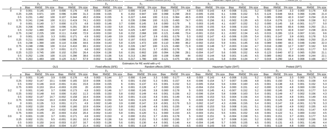
Table 1 gives the bias, RMSE, and size of tests for𝐻𝑎

0 :𝛽3 = 1,and𝐻0𝑏 :𝛾2 =

1 at the 5% signiﬁcance level. This is done for (𝑁 = 100, 𝑇 = 3) in an SHT world where 𝜓 = 1 in the upper panel of Table 1 and an SRE world where

𝜓 = 0 in the lower panel of Table 1. Consider the SHT world conﬁguration where 𝜌 = 0 (no spatial correlation) and increasing heterogeneity through

𝜙 ∈ {0; 0.25; 0.50; 0.75} in Table 1. Obviously, with correlation between some regressors and the individual eﬀects, OLS and SRE are consistent only if 𝜙 = 0 (no random individual eﬀects correlated with the regressors). If

𝜙 > 0, the endogeneity of X𝐶𝑡 and Z𝐶 will lead to parameter bias. Note

that the bias and RMSE for OLS and SRE increase with 𝜙 and the size of the tests for 𝐻𝑎

0 : 𝛽3 = 1 and 𝐻0𝑏 :𝛾2 = 1 is unacceptable, rejecting the null

when true up to 100% of the time, especially when 𝜙 > 0.5. This conﬁrms the results in Baltagi, Bresson, and Pirotte (2003). SFE performs well for𝛽3

but does not yield estimates for 𝛾2. The SHT estimator yields a low RMSE

for both 𝛽3 and 𝛾2.

If 𝜌 ∕= 0 (spatial correlation), OLS is consistent but ineﬃcient at 𝜙 = 0. Of course, OLS is inconsistent if 𝜙 > 0 with endogenous regressors. SHT delivers consistent and asymptotically eﬃcient estimates of both 𝛽3 and 𝛾2

at 𝜙 > 0 and 𝜌 ∕= 0, while SFE yields consistent estimates for 𝛽3 only. In

Table 1, for𝜌= 0.6 and𝜙= 0.5, the RMSE of𝛽3 for OLS is 1.156 compared

(15)

RMSE of 𝛾2 for OLS is 0.286 compared to 0.368 for SRE and 0.145 for SHT.

Tests of hypotheses are misleading with OLS and SRE unless 𝜙= 0 but are properly sized for SFE and SHT at 𝜙 >0 and 𝜌∕= 0.

In an SRE world as in the lower panel of Table 1, there is no correlation between the regressors and the individual eﬀects (𝜓 = 0). In this case, the SRE estimator gives a lower RMSE for𝛽3than OLS, SFE, or SHT, especially

with 𝜙 >0 and as 𝜙 increases. This is also true for𝛾2 when comparing SRE

to OLS or SHT. However, SHT is not far behind SRE in RMSE performance even if the true world is SRE.

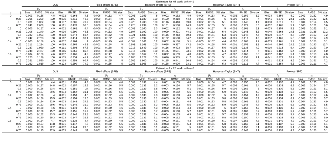
In Table 2, we hold𝑁 constant at 100 and increase 𝑇 from 3 to 5, while in Table 3, we hold 𝑇 constant at 3 but increase 𝑁 from 100 to 300. The purpose of these tables is to see how different sample sizes and time periods affect the performance of the estimators. By and large, we observe the same results as in Table 1, but with different bias and RMSE magnitudes. In general, the SHT and SFE estimators perform best in an SHT world, and the SRE and SHT estimators perform best in an SRE world in terms of RMSE.

In Tables 1-3, we considered the two cases of 𝜓 = 0 or 1. In Table 4, we repeat the results from those tables for two alternative values of spatial autocorrelation, 𝜌∈ {0.2,0.4}, and for a sample size of 𝑁 = 100 and 𝑇 = 3 but at values of 𝜓 ∈ {0,0.1,0.25,0.5,1}. The purpose of this table is to illustrate how the performance of the estimators changes with the degree of correlation between the regressors and the individual eﬀects. In fact, the average correlation between 𝜇 and 𝑋𝑐 and 𝑍𝑐 amounts to 0.928 and 0.519,

respectively, at a true value of 𝜓 = 1 and 𝜙 = 0.5 and to 0.652 and 0.365, respectively, at a true value of 𝜓 = 0.5 and 𝜙= 0.5. The results suggest that the SHT estimator outperforms the SRE and OLS estimators as 𝜓 increases.

(16)

3.3 The Spatial Pretest Estimator

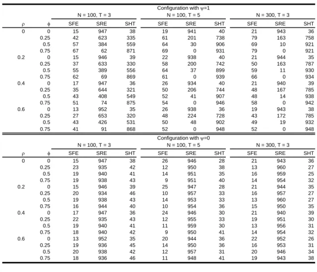
Table 5 shows the choice of the SPT estimator for various values of 𝜌 and 𝜙

corresponding to the results in Tables 1-3 at values of𝜓 = 1 (SHT world) and

𝜓 = 0 (SRE world). The upper left panel in Table 5 provides the results for (𝑁 = 100, 𝑇 = 3) for an SHT world. For example, at𝜌 = 0.4 and 𝜙 = 0.75, the SPT estimator is an SHT estimator in 875 out of 1,000 replications, an SFE estimator in 51 replications, and an SRE estimator in the remaining 74 replications. As 𝜙, N or T increases, the SPT estimator picks the SHT estimator more frequently. The performance of the SPT estimator reported in the upper panel of Table 1 is in between the SHT and the SRE estimators in terms of RMSE for both 𝛽3 and 𝛾2. The size of tests for 𝐻0𝑎 : 𝛽3 = 1,

and 𝐻𝑏

0 :𝛾2 = 1 for SPT are obviously aﬀected by the pretesting and are not

recommended in practice.5

In the lower panel of Table 5, we show the choice of the SPT estimator for various values of 𝜌 and 𝜙 corresponding to the results in Tables 1-3 in an SRE world. For example, at 𝜌 = 0.4, 𝜙 = 0.75, and (𝑁 = 100, 𝑇 = 3), the SPT estimator is an SRE estimator in 940 out of 1,000 replications, an SFE estimator in 18 replications, and an SHT estimator in the remaining 42 replications. As 𝑁 or 𝑇 increases, the SPT estimator picks the SRE estimator more frequently. The performance of the SPT estimator reported

5_{It is well known that the pretest estimator (based on the Hausman test in the ﬁrst step}

and a simple hypothesis test in the second step) displays poor size and power properties, see Guggenberger (2010). This is confirmed by Baltagi, Bresson, and Pirotte (2003) using standard panel data Monte Carlo experiments and by our results here for their spatial counterparts. In fact, Guggenberger’s (2010) recommendation of using a (one-step) t-test procedure based on the fixed effects estimator instead of a two-step procedure is a good idea even under the presence of spatial correlation. In this case, the researcher would use the t-test based on the SFE estimator instead of the two-stage procedure.

(17)

in the lower panel of Table 1 is in between the SRE and the SFE estimator in terms of RMSE for 𝛽3. Again, the size of tests for 𝐻0𝑎 : 𝛽3 = 1, and 𝐻₀𝑏 :𝛾2 = 1 for SPT are obviously aﬀected by the pretesting.

4 Conclusions

This paper provides Monte Carlo evidence on the small sample performance of Cliff and Ord (1973) type spatial panel data estimators. We focus on Haus-man and Taylor (1981) type panel data models with spatial disturbances. We find that the spatial Hausman and Taylor type estimator performs well in terms of root mean squared error in comparison to the spatial fixed effects, the spatial random effects, and the OLS estimators. An added advantage of the spatial Hausman-Taylor estimator is that it delivers estimates of endoge-nous time-invariant variables, unlike the spatial fixed effects model. Unlike the spatial random effects or the pooled OLS model, it allows regressors in the model to be correlated with the individual-specific effects.

We also investigate the performance of a spatial pretest estimator based on two Hausman tests. We find that the spatial pretest estimators perform particularly well if the heterogeneity due to the individual effects is relatively important and the associated problem of endogeneity of the regressors with the individual effects becomes more pertinent. The spatial pretest estimator guards against a possible misspecified choice of estimator and its RMSE performance is satisfactory, but tests of hypotheses using the SHT estimator are not recommended. Instead one should use the one-step SFE in practice, but unfortunately this applies to the time-varying regressor coefficients only.6

6_{Modern approaches to causal inﬂuence queries should be deﬁned dynamically and}

should recognize the role of time in causality. This is an important problem for future research but is beyond the scope of this paper.

(18)

Appendix

All of the Monte Carlo runs are based on the following unnormalized weights matrix based on a three-before-and-three-behind design of neighborhood

W0 = ⎛ ⎜ ⎜ ⎜ ⎜ ⎜ ⎜ ⎜ ⎜ ⎜ ⎜ ⎜ ⎜ ⎜ ⎜ ⎜ ⎜ ⎜ ⎜ ⎜ ⎜ ⎜ ⎜ ⎝ 0 1 1 1 0 ⋅ ⋅ ⋅ 0 1 1 1 1 0 1 1 1 0 ⋅ ⋅ ⋅ 0 1 1 1 1 0 1 1 1 0 ⋅ ⋅ ⋅ 0 1 1 1 1 0 1 1 1 0 ⋅ ⋅ ⋅ 0 0 1 1 1 0 1 1 1 0 0 .. . ... ... ... ... 0 ... ... ... ... 0 ⋅ ⋅ ⋅ 0 1 1 1 0 1 1 1 1 1 ⋅ ⋅ ⋅ 0 1 1 1 0 1 1 1 1 0 ⋅ ⋅ ⋅ 0 1 1 1 0 1 1 1 1 0 ⋅ ⋅ ⋅ 0 1 1 1 0 ⎞ ⎟ ⎟ ⎟ ⎟ ⎟ ⎟ ⎟ ⎟ ⎟ ⎟ ⎟ ⎟ ⎟ ⎟ ⎟ ⎟ ⎟ ⎟ ⎟ ⎟ ⎟ ⎟ ⎠ .

Each row of this matrix exhibits a row-sum of 6. Hence, the row-normalized as well as the maximum row-sum normalized counterpart of that matrix is

W= ⎛ ⎜ ⎜ ⎜ ⎜ ⎜ ⎜ ⎜ ⎜ ⎜ ⎜ ⎜ ⎜ ⎜ ⎜ ⎜ ⎜ ⎜ ⎜ ⎜ ⎜ ⎜ ⎜ ⎝ 0 1/6 1/6 1/6 0 ⋅ ⋅ ⋅ 0 1/6 1/6 1/6 1/6 0 1/6 1/6 1/6 0 ⋅ ⋅ ⋅ 0 1/6 1/6 1/6 1/6 0 1/6 1/6 1/6 0 ⋅ ⋅ ⋅ 0 1/6 1/6 1/6 1/6 0 1/6 1/6 1/6 0 ⋅ ⋅ ⋅ 0 0 1/6 1/6 1/6 0 1/6 1/6 1/6 0 0 .. . ... ... ... ... 0 ... ... ... ... 0 ⋅ ⋅ ⋅ 0 1/6 1/6 1/6 0 1/6 1/6 1/6 1/6 1/6 ⋅ ⋅ ⋅ 0 1/6 1/6 1/6 0 1/6 1/6 1/6 1/6 0 ⋅ ⋅ ⋅ 0 1/6 1/6 1/6 0 1/6 1/6 1/6 1/6 0 ⋅ ⋅ ⋅ 0 1/6 1/6 1/6 0 ⎞ ⎟ ⎟ ⎟ ⎟ ⎟ ⎟ ⎟ ⎟ ⎟ ⎟ ⎟ ⎟ ⎟ ⎟ ⎟ ⎟ ⎟ ⎟ ⎟ ⎟ ⎟ ⎟ ⎠ .

(19)

References

Baltagi, B. H. (2008). Econometric Analysis of Panel Data, Wiley: New York.

Baltagi, B. H., Bresson, G. and Pirotte, A. (2003). Fixed eﬀects, random eﬀects or Hausman-Taylor? A pretest estimator. Economics Letters

79, 361-369.

Baltagi, B. H., Egger, P. H. and Kesina, M. (2011). Firm-level Productivity Spillovers in China’s Chemical Industry: A Spatial Hausman-Taylor Approach, working paper.

Cliﬀ, A. and J. Ord. (1973), Spatial Autocorrelation, Pion, London. Contoyannis, P. and Rice, N. (2001). The impact of health on wages:

Ev-idence form the British household panel survey. Empirical Economics

26, 599-622.

Cornwell, C. and Rupert, P. (1988). Eﬃcient estimation with panel data: an empirical comparison of instrumental variables estimators. Journal of Applied Econometrics 3, 149-155.

Debarsy, N. (2012). The Mundlak approach in the spatial Durbin panel data model, Spatial Economic Analysis 7, 109-131.

Egger, P. (2004). On the problem of endogenous unobserved eﬀects in the estimation of gravity models. Journal of Economic Integration 19, 182-191.

Egger, P. and Pfaﬀermayr, M. (2004). Distance, trade and FDI: a Hausman-Taylor SUR approach. Journal of Applied Econometrics 19, 227-246.

(20)

Ertur, C. and Koch, W. (2007). Growth, technological interdependence and spatial externalities: Theory and evidence, Journal of Applied Econo-metrics 22, 1033–1062.

Ertur, C. and Koch, W. (2011). A contribution to the Schumpeterian growth theory and empirics. Journal of Economic Growth 16, 215– 255.

Guggenberger, P. (2010). The impact of a Hausman pretest on the size of a hypothesis test: The panel data case. Journal of Econometrics 156, 337-343.

Hausman, J.A. (1978). Speciﬁcation tests in econometrics. Econometrica

46, 1251-1271.

Hausman, J.A. and Taylor, W.E. (1981). Panel data and unobservable individual eﬀects. Econometrica 49, 1377-1398.

Kapoor, M., Kelejian, H.H. and Prucha, I. (2007). Panel data models with spatially correlated error components. Journal of Econometrics 140, 97-130.

Light, A. and Ureta, M. (1995). Early-career work experience and gender wage diﬀerentials. Journal of Labor Economics 13, 121-154.

Mutl, J. and Pfaﬀermayr, M. (2011). The Hausman test in a Cliﬀ and Ord panel model. Econometrics Journal 14, 48-76.

Pfaﬀermayr, M. (2009). Conditional beta and sigma convergence in space: A maximum likelihood approach, Regional Science and Urban Eco-nomics 39, 63–78.

(21)

Serlenga, L. and Shin, Y. (2007). Gravity models of intra-EU trade: appli-cation of the CCEP-HT estimation in heterogeneous panels with unob-served common time-speciﬁc factors. Journal of Applied Econometrics

(22)

Table 1 - Bias, RMSE and 5% test size, N=100 and T=3

  Bias RMSE 5% size Bias RMSE 5% size Bias RMSE 5% size Bias RMSE 5% size Bias RMSE 5% size Bias RMSE 5% size Bias RMSE 5% size Bias RMSE 5% size Bias RMSE 5% size

0 0 0.001 0.145 3.9 0.000 0.176 4.8 0.003 0.144 3.7 0.000 0.144 3.3 0.000 0.177 4.8 0.003 0.143 4.4 -0.008 0.151 5.2 0.000 0.144 3.3 0.000 0.176 4.8 0.25 0.205 0.971 100 0.096 0.289 31.3 -0.006 0.155 6 0.202 0.947 100 0.098 0.298 29.9 -0.005 0.155 6.1 0.006 0.152 5.5 0.124 0.648 64.6 0.066 0.246 21.4 0.5 0.231 1.492 100 0.107 0.344 49.2 -0.004 0.155 6 0.227 1.444 100 0.111 0.364 46.5 -0.003 0.156 6.3 0.002 0.144 5 0.085 0.650 42.3 0.047 0.234 21.9 0.75 0.241 2.246 100 0.111 0.419 74.1 -0.003 0.155 6 0.235 2.096 100 0.121 0.493 74.7 -0.001 0.156 6.1 -0.002 0.135 4.5 0.014 0.276 11.9 0.006 0.158 9.2 0.2 0 0.001 0.140 3.7 0.000 0.173 4.8 0.003 0.146 3.7 0.000 0.145 3.8 0.000 0.178 5 0.003 0.145 4.1 -0.007 0.152 5.2 0.000 0.145 3.8 -0.001 0.177 5.0 0.25 0.206 0.965 100 0.096 0.291 30.9 -0.005 0.150 5.8 0.201 0.930 100 0.098 0.300 29.3 -0.005 0.155 6.4 0.006 0.153 5.5 0.125 0.646 65.6 0.066 0.250 21.1 0.5 0.232 1.480 100 0.107 0.347 48.4 -0.004 0.150 5.8 0.225 1.487 100 0.111 0.372 47.5 -0.003 0.155 6.5 0.002 0.144 5.2 0.086 0.673 42.8 0.047 0.238 22.6 0.75 0.242 2.225 100 0.111 0.430 72.9 -0.003 0.150 5.8 0.232 2.068 100 0.121 0.496 73.4 -0.001 0.153 6.1 -0.002 0.134 4.5 0.015 0.285 12.6 0.007 0.161 9.6 0.4 0 0.001 0.135 3.3 0.001 0.171 4.9 0.002 0.149 3.9 0.000 0.147 3.9 -0.001 0.179 5.3 0.002 0.147 4.3 -0.006 0.155 5.4 0.001 0.147 3.9 -0.001 0.178 5.3 0.25 0.211 0.890 100 0.098 0.286 30.1 -0.004 0.143 5.8 0.197 0.915 100 0.096 0.298 29.3 -0.004 0.153 5.9 0.006 0.152 5.7 0.125 0.644 66.5 0.066 0.250 21.4 0.5 0.238 1.390 100 0.110 0.336 44.6 -0.004 0.143 5.8 0.220 1.472 100 0.110 0.369 46.2 -0.002 0.153 5.9 0.001 0.145 4.6 0.089 0.690 44.3 0.048 0.240 22.3 0.75 0.248 2.096 100 0.114 0.410 69.1 -0.002 0.143 5.8 0.226 1.947 100 0.121 0.490 71.9 0.000 0.148 5.7 -0.003 0.134 4.7 0.016 0.280 12.7 0.007 0.162 9.9 0.6 0 0.001 0.130 3.7 0.001 0.171 4.8 0.002 0.153 4 0.000 0.151 3.7 -0.001 0.178 5 0.002 0.151 5 -0.004 0.158 5.1 0.001 0.151 3.7 -0.001 0.177 5.0 0.25 0.223 0.745 100 0.102 0.250 26.4 -0.004 0.136 5.6 0.191 0.902 100 0.094 0.298 29.1 -0.004 0.147 5.6 0.005 0.152 4.9 0.123 0.640 67.2 0.065 0.250 21.1 0.5 0.252 1.156 100 0.115 0.286 38.6 -0.003 0.136 5.6 0.213 1.360 100 0.108 0.368 44 -0.002 0.144 5.8 0.001 0.145 4.5 0.089 0.662 45.9 0.049 0.244 22.1 0.75 0.263 1.483 100 0.120 0.317 57.9 -0.002 0.136 5.6 0.217 1.780 100 0.121 0.475 68.4 0.000 0.141 5.8 -0.004 0.134 4.7 0.019 0.290 14.4 0.008 0.166 10.7

0 0 0.001 0.145 3.9 0.000 0.176 4.8 0.003 0.144 3.7 0.000 0.144 3.3 0.000 0.177 4.8 0.003 0.143 4.4 -0.008 0.151 5.2 0.000 0.144 3.3 0.000 0.176 4.8 0.25 0.002 0.147 10.1 0.000 0.165 10.9 -0.006 0.155 6 0.001 0.150 5.3 0.001 0.157 4.4 -0.006 0.154 5.7 0.007 0.166 4.8 0.001 0.150 5.3 0.001 0.158 4.4 0.5 0.002 0.146 14.8 -0.001 0.161 15.8 -0.004 0.155 6 0.001 0.137 4.5 0.001 0.152 5.3 -0.005 0.154 5.6 0.004 0.160 4.5 0.001 0.138 4.6 0.001 0.152 5.3 0.75 0.003 0.153 19.4 -0.003 0.155 20 -0.003 0.155 6 0.001 0.128 4.7 0.000 0.150 5.5 -0.004 0.153 5.4 0.000 0.151 4.2 0.000 0.129 4.8 0.000 0.150 5.4 0.2 0 0.001 0.140 3.7 0.000 0.173 4.8 0.003 0.146 3.7 0.000 0.145 3.8 0.000 0.178 5 0.003 0.145 4.1 -0.007 0.152 5.2 0.000 0.145 3.8 -0.001 0.177 5.0 0.25 0.002 0.148 9.6 0.000 0.162 11.3 -0.005 0.150 5.8 0.002 0.149 4.6 0.001 0.156 4.2 -0.006 0.154 5.8 0.008 0.163 5.4 0.001 0.149 4.7 0.002 0.156 4.3 0.5 0.002 0.147 14.7 -0.002 0.158 16.4 -0.004 0.150 5.8 0.001 0.133 4.8 0.001 0.149 4.6 -0.005 0.153 5.5 0.004 0.156 4.4 0.001 0.134 4.8 0.001 0.149 4.6 0.75 0.003 0.154 19.3 -0.003 0.154 20.4 -0.003 0.150 5.8 0.001 0.123 4.8 0.000 0.151 5 -0.003 0.152 5.3 0.001 0.151 4.4 0.001 0.125 4.8 0.000 0.151 5.0 0.4 0 0.001 0.135 3.3 0.001 0.171 4.9 0.002 0.149 3.9 0.000 0.147 3.9 -0.001 0.179 5.3 0.002 0.147 4.3 -0.006 0.155 5.4 0.001 0.147 3.9 -0.001 0.178 5.3 0.25 0.002 0.150 9.4 0.000 0.160 10.9 -0.004 0.143 5.8 0.002 0.149 4.8 0.001 0.155 4 -0.005 0.153 5.6 0.008 0.161 5.1 0.001 0.149 4.9 0.002 0.155 4.0 0.5 0.003 0.149 14.2 -0.002 0.156 16.6 -0.004 0.143 5.8 0.001 0.131 4.5 0.001 0.147 4.9 -0.004 0.153 5.3 0.005 0.155 4.4 0.001 0.132 4.6 0.001 0.147 4.9 0.75 0.003 0.155 20 -0.003 0.153 20.4 -0.002 0.143 5.8 0.001 0.120 5.1 0.000 0.153 4.5 -0.003 0.151 5.5 0.001 0.152 4.6 0.001 0.122 5.1 0.000 0.153 4.5 0.6 0 0.001 0.130 3.7 0.001 0.171 4.8 0.002 0.153 4 0.000 0.151 3.7 -0.001 0.178 5 0.002 0.151 5 -0.004 0.158 5.1 0.001 0.151 3.7 -0.001 0.177 5.0 0.25 0.002 0.151 9.5 -0.001 0.161 10.3 -0.004 0.136 5.6 0.002 0.151 5.3 0.002 0.155 3.7 -0.005 0.147 5.7 0.008 0.161 5.2 0.001 0.150 5.3 0.002 0.155 3.8 0.5 0.003 0.150 14.6 -0.003 0.157 16.7 -0.003 0.136 5.6 0.001 0.130 4.4 0.001 0.146 4.4 -0.004 0.146 5.7 0.005 0.155 4.5 0.001 0.131 4.5 0.001 0.146 4.4 0.75 0.003 0.156 20.6 -0.004 0.157 21.4 -0.002 0.136 5.6 0.001 0.118 4.7 0.000 0.151 4.5 -0.003 0.143 5.9 0.001 0.152 4 0.001 0.119 4.8 0.000 0.151 4.5 3 2 Pretest (SPT) 3 2 Pretest (SPT) 3 2 3 2 3 2 3

Estimators for RE world with =0

OLS Fixed effects (SFE) Random effects (SRE) Hausman-Taylor (SHT)

Estimators for HT world with =1

(23)

0 0 -0.003 0.158 4.8 0.002 0.163 4.8 -0.006 0.152 4.7 -0.003 0.159 5 0.002 0.162 4.9 -0.006 0.153 5.1 -0.002 0.159 5.2 -0.003 0.159 5.0 0.002 0.162 4.9 0.25 0.205 1.209 100 0.095 0.311 46.3 0.000 0.164 4.9 0.199 1.180 100 0.100 0.318 44.2 0.001 0.166 5 0.000 0.145 4 0.041 0.370 24.1 0.022 0.182 12.6 0.5 0.231 1.822 100 0.107 0.381 70.7 0.000 0.164 4.9 0.223 1.703 100 0.116 0.413 69.8 0.002 0.165 5.1 0.000 0.146 4.4 0.008 0.211 7.9 0.004 0.154 6.5 0.75 0.241 2.609 100 0.111 0.478 90.6 0.000 0.164 4.9 0.228 2.239 100 0.131 0.568 94.3 0.002 0.165 5.1 0.000 0.121 5.6 0.002 0.165 5.1 0.000 0.121 5.6 0.2 0 -0.003 0.157 4.9 0.002 0.162 4.4 -0.006 0.153 4.7 -0.003 0.160 5.3 0.002 0.162 5.1 -0.006 0.157 5 -0.002 0.161 5.1 -0.003 0.159 5.3 0.002 0.162 5.1 0.25 0.206 1.240 100 0.096 0.290 46.3 -0.001 0.162 4.9 0.197 1.192 100 0.099 0.321 44.1 0.001 0.162 5.4 0.000 0.148 3.6 0.040 0.368 24.3 0.021 0.185 12.2 0.5 0.232 1.993 100 0.108 0.344 69.4 -0.001 0.162 4.9 0.221 1.683 100 0.116 0.413 69.3 0.001 0.161 5.3 -0.001 0.142 4.6 0.009 0.217 8.8 0.004 0.152 7.2 0.75 0.242 2.733 100 0.112 0.414 90.4 0.000 0.162 4.9 0.225 2.194 100 0.132 0.568 94.2 0.002 0.161 5.3 -0.001 0.117 4.9 0.002 0.161 5.3 -0.001 0.117 4.9 0.4 0 -0.003 0.158 4.5 0.002 0.164 4 -0.005 0.149 4.6 -0.002 0.161 5.2 0.002 0.160 5.1 -0.005 0.157 4.4 -0.002 0.163 4.7 -0.003 0.161 5.2 0.002 0.160 5.1 0.25 0.211 1.224 100 0.099 0.265 45.2 -0.001 0.158 5 0.193 1.168 100 0.098 0.327 43.2 0.000 0.158 5.5 -0.001 0.152 3.8 0.040 0.366 24.9 0.021 0.190 12.3 0.5 0.237 1.950 100 0.111 0.303 67.8 -0.001 0.158 5 0.215 1.649 100 0.116 0.423 68.7 0.001 0.157 5.6 -0.002 0.138 4.2 0.010 0.218 9.4 0.004 0.150 7.0 0.75 0.248 2.487 100 0.115 0.351 85.5 -0.001 0.158 5 0.217 2.109 100 0.135 0.591 93.1 0.002 0.158 5.4 -0.002 0.114 5 0.001 0.158 5.4 -0.002 0.114 5.0 0.6 0 -0.004 0.160 4.6 0.002 0.166 4.2 -0.005 0.147 4.5 -0.002 0.162 5.1 0.002 0.159 4.8 -0.005 0.159 4.7 -0.002 0.162 5.3 -0.002 0.162 5.1 0.002 0.159 4.8 0.25 0.223 1.136 100 0.105 0.234 41.1 -0.001 0.155 5 0.186 1.127 100 0.096 0.335 41.7 0.000 0.155 5.1 -0.001 0.153 4.1 0.041 0.373 26.4 0.022 0.196 12.9 0.5 0.251 1.520 100 0.118 0.259 60.7 -0.001 0.155 5 0.206 1.600 100 0.115 0.441 66.8 0.001 0.154 4.9 -0.002 0.135 4 0.011 0.223 9.5 0.004 0.151 7.2 0.75 0.262 1.819 100 0.123 0.290 74.9 -0.001 0.155 5 0.205 1.965 100 0.138 0.600 93.1 0.001 0.154 5.3 -0.003 0.111 4.7 0.001 0.154 5.3 -0.003 0.111 4.7

0 0 0.002 0.131 4.4 0.001 0.159 4.9 0.000 0.154 4.6 0.002 0.131 4.4 0.001 0.155 4.8 0.000 0.154 4.7 0.005 0.150 4.6 0.002 0.132 4.4 0.002 0.155 4.8 0.25 0.000 0.157 14.8 -0.002 0.157 15.8 0.001 0.156 5.5 0.000 0.132 6.2 -0.003 0.154 5.7 0.001 0.155 5.7 -0.006 0.161 5.4 0.000 0.133 6.2 -0.003 0.154 5.7 0.5 0.000 0.156 23.4 -0.003 0.151 24 0.001 0.156 5.5 0.000 0.129 5.8 -0.004 0.150 5.1 0.001 0.156 5.9 -0.006 0.162 5 0.000 0.130 5.8 -0.004 0.151 5.1 0.75 0.000 0.157 29.6 -0.004 0.152 31.1 0.000 0.156 5.5 0.000 0.132 5.5 -0.005 0.152 5.5 0.000 0.156 5.9 -0.005 0.146 4.9 0.000 0.134 5.5 -0.005 0.152 5.5 0.2 0 0.002 0.130 4 0.001 0.153 4.6 0.000 0.152 4.6 0.002 0.133 4.3 0.002 0.163 4.6 0.000 0.152 5 0.006 0.151 4.9 0.002 0.134 4.3 0.002 0.162 4.6 0.25 0.000 0.156 15.5 -0.002 0.154 15.6 0.001 0.153 5.5 0.000 0.133 6.1 -0.003 0.158 5.7 0.001 0.153 5.8 -0.006 0.161 5.2 0.000 0.134 6.1 -0.003 0.158 5.7 0.5 0.000 0.154 22.9 -0.003 0.148 24.6 0.001 0.153 5.5 0.000 0.130 5.7 -0.004 0.151 4.9 0.001 0.153 5.8 -0.006 0.161 5.2 0.000 0.131 5.7 -0.004 0.152 4.9 0.75 0.000 0.153 29.6 -0.004 0.149 31.9 0.000 0.153 5.5 0.000 0.133 5.3 -0.005 0.152 5.5 0.000 0.153 5.9 -0.005 0.148 4.7 0.000 0.134 5.3 -0.005 0.152 5.5 0.4 0 0.002 0.130 4.6 0.001 0.149 4.8 0.000 0.150 4.6 0.002 0.135 4.3 0.002 0.164 4.4 0.000 0.150 5 0.007 0.153 4.7 0.002 0.136 4.3 0.002 0.164 4.4 0.25 0.000 0.156 15.7 -0.002 0.151 15.7 0.001 0.152 5.5 0.000 0.134 5.7 -0.003 0.160 5.7 0.001 0.151 5.9 -0.005 0.162 5.2 0.000 0.135 5.7 -0.003 0.161 5.7 0.5 0.000 0.152 23.3 -0.003 0.146 23.8 0.001 0.152 5.5 0.000 0.132 5.4 -0.004 0.153 4.9 0.001 0.151 5.7 -0.005 0.158 5.2 0.000 0.133 5.4 -0.004 0.153 4.9 0.75 0.001 0.150 29.3 -0.003 0.147 32.8 0.001 0.152 5.5 0.000 0.132 5.1 -0.005 0.152 5 0.001 0.152 5.8 -0.005 0.150 4.4 0.000 0.133 5.1 -0.005 0.152 5.0 0.6 0 0.002 0.134 4.7 0.000 0.138 4.4 0.000 0.150 4.8 0.002 0.140 4.1 0.002 0.161 4.3 0.000 0.150 5.1 0.007 0.153 4.8 0.001 0.140 4.2 0.002 0.161 4.3 0.25 0.000 0.157 14.8 -0.001 0.147 16 0.001 0.152 5.5 0.000 0.136 5.5 -0.003 0.161 5.4 0.001 0.151 5.8 -0.005 0.162 5.1 0.000 0.137 5.5 -0.003 0.161 5.4 0.5 0.000 0.150 22.2 -0.002 0.144 23.6 0.001 0.152 5.5 0.000 0.132 5.1 -0.004 0.151 5 0.001 0.151 5.9 -0.005 0.153 5.1 0.000 0.133 5.1 -0.004 0.151 5.0 0.75 0.001 0.145 27.9 -0.003 0.143 32 0.001 0.152 5.5 0.000 0.132 4.9 -0.005 0.150 5.1 0.001 0.151 5.8 -0.005 0.148 4.1 0.000 0.133 4.9 -0.005 0.150 5.1 3 2 3 2 3 2 3 2 3

OLS Fixed effects (SFE) Random effects (SRE) Hausman-Taylor (SHT) Pretest (SPT)

(24)

0 0 -0.001 0.165 4.8 0.001 0.176 6.8 -0.002 0.167 6.3 -0.001 0.166 4.9 0.001 0.176 5.9 -0.002 0.168 6.5 0.001 0.142 5 -0.001 0.166 5.0 0.001 0.175 5.9 0.25 0.207 1.615 100 0.095 0.454 71.8 -0.003 0.157 4.8 0.204 1.596 100 0.097 0.477 70.9 -0.002 0.155 5.1 0.003 0.162 5 0.031 0.390 20.5 0.020 0.217 16.7 0.5 0.232 2.492 100 0.106 0.591 91.5 -0.002 0.157 4.8 0.228 2.496 100 0.110 0.619 91.6 -0.002 0.156 5.1 0.003 0.167 4.5 0.001 0.179 6.0 0.004 0.172 5.4 0.75 0.242 3.735 100 0.110 0.755 99.7 -0.002 0.157 4.8 0.236 3.558 100 0.120 0.796 99.7 -0.001 0.157 4.9 0.003 0.171 4.5 -0.001 0.157 4.9 0.003 0.171 4.5 0.2 0 -0.001 0.167 4.9 0.001 0.173 6.4 -0.002 0.166 5.7 -0.001 0.167 5.2 0.000 0.177 5.9 -0.002 0.167 5.9 0.000 0.142 5.2 -0.001 0.167 5.2 0.000 0.175 5.9 0.25 0.208 1.622 100 0.096 0.461 71.6 -0.003 0.152 5.4 0.203 1.585 100 0.096 0.459 70.6 -0.003 0.151 5.7 0.003 0.160 4.9 0.031 0.385 21.1 0.019 0.212 16.2 0.5 0.233 2.507 100 0.107 0.583 90.9 -0.002 0.152 5.4 0.227 2.400 100 0.110 0.618 90.3 -0.002 0.152 5.6 0.003 0.160 4.9 0.001 0.176 6.6 0.004 0.165 5.9 0.75 0.243 3.729 100 0.111 0.746 99.5 -0.002 0.152 5.4 0.233 3.486 100 0.120 0.794 99.7 -0.001 0.152 5.4 0.003 0.162 5.1 -0.001 0.152 5.4 0.003 0.162 5.1 0.4 0 -0.001 0.172 5.5 0.001 0.172 6.2 -0.002 0.167 5.1 -0.001 0.169 5 0.000 0.176 5.4 -0.002 0.167 5.6 -0.001 0.142 5.6 -0.001 0.169 5.0 0.000 0.175 5.4 0.25 0.214 1.559 100 0.098 0.450 69.5 -0.003 0.149 5.4 0.199 1.534 100 0.094 0.441 69.3 -0.003 0.149 5.8 0.002 0.156 4.8 0.031 0.380 21.5 0.018 0.206 16.1 0.5 0.240 2.453 100 0.110 0.561 89.5 -0.003 0.149 5.4 0.222 2.317 100 0.108 0.591 89.1 -0.002 0.149 5.7 0.002 0.154 5 0.001 0.179 7.0 0.004 0.160 6.2 0.75 0.250 3.481 100 0.114 0.649 98.2 -0.002 0.149 5.4 0.227 3.365 100 0.119 0.787 99.6 -0.001 0.149 5.8 0.002 0.155 5.2 -0.001 0.149 5.8 0.002 0.155 5.2 0.6 0 -0.001 0.163 4.9 0.002 0.172 6.4 -0.002 0.167 5.3 -0.001 0.167 5.2 0.000 0.174 4.7 -0.002 0.166 5.7 -0.002 0.142 5.8 -0.001 0.167 5.2 0.000 0.173 4.7 0.25 0.227 1.473 100 0.105 0.412 64 -0.003 0.147 5.5 0.192 1.500 100 0.091 0.422 66.3 -0.003 0.147 5.8 0.002 0.152 4.7 0.030 0.380 22.0 0.018 0.200 15.8 0.5 0.255 2.243 100 0.117 0.475 83.1 -0.003 0.147 5.5 0.214 2.284 100 0.105 0.564 87.3 -0.002 0.147 5.8 0.002 0.148 5.5 0.002 0.188 7.6 0.004 0.157 7.1 0.75 0.265 2.567 100 0.122 0.514 93.8 -0.002 0.147 5.5 0.217 3.357 100 0.118 0.784 99.5 -0.001 0.147 5.7 0.002 0.150 5.2 -0.001 0.147 5.7 0.002 0.150 5.2

0 0 -0.001 0.165 4.8 0.001 0.176 6.8 -0.002 0.167 6.3 -0.001 0.166 4.9 0.001 0.176 5.9 -0.002 0.168 6.5 0.001 0.142 5 -0.001 0.166 5.0 0.001 0.175 5.9 0.25 -0.001 0.129 9.8 0.001 0.158 10.9 -0.003 0.157 4.8 -0.001 0.134 5 0.001 0.154 5.8 -0.003 0.157 5.1 0.003 0.162 5.2 -0.001 0.135 5.0 0.001 0.155 5.8 0.5 -0.001 0.131 15.3 0.000 0.159 15.3 -0.002 0.157 4.8 -0.001 0.139 5.5 0.001 0.160 5.5 -0.002 0.157 5.1 0.003 0.159 4.5 -0.001 0.139 5.5 0.001 0.160 5.5 0.75 -0.001 0.144 19 0.000 0.160 19.3 -0.002 0.157 4.8 -0.001 0.159 5.4 0.001 0.155 5.7 -0.002 0.157 5 0.003 0.155 4.7 -0.001 0.159 5.4 0.001 0.155 5.7 0.2 0 -0.001 0.167 4.9 0.001 0.173 6.4 -0.002 0.166 5.7 -0.001 0.167 5.2 0.000 0.177 5.9 -0.002 0.167 5.9 0.000 0.142 5.2 -0.001 0.167 5.2 0.000 0.175 5.9 0.25 -0.001 0.128 9.3 0.001 0.154 11 -0.003 0.152 5.4 -0.001 0.133 5.5 0.001 0.161 5.5 -0.003 0.153 5.7 0.003 0.160 4.7 -0.001 0.134 5.5 0.001 0.161 5.5 0.5 -0.001 0.129 15.6 0.001 0.154 15.2 -0.002 0.152 5.4 -0.001 0.139 5.6 0.001 0.163 5.2 -0.003 0.153 5.5 0.003 0.156 5 -0.001 0.140 5.6 0.001 0.163 5.2 0.75 -0.001 0.141 18.8 0.000 0.159 18.9 -0.002 0.152 5.4 -0.001 0.160 5.4 0.001 0.157 5.6 -0.002 0.153 5.6 0.003 0.153 4.7 -0.001 0.159 5.4 0.001 0.156 5.6 0.4 0 -0.001 0.172 5.5 0.001 0.172 6.2 -0.002 0.167 5.1 -0.001 0.169 5 0.000 0.176 5.4 -0.002 0.167 5.6 -0.001 0.142 5.6 -0.001 0.169 5.0 0.000 0.175 5.4 0.25 -0.001 0.129 9.2 0.001 0.150 11.2 -0.003 0.149 5.4 -0.001 0.133 5.2 0.001 0.168 5.4 -0.003 0.149 5.7 0.003 0.157 4.8 -0.001 0.134 5.2 0.001 0.168 5.4 0.5 -0.001 0.128 15.9 0.001 0.149 14.9 -0.003 0.149 5.4 -0.001 0.141 5.3 0.001 0.165 5.5 -0.003 0.150 5.7 0.003 0.154 5 -0.001 0.141 5.3 0.001 0.164 5.5 0.75 -0.001 0.138 20.4 0.001 0.155 19 -0.002 0.149 5.4 -0.002 0.161 5 0.001 0.159 5 -0.002 0.149 5.4 0.003 0.152 4.6 -0.002 0.160 5.0 0.001 0.159 5.0 0.6 0 0.000 0.179 4 0.000 0.138 4 -0.001 0.150 4.1 0.000 0.152 5 0.001 0.150 5.5 -0.001 0.151 4.4 0.010 0.145 4.3 0.000 0.152 5.0 0.001 0.150 5.5 0.25 0.000 0.163 10.8 0.001 0.137 8.7 -0.002 0.145 5.7 0.000 0.157 6.2 0.001 0.125 3.5 -0.002 0.147 5.6 -0.009 0.150 4.8 0.000 0.156 6.2 0.000 0.125 3.5 0.5 0.000 0.155 15.8 0.001 0.156 13.9 -0.001 0.145 5.7 0.000 0.151 6.2 0.000 0.134 3.2 -0.001 0.148 5.6 -0.008 0.152 4.7 0.000 0.151 6.2 0.000 0.135 3.3 0.75 0.000 0.157 22 0.000 0.156 19.6 -0.001 0.145 5.7 0.000 0.152 5.6 0.000 0.152 3.8 -0.001 0.148 5.6 -0.007 0.154 4.2 0.000 0.151 5.6 0.000 0.152 3.8 3 2 3 2 3 2 3 2 3

(25)

Table 4 - Bias, RMSE and 5% test size, N=100 and T=3, at different correlation levels 

   Bias RMSE 5% size Bias RMSE 5% size Bias RMSE 5% size Bias RMSE 5% size Bias RMSE 5% size Bias RMSE 5% size Bias RMSE 5% size Bias RMSE 5% size Bias RMSE 5% size

0.2 0 0 0.001 0.140 3.7 0.000 0.173 4.8 0.003 0.146 3.7 0.000 0.145 3.8 0.000 0.178 5 0.003 0.145 4.1 -0.007 0.152 5.2 0.000 0.145 3.8 -0.001 0.177 5.0 0.25 0.002 0.148 9.6 0.000 0.162 11.3 -0.005 0.150 5.8 0.002 0.149 4.6 0.001 0.156 4.2 -0.006 0.154 5.8 0.008 0.163 5.4 0.001 0.149 4.7 0.002 0.156 4.3 0.5 0.002 0.147 14.7 -0.002 0.158 16.4 -0.004 0.150 5.8 0.001 0.133 4.8 0.001 0.149 4.6 -0.005 0.153 5.5 0.004 0.156 4.4 0.001 0.134 4.8 0.001 0.149 4.6 0.75 0.003 0.154 19.3 -0.003 0.154 20.4 -0.003 0.150 5.8 0.001 0.123 4.8 0.000 0.151 5 -0.003 0.152 5.3 0.001 0.151 4.4 0.001 0.125 4.8 0.000 0.151 5.0 0.1 0 -0.003 0.148 5 -0.001 0.163 4.4 0.002 0.165 4.5 -0.003 0.144 4.7 -0.001 0.164 4.7 0.002 0.164 5.2 -0.015 0.144 5.9 -0.002 0.144 4.7 -0.002 0.163 4.7 0.25 0.024 0.184 17 0.012 0.156 10.7 0.002 0.149 5.2 0.022 0.183 9.7 0.014 0.147 6.5 0.002 0.151 5 0.016 0.167 4.6 0.020 0.181 9.4 0.014 0.148 6.4 0.5 0.026 0.192 24.3 0.014 0.156 15.6 0.002 0.149 5.2 0.022 0.200 10.6 0.019 0.143 7.3 0.002 0.151 5.1 0.014 0.169 4.5 0.021 0.197 10.3 0.019 0.144 7.2 0.75 0.027 0.196 30.9 0.015 0.165 21.7 0.001 0.149 5.2 0.019 0.205 9.6 0.026 0.149 7.4 0.001 0.151 5.2 0.010 0.165 4.4 0.018 0.201 9.3 0.025 0.149 7.3 0.25 0 0.001 0.140 3.7 0.000 0.173 4.8 0.003 0.146 3.7 0.000 0.145 3.8 0.000 0.178 5 0.003 0.145 4.1 -0.007 0.152 5.2 0.000 0.145 3.8 -0.001 0.177 5.0 0.25 0.067 0.280 47.2 0.030 0.168 12.2 -0.005 0.150 5.8 0.062 0.306 32.1 0.033 0.174 6.8 -0.005 0.154 5.8 0.008 0.161 5.5 0.055 0.291 29.6 0.032 0.173 6.7 0.5 0.075 0.310 67.4 0.031 0.166 17.6 -0.004 0.150 5.8 0.065 0.306 42.2 0.044 0.172 7.5 -0.004 0.154 5.3 0.004 0.154 4.2 0.057 0.288 37.9 0.040 0.170 7.2 0.75 0.079 0.340 76 0.031 0.161 21.9 -0.003 0.150 5.8 0.058 0.274 41.7 0.060 0.182 9.6 -0.003 0.153 5.3 0.000 0.145 4.3 0.049 0.256 36.1 0.052 0.177 8.9 0.5 0 0.001 0.140 3.7 0.000 0.173 4.8 0.003 0.146 3.7 0.000 0.145 3.8 0.000 0.178 5 0.003 0.145 4.1 -0.007 0.152 5.2 0.000 0.145 3.8 -0.001 0.177 5.0 0.25 0.147 0.686 97.9 0.067 0.211 19.4 -0.005 0.150 5.8 0.139 0.633 95.1 0.071 0.225 16 -0.005 0.155 5.9 0.007 0.159 5.4 0.107 0.526 75.2 0.059 0.212 13.9 0.5 0.165 0.812 100 0.074 0.213 26.1 -0.004 0.150 5.8 0.150 0.756 99.4 0.090 0.247 21 -0.003 0.155 5.7 0.003 0.148 4.5 0.097 0.547 66.9 0.062 0.215 15.7 0.75 0.172 0.764 100 0.075 0.204 32 -0.003 0.150 5.8 0.141 0.742 99.6 0.118 0.279 32.6 -0.002 0.153 5.9 -0.001 0.138 4.2 0.056 0.392 43.8 0.050 0.199 16.4 1 0 0.001 0.140 3.7 0.000 0.173 4.8 0.003 0.146 3.7 0.000 0.145 3.8 0.000 0.178 5 0.003 0.145 4.1 -0.007 0.152 5.2 0.000 0.145 3.8 -0.001 0.177 5.0 0.25 0.206 0.965 100 0.096 0.291 30.9 -0.005 0.150 5.8 0.201 0.930 100 0.098 0.300 29.3 -0.005 0.155 6.4 0.006 0.153 5.5 0.125 0.646 65.6 0.066 0.250 21.1 0.5 0.232 1.480 100 0.107 0.347 48.4 -0.004 0.150 5.8 0.225 1.487 100 0.111 0.372 47.5 -0.003 0.155 6.5 0.002 0.144 5.2 0.086 0.673 42.8 0.047 0.238 22.6 0.75 0.242 2.225 100 0.111 0.430 72.9 -0.003 0.150 5.8 0.232 2.068 100 0.121 0.496 73.4 -0.001 0.153 6.1 -0.002 0.134 4.5 0.015 0.285 12.6 0.007 0.161 9.6 0.4 0 0 0.001 0.135 3.3 0.001 0.171 4.9 0.002 0.149 3.9 0.000 0.147 3.9 -0.001 0.179 5.3 0.002 0.147 4.3 -0.006 0.155 5.4 0.001 0.147 3.9 -0.001 0.178 5.3 0.25 0.002 0.150 9.4 0.000 0.160 10.9 -0.004 0.143 5.8 0.002 0.149 4.8 0.001 0.155 4 -0.005 0.153 5.6 0.008 0.161 5.1 0.001 0.149 4.9 0.002 0.155 4.0 0.5 0.003 0.149 14.2 -0.002 0.156 16.6 -0.004 0.143 5.8 0.001 0.131 4.5 0.001 0.147 4.9 -0.004 0.153 5.3 0.005 0.155 4.4 0.001 0.132 4.6 0.001 0.147 4.9 0.75 0.003 0.155 20 -0.003 0.153 20.4 -0.002 0.143 5.8 0.001 0.120 5.1 0.000 0.153 4.5 -0.003 0.151 5.5 0.001 0.152 4.6 0.001 0.122 5.1 0.000 0.153 4.5 0.1 0 -0.003 0.149 5.2 -0.002 0.165 4.5 0.002 0.167 4.4 -0.003 0.138 4.8 -0.001 0.165 4.8 0.002 0.163 5.6 -0.015 0.138 6.4 -0.002 0.139 4.8 -0.002 0.165 4.8 0.25 0.024 0.196 16.8 0.011 0.156 10.7 0.002 0.150 4.7 0.021 0.180 9.7 0.014 0.146 6.4 0.002 0.152 5.2 0.016 0.165 4.2 0.020 0.178 9.4 0.014 0.147 6.3 0.5 0.027 0.204 23.6 0.013 0.159 15.8 0.001 0.150 4.7 0.022 0.195 10.8 0.019 0.142 7.4 0.002 0.151 5 0.014 0.169 4.2 0.020 0.193 10.5 0.019 0.142 7.3 0.75 0.028 0.196 29.6 0.014 0.166 21.9 0.001 0.150 4.7 0.019 0.203 9.4 0.026 0.148 7.7 0.001 0.152 5.1 0.011 0.168 4.3 0.018 0.200 9.1 0.026 0.149 7.6 0.25 0 0.001 0.135 3.3 0.001 0.171 4.9 0.002 0.149 3.9 0.000 0.147 3.9 -0.001 0.179 5.3 0.002 0.147 4.3 -0.006 0.155 5.4 0.001 0.147 3.9 -0.001 0.178 5.3 0.25 0.069 0.271 45.8 0.030 0.165 12 -0.004 0.143 5.8 0.061 0.305 32.3 0.033 0.179 6.9 -0.005 0.153 5.7 0.008 0.159 5.2 0.055 0.291 29.9 0.031 0.177 6.8 0.5 0.077 0.302 66.1 0.032 0.167 17.2 -0.004 0.143 5.8 0.063 0.307 41.1 0.043 0.173 6.8 -0.004 0.153 5.4 0.004 0.153 4.1 0.056 0.289 37.0 0.039 0.171 6.5 0.75 0.081 0.326 74 0.032 0.161 22.7 -0.002 0.143 5.8 0.057 0.270 41.1 0.059 0.182 9.4 -0.002 0.151 5.6 0.000 0.145 3.8 0.048 0.252 35.8 0.051 0.178 8.7 0.5 0 0.001 0.135 3.3 0.001 0.171 4.9 0.002 0.149 3.9 0.000 0.147 3.9 -0.001 0.179 5.3 0.002 0.147 4.3 -0.006 0.155 5.4 0.001 0.147 3.9 -0.001 0.178 5.3 0.25 0.150 0.657 97.9 0.068 0.205 18.2 -0.004 0.143 5.8 0.136 0.627 94.4 0.071 0.233 15.4 -0.004 0.154 5.6 0.007 0.158 5.5 0.105 0.523 74.9 0.058 0.218 13.5 0.5 0.169 0.778 100 0.075 0.211 25.4 -0.004 0.143 5.8 0.147 0.729 99.3 0.089 0.244 20.8 -0.003 0.153 5.4 0.003 0.149 4.1 0.095 0.531 67.1 0.061 0.214 15.5 0.75 0.176 0.734 100 0.077 0.196 31.6 -0.002 0.143 5.8 0.138 0.724 99.5 0.117 0.276 32.5 -0.001 0.150 5.5 -0.001 0.138 3.9 0.057 0.389 44.7 0.050 0.198 16.3 1 0 0.001 0.135 3.3 0.001 0.171 4.9 0.002 0.149 3.9 0.000 0.147 3.9 -0.001 0.179 5.3 0.002 0.147 4.3 -0.006 0.155 5.4 0.001 0.147 3.9 -0.001 0.178 5.3 0.25 0.211 0.890 100 0.098 0.286 30.1 -0.004 0.143 5.8 0.197 0.915 100 0.096 0.298 29.3 -0.004 0.153 5.9 0.006 0.152 5.7 0.125 0.644 66.5 0.066 0.250 21.4 0.5 0.238 1.390 100 0.110 0.336 44.6 -0.004 0.143 5.8 0.220 1.472 100 0.110 0.369 46.2 -0.002 0.153 5.9 0.001 0.145 4.6 0.089 0.690 44.3 0.048 0.240 22.3 0.75 0.248 2.096 100 0.114 0.410 69.1 -0.002 0.143 5.8 0.226 1.947 100 0.121 0.490 71.9 0.000 0.148 5.7 -0.003 0.134 4.7 0.016 0.280 12.7 0.007 0.162 9.9 Pretest (SPT) 3 2 Estimators

3 2 3 2

(26)

Table 5 - Number of times the pretest estimator took on the spatial fixed effects (SFE), spatial random effects (SRE), and spatial Hausman-Taylor (SHT) in 1,000 simulations

  SFE SRE SHT SFE SRE SHT SFE SRE SHT

0 0 15 947 38 19 941 40 21 943 36 0.25 42 623 335 61 201 738 79 163 758 0.5 57 384 559 64 30 906 69 10 921 0.75 67 62 871 69 0 931 79 0 921 0.2 0 15 946 39 22 938 40 21 944 35 0.25 37 633 330 58 200 742 50 163 787 0.5 55 389 556 64 37 899 59 11 930 0.75 62 69 869 61 0 939 66 0 934 0.4 0 17 947 36 26 934 40 21 940 39 0.25 35 644 321 50 206 744 48 167 785 0.5 43 408 549 52 41 907 48 14 938 0.75 51 74 875 54 0 946 58 0 942 0.6 0 13 952 35 26 938 36 19 943 38 0.25 27 653 320 48 224 728 43 172 785 0.5 43 426 531 50 48 902 49 19 932 0.75 41 91 868 52 0 948 52 0 948

  SFE SRE SHT SFE SRE SHT SFE SRE SHT

0 0 15 947 38 26 946 28 21 943 36 0.25 23 935 42 12 950 38 13 960 27 0.5 19 940 41 14 951 35 16 959 25 0.75 19 938 43 9 951 40 14 954 32 0.2 0 15 946 39 25 947 28 21 944 35 0.25 20 934 46 10 957 33 16 957 27 0.5 19 938 43 14 953 33 13 960 27 0.75 16 944 40 10 954 36 15 950 35 0.4 0 17 947 36 24 946 30 21 940 39 0.25 22 935 43 12 955 33 19 951 30 0.5 19 940 41 11 959 30 13 956 31 0.75 18 940 42 9 950 41 14 954 32 0.6 0 13 952 35 20 944 36 22 952 26 0.25 19 936 45 14 950 36 16 953 31 0.5 20 938 42 12 957 31 20 946 34 0.75 18 936 46 11 948 41 19 943 38 N = 100, T = 3 N = 100, T = 5 N = 300, T = 3 Configuration with =1 Configuration with =0 N = 100, T = 3 N = 100, T = 5 N = 300, T = 3