A Bayesian Analysis of Compressive Sensing
Data Recovery in Wireless Sensor Networks
Riccardo Masiero, Giorgio Quer, Michele Rossi and Michele Zorzi
Department of Information Engineering, University of Padovavia Gradenigo 6/B – 35131, Padova, Italy
Email:{riccardo.masiero, giorgio.quer, rossi, zorzi}@dei.unipd.it
Abstract—In this paper we address the task of accurately re-constructing a distributed signal through the collection of a small number of samples at a data gathering point using Compressive Sensing (CS) in conjunction with Principal Component Analysis (PCA). Our scheme compresses in a distributed way real world non-stationary signals, recovering them at the data collection point through the online estimation of their spatial/temporal correlation structures. The proposed technique is hereby char-acterized under the framework of Bayesian estimation, showing under which assumptions it is equivalent to optimal maximum
a posteriori (MAP) recovery. As the main contribution of this paper, we proceed with the analysis of data collected by our indoor wireless sensor network (WSN) testbed, proving that these assumptions hold with good accuracy in the considered real world scenarios. This provides empirical evidence of the effectiveness of our approach and proves that CS is a legitimate tool for the recovery of real-world signals in WSNs.
I. INTRODUCTION
In this paper, we look at data gathering approaches for Wireless Sensor Networks (WSNs) which are able to measure large amounts of data with high accuracy by only requiring the collection of a small fraction of the sensor readings. In the past few years, the research community has been providing interesting contributions on this topic.
In particular, Compressive Sensing (CS) [1]–[3] is a recent compression technique that takes advantage of the inherent correlation of the input data by means of quasi-random ma-trices. CS was originally developed for the efficient storage and compression of digital images, which show high spatial correlation. Since the pioneering work of Nowak [4], there has been a growing interest in this technique also by the networking community. In contrast to classical approaches, where the data is first compressed and then transmitted to a given data gathering point (hereafter called the sink), with CS the compression phase can be jointly executed with data transmission.
In our previous paper [5] we address the issue of designing a simple protocol based on CS for the online recovery of large data sets through the collection of a small number of readings. In detail: 1) we exploit the combination of CS with Principal Component Analysis (PCA) [6]; 2) we design a scheme which iteratively learns optimal transformations for CS through the online estimation of the monitored signal correlation struc-ture. Hence, PCA is exploited to iteratively provide a good transformation basis that allows us to continuously reconstruct
signals through the online estimation of their statistics. The effectiveness of our approach for data gathering and recovery has been proved in [5] for both synthetic and real signals.
In this paper we investigate the statistical distribution of the principal components of signals gathered from an actual Wireless Sensor Network (WSN) deployment. This analysis provides an explanation of the good results that we have obtained in [5] and proves that CS is a legitimate tool for the recovery of real-world signals in WSNs. The main contributions of this paper are:
• the inference of the statistical distribution of the principal components of real world signals;
• a Bayesian justification of the good results achieved by our monitoring framework.
The above points are tackled by means of Bayesian theory, which provides a general framework for data modeling [7], [8]. The Bayesian framework, in fact, has been addressed in the very recent literature to develop efficient and auto-tunable algorithms for CS, see [9]. However, previous work addressing CS from a Bayesian perspective has mainly been focused on the theoretical derivation of CS and its usefulness in the image processing field. With the present paper, instead, we provide empirical evidence of the effectiveness of CS in an actual WSN monitoring scenario.
The paper is structured as follows. In section II we provide a mathematical description of our data recovery framework. In section III we substantiate the optimality of our combined CS and PCA framework using tools from Bayesian theory. In section IV we analyze the principal component distribution and confirm that the assumptions under which our framework is effective hold for real world signals. Section V concludes the paper.
II. MATHEMATICALFRAMEWORK: TOOLS
In this section we first review basic tools from PCA and CS and we subsequently illustrate our monitoring framework, which jointly exploits these two techniques.
Principal Component Analysis [6]: the Karhunen-Lo`eve expansion is the theoretical basis for PCA. It is a method to represent through the best M-terms approximation a generic N-dimensional signal, whereN > M, given that we have full knowledge of its correlation structure. In practical cases, i.e., when the correlation structure of the signals is not known a
priori, the Karhunen-Lo`eve expansion can be achieved thanks to PCA [6], which relies on the online estimation of the signal correlation matrix. We assume to collect measure-ments according to a fixed sampling rate at discrete times k = 1,2, . . . , K. In detail, let x(k) ∈ RN be the vector
of measurements, at a given time k, from a WSN with N nodes.x(k) can be viewed as a single sample of a stationary vector process x. The sample mean vectorx and the sample covariance matrix Σb ofx(k)are defined as:
x= 1 K K X k=1 x(k), Σb = 1 K K X k=1 (x(k)−x)(x(k)−x)T .
Given the above equations, let us consider the orthonormal matrix U whose columns are the unitary eigenvectors of Σb, placed according to the decreasing order of the corresponding eigenvalues. It is now possible to project a given measurement
x(k) onto the vector space spanned by the columns of U. If we define s(k)def= UT(x(k)−x), by construction of the
projection matrix UT we have that the entries of s(k) are ordered as follows: s(1k) ≥ s2(k) ≥ · · · ≥ s(Nk). If the instancesx(1),x(2),· · · ,x(K)of the processxare temporally correlated, then there exists an M < N such that for i > M we have that s(ik) is negligible with respect to the previous entries ofs(k), i.e.,s(ik)≪s(jk)forj≤M andi > M. Thus, each sample x(k) can be very well approximated in an M
-dimensional space by just accounting forM < N coefficients. According to the previous arguments we can write each sample
x(k)as:
x(k)=x+Us(k), (1) where the N-dimensional vector s(k) can be seen as an M -sparse vector, namely, a vector with at mostM < N non-zero entries. Note that the set {s(1),s(2),· · · ,s(K)} can also be viewed as a set of samples of a random vector process s. In summary, thanks to PCA, each original pointx(k)∈RN can
be transformed into a point s(k), that can be considered M -sparse. The actual value of M, and therefore the sparseness of s, depends on the actual level of correlation among the collected samples x(1),x(2),· · · ,x(K).
Compressive Sensing (CS) [10]:CS is the technique that we exploit to recover a given N-dimensional signal through the reception of a small number of samples L, which should be ideally much smaller than N.
As above, we consider signals representable through one di-mensional vectorsx(k)∈RN, containing the sensor readings of a WSN withN nodes. We further assume that there exists an invertible transformation matrixΨof sizeN×N such that
x(k)=Ψs(k) (2)
and that theN-dimensional vectors(k)isM-sparse. Assuming thatΨis known,x(k)can be recovered froms(k)by inverting (2), i.e.,s(k)=Ψ−1x(k). Also,s(k)can be obtained through a numberL of random projections ofx(k), namelyy(k)∈RL, withM ≤L < N, according to the following equation:
y(k)=Φx(k). (3)
In our framework, Φ is referred to as routing matrix as it captures the way in which our sensor data is gathered and transmitted to the sink. For the remainder of this paperΦwill be considered as anL×N matrix with a single one in each row and at most a single one in each column (i.e., y(k) is
a sampled version of x(k)).1 Now, using (2) and (3) we can write
y(k)=Φx(k)=ΦΨs(k)def= ˜Φs(k). (4) In general, this system is both ill-posed and ill-conditioned as the number of equations L is smaller than the number of variablesN and small variations of the input signal can pro-duce large variations of the outputy(k), respectively. However,
if s(k) is sparse, it has been shown that (4) can be inverted with high probability through the use of special optimization techniques [3], [12]. These allow to retrieves(k), whereas the original signal x(k) is found through (2).
Joint CS and PCA [5]:in [5], our main contribution was the design of a data recovery scheme combining CS and PCA. In this scheme CS is exploited to solve the system in (4) after L data packets have been collected from our WSN testbed and PCA is the technique providing the transformation matrix
Ψ. The proposed mathematical framework is detailed in the following.
Let us assume to place the sink in the center of a wireless network with N sensor nodes. We are interested in the reconstruction of the signal at each timekbased on our joint CS and PCA scheme. Note that real signals are characterized by spatial and temporal correlations that are in general non-stationary. This means that the statistics that we have to use in our solution (i.e., sample mean and covariance matrix) must be learned at runtime and might not be valid throughout the entire data collection phase. To show the effectiveness of the algorithm in [5] from a theoretical standpoint, we also make the following assumptions:
1. at each timekwe have perfect knowledge of the previous K process samples, namely we perfectly know the set X(k) = {x(k−1),x(k−2),· · · ,x(k−K)}, referred to in
what follows as training set;2
2. there is a strong temporal correlation between x(k) and the set X(k). The size K of the training set is chosen
according to the temporal correlation of the observed phenomena to validate this assumption.
Using PCA, from Eq. (1) at each timek we can map our signal x(k) into a sparse vector s(k). The matrix U and the average x can be thought as computed iteratively from the set X(k), at each time sample k. Accordingly, at time k we
indicate matrixUasU(k) and we refer to the temporal mean
and variance of X(k) as x(k) andΣb(k), respectively. Hence,
we can write:
x(k)−x(k)=U(k)s(k). (5)
1This selection ofΦhas two advantages: 1) the matrix is orthonormal as required by CS [11] and 2) this type of routing matrix can be obtained through realistic routing schemes.
2In [5] we presented a practical scheme that does not need this assumption
Now, using equations (3) and (5), we can write:
y(k)−Φx(k)=Φ(x(k)−x(k)) =ΦU(k)s(k), (6) whose form is similar to that of (4) with Φ˜ = ΦU(k). The original signal x(k) is approximated as follows: 1) finding a good estimate3ofs(k), namely
bs(k), using the techniques in [3]
or [12] and 2) applying the following calculation: b
x(k)=x+U(k)bs(k). (7) III. WSN MONITORING VIACS:ABAYESIAN
JUSTIFICATION
In this section we justify the effectiveness of our combined CS and PCA technique from a Bayesian perspective. To this end, we refer to the general data modeling framework of [7], [8]. A good review of Bayesian estimation and fitting can also be found in [13]. According to this framework two levels of inference are involved in the data modeling task:
First level of inference. Given a set of plausible models {M1,· · · ,MN}for the observed phenomenon, each of them
depending on some set of parameters θ, we fit each model i to the collected data D, i.e., we find the parameter setθM AP
that maximizes the posterior probability density function (pdf) p(θ|D,Mi) =
p(D|θ,Mi)p(θ|Mi)
p(D|Mi)
, (8)
where p(D|θ,Mi)andp(θ|Mi)are known as thelikelihood
and the prior respectively, whilst the so called evidence
p(D|Mi) is just a normalization factor which plays a key
role in the second level of inference.
Second level of inference. The Bayesian framework al-lows the comparison of different models and the assign-ment of preferences among them in the light of data. The most probable model is the one maximizing the posterior p(Mi|D) ∝ p(D|Mi)p(Mi). Assuming that there are no
reasons to assign different priors p(Mi), the models are
ranked according to their evidence. Moreover, the evidence is proportional to the likelihood computed in θM AP, i.e.,
p(D|Mi) ∝ p(D|θM AP,Mi) (called best fit likelihood,
see [13]), where θM AP is the most probable value of the
parameter set according to the observed data, i.e., the argument that maximizes (8). It can be shown, see, e.g., [14], that we can rank different models using the quantity
BIC(Mi) def
= lnp(D|θM AP,Mi)−
ℓi
2 ln(T), (9) whereℓiis the number of free parameters of modelMiandT
is the cardinality of the observed data setD. Roughly speaking, the Bayesian Information Criterion (BIC) provides insights in the selection of the best fitting model, considering the best fit likelihood and the number of parameters. The BIC penalizes those models requiring more parameters.
Equations (5)–(7) show that the considered framework does not depend on the particular topology considered; the only
3In this paper we refer to a good estimate of s(k) asbs(k) such that
ks(k)−bs(k)k2≤ǫ. Note that by keepingǫ arbitrarily small, assumption 1 above holds.
requirement is that the sensor nodes be ordered (e.g., based on the natural order of their IDs). Our monitoring application can therefore be seen, at each timek, as an interpolation problem: from a sampled M-dimensional vectory(k)=Φx(k)∈RM, we are interested in recovering, via interpolation, the signal
x(k) ∈RN. Typically, this problem can be solved through a linear interpolation on a set F of hbasis functions fi∈RN,
i.e., F = {f1,· · ·,fh}. We can assume that the interpolated
function has the form:
x(k)=x(k)+
h
X
i=1
sifi. (10)
A Bayesian approach would estimate the most probable value ofsby maximizing the posterior pdfp(s|y(k),F,M), where M is a plausible model for the vector s = (s1,· · · , sh).
As in [13], we assume that M can be specified by a further parameter set α (called hyper-prior) related to s, so that the posterior can be written as p(s|y(k),F,M) =
R
p(s|y(k), α,F,M)p(α|y(k),F,M)dα. If the hyper-prior can be inferred from the data and has non zero values ˆ
α, maximizing the posterior corresponds to maximizing p(s|y(k),α,ˆ F,M), that as shown in [13] corresponds to maximizing the following expression
p(s|y(k),F,M) ∝ p(s|y(k),α,ˆ F,M) = p(y
(k)|s,F)p(s|ˆα,M)
p(y(k)|ˆα,F,M) ,
(11) where p(y(k)|s) is the likelihood function, p(s|ˆα,M) is the prior and p(y(k)|α,ˆ F,M) is a normalization factor. The parameters αˆ are estimated maximizing the evidence p(y(k)|α,F,M), which is a function ofα.
At each timek, our data recovery scheme can be analyzed through the above Bayesian framework thanks to the following associations: the columns of the PCA matrix U(k) as the set of h = N basis functions, i.e., F = {f1,· · · ,fN} =
{u(1k),· · · ,uN(k)} = U(k); the sparse vector s(k) as the
pa-rameter vector s = (s1,· · ·, sN) = (s(1k),· · · , s (k)
N ) = s(k).
In this perspective the interpolated function has the form (see Eq. (5)) x(k)−x(k)= N X i=1 s(ik)u(ik). (12) Without loss of generality we assume thatx(k)= 0, thus the constraints on the relationship betweeny(k) and s(k) can be translated into a likelihood of the form:
p(y(k)|s,F) = p(y(k)|s(k),U(k))
= δ(y(k),ΦU(k)s(k)), (13) whereδ(x, y)is1 ifx=y and zero otherwise. In Section II, we have seen that the vector s(k) is required to be sparse. In order to guarantee a sparse representation of s(k), let us
consider the Laplacian (L0) density function, having zero
Fig. 1. Layout of the WSN testbed.
to statistically model sparse random vectors. This pdf has the form: p(s(k)|α,ˆ M=L0) = e−αˆPNi=1|s (k) i | (2/αˆ)N . (14)
In this equation, all the components of s(k) are assumed to
be independent and equally distributed. If (11) holds, we can therefore obtain the following posterior:
p(s(k)|y(k),F,M) = p(s(k)|y(k),U(k),L0) ≃ p(s(k)|y(k),α,ˆ U(k),L0) ∝ p(y(k)|s(k),U(k))p(s(k)|ˆα,L0).
(15) Using (13)–(15), maximizing the posterior corresponds to solving the problem
arg max s(k) p(s(k)|y(k),U(k),L0) = arg max s(k) p(y(k)|s(k),U(k))p(s(k)|α,ˆ U(k),L0) = arg max s(k) δ(y(k),ΦU(k)s(k))e −αˆPN i=1|s (k) i | (2/αˆ)N = arg min s(k) N X i=1
|s(ik)|, given that y(k)=ΦU(k)s(k)
= arg min s(k)
ks(k)k1, given that y(k)=ΦU(k)s(k),
(16) which is actually the problem solved by the CS reconstruction algorithms, see, e.g., [3].
In the next section we will develop a statistical analysis on the principal component distribution of real world signals that validates the use of (14), i.e., that the Laplacian is a good model to represent the principal components of typical WSN data. This provides a justification for using CS in WSNs.
IV. PRINCIPALCOMPONENTDISTRIBUTION OFREAL
SIGNALS GATHERED FROM AWSN
In our experimental campaign, we collected different real-izations of five real world signals, we computed the principal components of each and we analyzed the distribution of each principal component independently. According to the notation of Section II, ifx(k)is the sampled signal at timekandx(k)
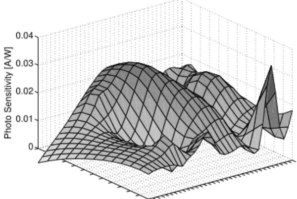
0 0.01 0.02 0.03 0.04
Photo Sensitivity [A/W]
Fig. 2. Signal sample: luminosity in the range320−730nm.
andU(k)are computed from the setX(k), we obtain the vector
of principal componentss(k)inverting (5):
s(k)= (U(k))−1(x(k)−x(k)) = (U(k))T(x(k)−x(k)), (17)
since U(k) is orthonormal by construction and therefore U(k)(U(k))T =I
N.
In what follows we describe the considered signals and the WSN deployment. After that, we present the analysis on the distribution of the elements ofs.
Network: we consider the WSN testbed of Fig. 1. This experimental network is deployed on the ground floor of the Department of Information Engineering at the Univer-sity of Padova. The WSN consists of N = 68 TmoteSky wireless nodes equipped with IEEE 802.15.4 compliant radio transceivers.
Signals: From the above WSN, we gathered five different types of signalsx: S1) humidity, S2-S3) luminosity in two dif-ferent ranges:320−730and320−1100nm, respectively, S4) temperature and S5) battery voltage. We collect measurements from all nodes every5minutes for at least3days. We repeated the data collection for three different measurement campaigns during the month of March 2009, choosing different days of the week: C1) from the13th to the16thof March, C2) from
the19thto the23thand C3) from the24thto the27th. Fig. 2
shows an example signal of type S2, i.e., luminosity in the range320−730 nm.
Principal Component Analysis of Real World Signals:our aim is to infer the statistical distribution of the vector random processs(k)from the samples{s(1),s(2), . . . ,s(T)}which are obtained from the above WSN signals. The parameter T is the duration (number of time samples) of each monitoring campaign C1–C3.
From the theory [6] we know that signals in the PCA domain (in our cases(k)) have in general uncorrelated
compo-nents. Also, in our particular case we experimentally verified that this assumption is good since E[sisj] ≃ E[si]E[sj]
for i, j ∈ {1, . . . , N} and i 6= j. In our analysis, we make a stronger assumption, i.e., we build our model of s
considering statistical independence among its components, i.e., p(si, sj) =p(si)p(sj) with i 6= j, which allows us to
−0.1 −0.05 0 0.05 0.1 Fitting: L Fitting: G Fitting: L0 Fitting: G0
Fig. 3. Empirical distribution and model fitting for a principal component of signal S1, humidity. −0.1 −0.05 0 0.05 0.1 Fitting: L Fitting: G Fitting: L0 Fitting: G0
Fig. 4. Empirical distribution and model fitting for a principal component of signal S2, luminosity in the range320−730nm.
consider the prior (14). A further assumption that we make is to consider the components of s as stationary over the entire monitoring period4. The model developed following this
approach leads to good results [5], which allow us to validate these assumptions.
Owing to these assumptions, the problem of statistically characterizing sreduces to that of characterizing the random variables si= N X j=1 uji(xj−xj), i= 1, . . . , N , (18)
where the r.v. uji is an element of matrix U and the r.v.xj
is an element of vector x.
A statistical model for each si can be determined through
a Bayesian approach (see [13]). For the first level of infer-ence, the observation of the experimental data gives empirical evidence for the selection of four statistical models:
4Note that this assumption does not imply that also the observed processx
is assumed to be stationary. The basisU(k)does not represent a fixed linear
transformation betweenx(k)ands(k), but it changes at each time samplek according to the statistics ofx.
1 3 ... ... N−3 N −510 −210 90 390 690 990 1290 1590
Bayesian Information Criterion, (BIC)
Principal Components, si
BIC: L BIC: G BIC: L0 BIC: G0
Fig. 5. Bayesian Information Criterion (BIC) per Principal Component, for each modelM1–M4, campaign C1 and signal S1, humidity.
M1 a Laplacian distribution with parameters{µ, λ}, that
we call L;
M2 a Gaussian distribution with{m, σ2}, that we callG; M3 a Laplacian distribution with µ= 0 and λ, that we
callL0;
M4 a Gaussian distribution withm= 0andσ2, that we
callG0.
The space of models for eachsi is therefore described by the
set{L,G,L0,G0}. For each signalS1−S5,for each
compo-nentsi, i= 1, . . . , N, and for each model Mi, i= 1, . . . ,4,
we have estimated the parameters (i.e., the most probable
a posteriori, M AP) that best fit the data according to (8).
Since we deal with Gaussian and Laplacian distributions, these estimations have well known and closed form solutions [8]. In detail:
M1 µˆ = µ1/2(s)andˆλ =
PT j=1|sj−µˆ|
T , where µ1/2(s)
is the median of the data; M2 mˆ = PT j=1sj T andσˆ2= PT j=1(sj−mˆ) 2 T−1 ; M3 λˆ= PT j=1|sj| T ; M4 σˆ2= PT j=1s 2 j T .
Figs. 3–4 show two examples of data fitting according to the aforementioned models; in these figures we plot the empirical distribution and the corresponding inferred statistical model for a generic principal component of the humidity (S2) and the luminosity (S4), respectively. From these graphs it is already clear that the distribution of the principal components of our signals is well described by a Laplacian distribution. For the second level of inference we ranked each model according to the Bayesian Information Criterion (BIC) (see Eq. (9)). Fig. 5 shows the BIC for the humidity signal of campaign C1 for all principal components and for all the considered models. From this figure we see that the Laplacian models better fit the data for all principal components si, i= 1,2, . . . , N. The average
BIC for each model, for the different signals and the three campaigns C1–C3, is shown in Table I. The values of this table
Campaign C1 S1 S2 S3 S4 S5 L 1320.2 2481.9 2186.3 1708.5 5374.0 G 1191.7 2226.8 1813.0 1540.1 4139.2 L0 1322.6 2485.0 2189.3 1711.4 5377.3 G0 1194.1 2229.8 1815.9 1542.7 4141.5 Campaign C2 S1 S2 S3 S4 S5 L 921.2 2740.8 2065.4 1483.4 6094.0 G 463.2 1727.7 815.6 749.0 5152.4 L0 924.3 2744.0 2068.8 1486.1 6097.5 G0 466.2 1730.7 818.4 751.9 5155.3 Campaign C3 S1 S2 S3 S4 S5 L 430.3 1207.4 851.3 773.9 3239.7 G 272.9 737.0 301.1 585.8 2676.7 L0 432.7 1210.4 854.4 776.5 3242.9 G0 275.5 739.8 303.8 588.6 2679.3 TABLE I
BAYESIANINFORMATIONCRITERION(BIC)AVERAGED OVER ALL PRINCIPALCOMPONENTS,FOR EACH MODELM1–M4,EXPERIMENTAL
CAMPAIGNSC1–C3AND SIGNALSS1–S5.
are computed averaging over the N principal components. From these results we see that model L0 provides the best
statistical description of the experimental data. In fact, the BIC metric is higher for Laplacian models in all cases; furthermore, L0 has a higher evidence with respect to L, since it implies
the utilization of a single parameter. As previously mentioned, the over-parameterization of the model is penalized according to the factorT−ℓ
2 (see Eq. (9)). Based on the above results we can make the following observations:
1 In our monitoring framework which jointly exploits CS and PCA (Section II), the principal components of real world signals are Laplacian distributed with good approx-imation, therefore it is legitimate to use the prior (14); 2 it is possible to determine, for each principal component,
an optimal parameterλˆ that differs from zero, and there-fore we can exploit (15) with αˆ ←ˆλ;
2.1 in case all principal components are equally distributed with parameter ˆλ, we have that, as demonstrated in Section III, CS obtains the best recovery performance, i.e., at each time k, it finds the s(k) that maximizes the posterior (15);
2.2 in case the principal components are Laplacian distributed with different parameters and these can all be estimated from the data, following a rationale similar to that of Section III we can say that the best recovery performance can be obtained using CS reweighted [15]. We observe that this is often the case in practice, as confirmed by our empirical measurements. We shall note, however, that the correct online estimation of the different parameters is not straightforward. Nevertheless, standard CS still provides very good reconstruction performance as shown in [5].
V. CONCLUSIONS
In this paper we investigated the effectiveness of data re-covery through joint Compressive Sensing (CS) and Principal
Component Analysis (PCA) in Wireless Sensor Networks (WSNs). At first, we framed our recovery scheme into the context of Bayesian theory proving that, under certain assump-tions on the signal statistics, the use of CS is legitimate, and is in fact optimal in terms of recovery performance. Hence, as the main contribution of the paper we have shown that these assumptions hold for real world data, which we gathered from an actual WSN deployment and processed according to our monitoring framework. This allows us to conclude that the use of CS not only is legitimate in our recovery scheme but also makes it possible to obtain very good performance for the considered data sets.
ACKNOWLEDGMENTS
This research has been partially supported by DOCOMO Euro-Labs, Munich, DE.
The authors gratefully thank Dr. Gianluigi Pillonetto, for fruitful and stimulating discussions, and Mr. Nicola Bressan, for providing the sensor measurements.
REFERENCES
[1] D. Donoho, “Compressed sensing,”IEEE Trans. on Information Theory, vol. 52, no. 4, pp. 4036–4048, Apr. 2006.
[2] E. Cand`es and T. Tao, “Near optimal signal recovery from random projections: Universal encoding strategies?”IEEE Trans. on Information Theory, vol. 52, no. 12, pp. 5406–5425, Dec. 2006.
[3] E. Cand`es, J. Romberg, and T. Tao, “Robust uncertainty principles: Exact signal reconstruction from highly incomplete frequency information,”
IEEE Trans. on Information Theory, vol. 52, no. 2, pp. 489–509, Feb. 2006.
[4] J. Haupt, W. Bajwa, M. Rabbat, and R. Nowak, “Compressive Sensing for Networked Data: a Different Approach to Decentralized Compres-sion,” IEEE Signal Processing Magazine, vol. 25, no. 2, pp. 92–101, Mar. 2008.
[5] R. Masiero, G. Quer, D. Munaretto, M. Rossi, J. Widmer, and M. Zorzi, “Data Acquisition through joint Compressive Sensing and Principal Component Analysis,” in IEEE Globecom 2009, Honolulu, Hawaii, USA, Nov.-Dec. 2009.
[6] C. R. Rao, “The Use and Interpretation of Principal Component Analysis in Applied Research,”Sankhya: The Indian Journal of Statistics, vol. 26, pp. 329–358, 1964.
[7] S. Gull, “The Use and Interpretation of Principal Component Analysis in Applied Research,”Maximum Entropy and Bayesian Methods in Science and Engineering, vol. 1, pp. 53–74, 1988.
[8] J. Skilling, Maximum Entropy and Bayesian Methods. Kluwer aca-demic, 1989.
[9] S. Ji, Y. Xue, and L. Carin, “Bayesian Compressive Sensing,” IEEE Trans. on Signal Processing, vol. 56, no. 6, pp. 2346–2356, Jun. 2008. [10] J. Haupt and R. Nowak, “Signal reconstruction from noisy random projections,”IEEE Trans. on Information Theory, vol. 52, no. 9, pp. 4036–4048, Sep. 2006.
[11] G. Quer, R. Masiero, D. Munaretto, M. Rossi, J. Widmer, and M. Zorzi, “On the Interplay Between Routing and Signal Representation for Compressive Sensing in Wireless Sensor Networks,” in Information Theory and Applications Workshop (ITA 2009), San Diego, CA, US, Feb. 2009.
[12] H. Mohimani, M. Babaie-Zadeh, and C. Jutten, “A fast approach for overcomplete sparse decomposition based on smoothed L0 norm,”IEEE Trans. on Signal Processing, 2009, Accepted for publication. [13] D. J. MacKay, “Bayesian Interpolation,”Neural Computation Journal,
vol. 4, no. 3, pp. 415–447, May 1992.
[14] G. Schwarz, “Estimating the Dimension of a Model,”The Annals of Statistics, vol. 6, no. 2, pp. 461–464, 1978.
[15] E. Cand`es, M. B. Wakin, and S. Boyd, “Enhancing Sparsity by Reweightedℓ1 Minimization,”Journal of Fourier Analysis and Appli-cations, vol. 14, pp. 877–905, Dec. 2008.