APPROXIMATION OF FRAME BASED MISSING DATA RECOVERY
JIAN-FENG CAI∗, ZUOWEI SHEN†, AND GUI-BO YE‡
Abstract. Recovering missing data from its partial samples is a fundamental problem in mathematics and it has wide range of applications in image and signal processing. While many such algorithms have been developed recently, there are very few papers available on their error estimations. This paper is to analyze the error of a frame based data recovery approach from random samples. In particular, we estimate the error between the underlying original data and the approximate solution that interpolates (or approximates with an error bound depending on the noise level) the given data that has the minimalℓ1 norm of the canonical frame coefficients among all the possible solutions.
1. Introduction. Recovering missing data from its partial samples is a fundamental problem in math-ematics and it has wide range of applications in image and signal processing. The problem is to recover the underlying image or signal𝒑from its partial observations given by
𝒈[𝑘] =
{
𝒑[𝑘] +𝜽[𝑘], 𝑘∈Λ,
unknown, 𝑘∈Ω∖Λ, (1.1)
where 𝜽 is the error contained in the observed data. Here the set Ω (see also (1.2)) is the domain where the underlying data is defined and Λ is a subset of Ω where we have the observed data. The observed data could be part of sound, images, time-varying measurement values and sensor data. The task is to recover the missing data on Ω∖Λ. There are many methods to deal with this problem under many different settings, e.g., [3,4,10,25,38] for image inpainting, [11,14,15] for matrix completion, [29,55] for regression in machine learning, [8, 9, 20, 23, 24] for framelet-based image deblurring, [41, 45] for surface reconstruction in computer graphics, and [16,22,26] for miscellaneous applications. We forgo to give a detailed survey on this fast developing area and the interested reader should consult the references mentioned above for the details. Instead, the focus of this paper is to establish the approximation properties of a frame based data recovery method.
The settings of (1.1) considered in this paper are as follows. Let
Ω ={𝑘= (𝑘1, . . . , 𝑘𝑑) :𝑘∈ℤ𝑑,0≤𝑘𝑖< 𝑁, 𝑖= 1, . . . , 𝑑}, (1.2)
where𝑁 is a given positive integer. Let
Λ⊂Ω, ∣Λ∣=𝑚, Λ is uniformly randomly drawn from Ω. (1.3)
Define𝜌:=𝑚/∣Ω∣be the density of the known pixels. Then, in (1.1), the observed data𝒈and the error𝜽are given and fixed, although the error𝜽may be viewed as a particular realization of some random variables, e.g., i.i.d. Gaussian noise. Hence, in this setting, the only random variables are Λ, which is uniformly randomly chosen from Ω.
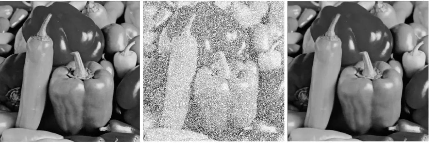
One of the most important examples of our model is image recovery from random sampled pixels, which occurs when part of the pixel is randomly missing due to, e.g., the unliable communication channel [7,26] or the corruption by a salt-and-pepper noise [12, 22]. One of such examples is shown in Figure 1.1. The task of image recovery is to restore the missing region from the incomplete pixels observed. Ideally, the restored image should possess shapes and patterns consistent with the given image in human vision. Therefore, we need to extract information such as edges and textures from the observed data to replace the corrupted part in such a way that it would look natural for human eyes. For this, it is often useful to restore images in a transform domain (e.g. tight frame transform) where the underlying image has a sparse approximation. This leads to a few frame based methods for image restorations as given in e.g. [10,12,38,39].
In this paper, we give the error estimation for a frame based recovery method to solve (1.1)–(1.3). For this, we first introduce the concept of tight frame. See [35, 53] for an overview of tight frame. Letℋ be a
∗Department of Mathematics, University of California, Los Angeles. Email: [email protected]. †Department of Mathematics, National University of Singapore. Email: [email protected]. ‡Department of Computer Science, University of California, Irvine. Email: [email protected].
(a) The 512×512 “peppers” image. (b) 50% pixels are randomly missing. (c) Recovered by (1.8). The algorithm employed is the split Bregman method in [13].
Fig. 1.1: Images
Hilbert space. A sequence{𝒂𝑛}𝑛∈Γ ⊂ ℋis a tight frame ofℋif for an arbitrary element 𝒇 ∈ ℋ
∥𝒇∥2=∑ 𝑛∈Γ ∣⟨𝒇,𝒂𝑛⟩∣2, or, equivalently, 𝒇 =∑ 𝑛∈Γ ⟨𝒇,𝒂𝑛⟩𝒂𝑛. (1.4)
For a given tight frame, the analysis operator𝒜is defined as
𝒜𝒇[𝑛] =⟨𝒇,𝒂𝑛⟩, ∀𝑛∈Γ. (1.5)
The sequence {⟨𝒇,𝒂𝑛⟩}𝑛∈Γ is called the canonical coefficients of the tight frame {𝒂𝑛}𝑛∈Γ. For recovery
problem (1.1) with Ω defined by (1.2), we are working on the finite dimensional space ℋ=ℓ2(Ω). In this case,𝒂𝑛 is a sequence inℓ2(Ω) and Γ is a finite set.
To measure the regularity of the underlying image or signal, one can employ the weighted ℓ1 norm of the canonical frame coefficient. This is commonly used in image and signal processing literature. In this paper, we will use the weightedℓ1 norm of the canonical frame coefficient ∥𝒜𝒇∥ℓ1(𝛽,Υ) for a given𝛽 in the
form of the following
∥𝒜𝒇∥ℓ1(𝛽,Υ)= ∑ 𝑛∈Γ
2𝛽Υ(𝑛)∣⟨𝒂𝑛,𝒇⟩∣, (1.6)
where Υ is a function mapping from Γ toℕsatisfying
max{Υ(𝑛) :𝑛∈Γ} ≤ 1𝑑log2∣Ω∣. (1.7)
Here the parameter𝛽is to control the regularity of𝒇, and the function Υ is to make the weight more flexible so that it allows group weighting. It will be seen in Section 3.1 the usefulness and the explicit form of Υ in the case of framelet. As we know, signals and images are usually modeled by discontinuous functions, and the discontinuity possesses important information. Therefore, our assumption for𝛽 is always small in order to reflect the low regularity of the underlying signal. That is, we are only interested in signals of low regularity in this paper.
The focus of this paper is to study one of the analysis based approach using tight frame. We assume𝒑 satisfies∥𝒜𝒑∥ℓ1(𝛽,Υ)<∞and∥𝒑∥∞≤𝑀, where𝑀 is a given constant. The first condition is the regularity of𝒑and the second condition is the boundedness of each pixel of𝒑. In our model, the approximate solution 𝒇Λ of the problem (1.1) is defined by:
𝒇Λ= arg min{∥𝒜𝒇∥ ℓ1(𝛽,Υ): ∣Λ∣1 ∑ 𝑘∈Λ (𝒇[𝑘]−𝒈[𝑘])2≤𝜎2, ∥𝒇∥ ∞≤𝑀 } . (1.8)
It is clear that there exists at least one solution for the above minimization problem. Indeed, this follows from the facts that the constraint set {f : 1
∣Λ∣
∑
𝑘∈Λ(f[𝑘]−g[𝑘])2 ≤𝜎2,∥f∥∞ ≤𝑀} is closed and bounded and the objective function ∥𝒜f∥ℓ1(𝛽,Υ) is continuous with respect to f. Therefore, 𝒇Λ is well defined and
has a minimal weighted ℓ1 norm of the canonical coefficient subject to reasonable constraints. Here, the
constraint 1
∣Λ∣
∑
𝑘∈Λ(𝒇[𝑘]−𝒈[𝑘])2≤𝜎2is a data fitting term to (1.1) and𝜎2is the error bound. Therefore,𝒑
naturally satisfies this constraint. The constraint∥𝒇∥∞≤𝑀 is to ensure that the recovered signal values are bounded by a preassigned number𝑀. This constraint is usually inactive, i.e., solving (1.8) with or without this constraint gives the same solution in most numerical simulations as long as the original signal 𝒑 also satisfies this constraint. When 𝑚=∣Ω∣ and 𝜎= 0, the unique solution of (1.8) is the original solution 𝒑. Therefore, we are interested in the case when 𝑚 < ∣Ω∣and 𝜎 ∕= 0. In figure 1.1, we give an example that shows (1.8) recovers the missing pixels of the image very well (the algorithm employed for solving (1.8) is the split Bregman method in [13]). The purpose of this paper is to show analytically that the errors of the recovered missing pixels are within the measurement error bound of the given pixels.
As for the energy ∥𝒜𝒇∥ℓ1(𝛽,Υ) in (1.8), at top of the fact that it connects to the regularity of the
underlying function where the data comes from, it can be interpreted as follows that links to the prior distribution of𝒇. In fact, we implicitly assume that the prior distribution of𝒇 satisfying
Prob{𝒇}=𝐶𝑜𝑛𝑠𝑡⋅exp
{
−𝜆∥𝒜𝒇∥ℓ1(𝛽,Υ) }
.
Hence, minimizing∥𝒜𝒇∥ℓ1(𝛽,Υ) is equivalent to maximizing the probability that the data occurs.
An efficient frame based algorithm is developed for some applications to solve (1.8) in [13]. The algorithm is implicitly based on the fact that 𝒇 has a sparse approximation under the tight frame system used. A sparse approximation means majority of the canonical coefficients 𝒜𝒇 are small and negligible. In this sense, (1.8) gives a sparse approximate solution of (1.1). However, there are big differences between the approach (1.8) here and compressed sensing (see e.g. [16–18,32]) — one of the hottest research topics based on sparsity. Firstly, the requirement of sparsity here is much weaker than in compressed sensing. We do not require explicitly the sparsity of either𝒇 or its canonical frame coefficient. Instead, we assume the decay of the canonical frame coefficient in the sense that the weightedℓ1 norm (1.6) is bounded. Secondly, in basis pursuit of compressed sensing, the signal is synthesized by a sparse coefficient, hence it is a synthesis based approach. However, as mentioned before, the model (1.8) is an analysis based approach — the analyzed coefficient has a sparse approximation. There is a gap between the analysis and synthesis based approaches as pointed out in, e.g., [13, 37]. Last and most importantly, the matrix here does not satisfy the restricted isometry property (RIP) required in the theoretic analysis in compressed sensing. If we use a synthesis based approach instead of the analysis based approach (1.8), then the sensing matrix will be 𝒫Λ𝒜𝑇, where𝒫Λ is
an operator satisfying𝒫Λ𝒇[𝑘] =𝒇[𝑘] for 𝑘∈Λ and𝒫Λ𝒇[𝑘] = 0 for 𝑘∈Ω∖Λ. Since usually each vector 𝒂𝑖
(each row of𝒜) is locally supported, by a simple calculation, one finds that𝒫Λ𝒜𝑇 has at least one column
being the zero vector with a high probability. In turn, the sensing matrix does not satisfy the RIP with high probability. The matrix 𝒫Λ does not satisfy the concentration inequality in [52]. Moreover, due to
the compact support property of the frame elements𝒂𝑖, the incoherence conditions (see [33] for instance)
between the column vectors of matrix 𝒫Λ and the row vectors of 𝒜may not hold. This causes that there
contains no enough information in the observed pixels for exact signal recovery. Therefore, the compressed sensing theory cannot be applied here, even the synthesis based approach is used.
This paper is to bound the error between the underlying unknown data𝒑and the approximate solution 𝒇Λ given by (1.8). It is clear that one can only expect that the recovered error is within the level of the
measurement error up to a constant. It is trivially true when the density𝜌= 1 (i.e., Λ = Ω), since 1 ∣Ω∣ ∑ 𝑘∈Ω (𝒇Λ[𝑘]−𝒑[𝑘])2≤ 2 ∣Ω∣ ∑ 𝑘∈Ω (𝒇Λ[𝑘]−𝒈[𝑘])2+ 2 ∣Ω∣ ∑ 𝑘∈Ω (𝒈[𝑘]−𝒑[𝑘])2≤4𝜎2.
We are interested to know what will happen when the density 𝜌 < 1. In fact, we will show that, under some mild assumptions, with probability 1−𝛿for an arbitrary fixed𝛿∈(0,1), the error between𝒑and𝒇Λ
satisfies 1 ∣Ω∣∥𝒇Λ−𝒑∥2ℓ2(Ω)≤𝐶𝜌− 1 2√log2∣Ω∣(∣Ω∣)−𝑏log1 𝛿 + 16 3 𝜎2, (1.9)
where 𝑏 is a positive constant and will be given explicitly in Theorem 2.2, and 𝐶 is a positive constant independent of𝜌,∣Ω∣, 𝛿 or𝜎when the tight framelets are used . Roughly, it says that as long as the data set is sufficiently large, one has a pretty good chance to recover the original data within the measurement error bound by solving (1.8).
The main difficulty here is that the underlying solution has a low regularity. The analysis here is based on the combination of the uniform law of large numbers, which is standard in classical empirical processes and statistical learning theory, and an estimation for its involved covering number. The covering number estimation given here is new involved, since the standard estimation for it is too large so that it is not good enough to derive the desired convergence rate. Our estimation for the covering number uses the special structure of the set and the max-flow min-cut theorem in graph theory. The error analysis here can be easily extended into more analysis based approaches, e.g. total variation method for imaging restorations.
The paper is organized as follows. In Section 2, we give our main results of approximation analysis for the frame based signal recovery method (1.8). Error estimations are given. Then, in Section 3, an application of our main results is illustrated. More precisely, we estimate the error of framelet based image recovery algorithms from random samples. Based on this, we further link the discrete approximation of solution to the function approximation of it in the content of multiresolution analysis and its associated tight frammlets given by [51]. Finally, the technical proofs of the critical lemmas and theorems are given in Section 4.
2. Error Analysis. In this section, we give the error analysis of the model (1.8) for a given tight frame analysis operator𝒜. That is, we study the asymptotic property of∥𝒇Λ−𝒑∥ℓ2(Ω)with respect to∣Ω∣. Here Λ
is a data set with each element i.i.d drawn from uniform distribution of Ω and∣Ω∣denotes the cardinality of the set Ω. Such problem is well known in classical empirical processes [54] and statistical learning theory [55]. The most powerful tool used there is the uniform law of large numbers and our analysis is along this direction. To employ the uniform law of large numbers, the key issue is the capacity of the involved set. There are many tools to characterize the capacity of a set in the literature, e.g. 𝑉 𝐶-dimension [55], 𝑉𝛾-dimension,
𝑃𝛾-dimension [1], Rademacher complexities [2,46] and covering number [29]. As covering number is the most convenient and very powerful for metric space, we choose it to characterize the capacity of the involved set
ℳ={𝒇 ∈ℓ∞(Ω) :∥𝒜𝒇∥ℓ1(𝛽,Υ)≤ ∥𝒜𝒑∥ℓ1(𝛽,Υ),∣Λ∣1 ∑ 𝑘∈Λ (𝒇[𝑘]−𝒈[𝑘])2≤𝜎2, ∥𝒇∥ ∞≤𝑀 } . (2.1)
Here, the constants𝑀 and𝜎are fixed. Notice that, with high probability, the underlying true solution𝒑is in the setℳ. Furthermore, according to the definition of 𝒇Λ by (1.8), we have∥𝒜𝒇Λ∥ℓ1(𝛽,Υ)≤ ∥𝒜𝒑∥ℓ1(𝛽,Υ)
and obviously𝒇Λ∈ ℳ. Thus, the setℳdefined in (2.1) is the set we concerned.
To further illustrate our idea, we give the concept of the covering number, which is adapted to the settings of this paper.
Definition 2.1. Let ℳ ⊂ℝ∣Ω∣ and 𝜂 >0 be given. Thecovering number 𝒩(ℳ, 𝜂)is the minimal number of the ℓ∞ balls with radius𝜂 inℳ that coverℳ.
The main difficulty of this paper is to give a tight estimate of the covering number𝒩(ℳ, 𝜂) of the set ℳ defined in (2.1). At first glance,ℳ is a subset of{𝒇 ∈ℓ∞(Ω) :∥𝒇∥∞≤𝑀
}
, which is a ball in finite dimensional Banach spaceℓ∞(Ω). We have a simple bound for the covering number of this set, that is,
𝒩(ℳ, 𝜂)≤ ( 𝑀 𝜂 )∣Ω∣ , (2.2)
see the details in [29]. However, this estimation is not tight enough to derive a convergence rate of the error ∥𝒇Λ−𝒑∥ℓ2(Ω). We need to find a much tighter bound of 𝒩(ℳ, 𝜂) by further exploiting the conditions of
the setℳ. As mentioned before,∥𝒜𝒇∥ℓ1(𝛽,Υ)is a measure of regularity of𝒇, it is reasonable to get a much
tighter bound by exploiting the condition ∥𝒜𝒇∥ℓ1(𝛽,Υ)≤ ∥𝒜𝒑∥ℓ1(𝛽,Υ). However, things are becoming more
complicated as this regularity condition is quite low from the functional point of view and any known results can not help us to achieve desired results. If we view the condition ∥𝒜𝒇∥ℓ1(𝛽,Υ) ≤ ∥𝒜𝒑∥ℓ1(𝛽,Υ) discretely
and not connect it to its underlying function, it is too complicated to analyze because of the complicated structure of the frame operator 𝒜. This motivates us to assume that the tight frame system 𝒜 in (1.8) satisfy a mild regularity property — the discrete total variation has to be small. More specifically, we first give the definition of the discrete difference operator𝒟. For any𝒇 ∈ℓ∞(Ω), we define
𝒟𝒇 ={𝒇[𝑘1, . . . , 𝑘𝑖−1, 𝑘𝑖+ 1, 𝑘𝑖+1. . . , 𝑘𝑑]−𝒇[𝑘1, . . . , 𝑘𝑑]}1≤𝑖≤𝑑,(𝑘1,...,𝑘𝑑),(𝑘1,...,𝑘𝑖+1...,𝑘𝑑)∈Ω. (2.3) From the constraints 1≤𝑖≤𝑑,(𝑘1, . . . , 𝑘𝑑),(𝑘1, . . . , 𝑘𝑖+ 1. . . , 𝑘𝑑)∈Ω, we know that𝒟𝒇 is a vector with total number of𝑑(∣Ω∣ − ∣Ω∣𝑑−𝑑1) entries. Theℓ1norm of vector𝒟𝒇 is
∥𝒟𝒇∥1= 𝑑 ∑ 𝑖=1 ∑ (𝑘1, . . . , 𝑘𝑑)∈Ω, (𝑘1, . . . , 𝑘𝑖+ 1. . . , 𝑘𝑑)∈Ω ∣𝒇[𝑘1, . . . , 𝑘𝑖−1, 𝑘𝑖+ 1, 𝑘𝑖+1. . . , 𝑘𝑑]−𝒇[𝑘1, . . . , 𝑘𝑑]∣. (2.4)
We call∥𝒟𝒇∥1 a discrete total variation. In particular, when𝑑= 2, it becomes
∥𝒟𝒇∥1= ∑ (𝑘1, 𝑘2)∈Ω (𝑘1 + 1, 𝑘2)∈Ω ∣𝒇[𝑘1+ 1, 𝑘2]−𝒇[𝑘1, 𝑘2]∣+ ∑ (𝑘1, 𝑘2)∈Ω (𝑘1, 𝑘2 + 1)∈Ω ∣𝒇[𝑘1, 𝑘2+ 1]−𝒇[𝑘1, 𝑘2]∣.
For a given frame system{𝒂𝑛}𝑛∈Γ ofℓ2(Ω), we say that it satisfies the bounded condition of the discrete
total variation if there exists a positive constant𝐶𝑑 such that
∥𝒟𝒂𝑛∥1≤𝐶𝑑2𝛼Υ(𝑛), 𝑛∈Γ, 𝛼≤𝑑−1, (2.5)
where Υ is defined by (1.7). This condition links to the regularity of tight frame systems and most tight frame systems satisfy (2.5) with certain𝛼. This condition is also verifiable in many cases, and straightforward sometimes.
Under the condition (2.5), we can relax the setℳto the set
˜
ℳ={𝒇 ∈ℓ∞(Ω) :∥𝒟𝒇∥1≤𝐶𝑑∣Ω∣
max{𝛼−𝛽,0}
𝑑 ∥𝒜𝒑∥ℓ1(𝛽,𝛾),∥𝒇∥∞≤𝑀} (2.6)
by simple calculation andℳ ⊂ℳ. Then we exploit the features of the set˜ ℳ˜and use the famous max-flow min-cut in graph theory to derive the desired estimate of the covering numbers, see Section 4 for more details.
With all these notations, we can give the explicit form of our main result.
Theorem 2.2. Let 𝒇Λ be defined as (1.8), and 𝒜 as (1.5). Assume that the frame {𝒂
𝑛}𝑛∈Γ satisfies
(2.5) and∥𝒜𝒑∥ℓ1(𝛽,Υ) ≤𝐶𝒑∣Ω∣12 with 𝛼−𝑑
2 ≤𝛽 ≤𝛼+𝑑2. Then for an arbitrary 0 < 𝛿 <1, the following
inequality
1
∣Ω∣∥𝒇Λ−𝒑∥2ℓ2(Ω)≤˜𝑐𝜌− 1
2∣Ω∣−min{𝑑+2(4𝛽−𝛼𝑑 ),14}√log2∣Ω∣log1 𝛿+ 16 3 𝜎2, where˜𝑐=256 3 𝑀2+ 32𝑀 √
𝑀(2𝑀+ 2(𝑑+ 1)𝐶𝑑𝐶𝒑), holds with confidence1−𝛿.
Note that the condition used in this theorem is quite general and only some low regularity condition for the frame 𝒜and original data𝒑 is required. The results is exciting as mentioned in the introduction. For fixed𝜌, as long as the cardinality of Ω is large enough,𝒇Λ gives a good approximation of the original data𝒑.
Furthermore, for fixed Ω, if we let 𝜌become larger, then we can get smaller error. This result is consistent with our common sense as we are given more data for fixed Ω with larger𝜌.
In the following, we prove Theorem 2.2 — the main theorem of this paper. Following the same line as the technique used in statistical learning theory [55], instead of estimating the error 1
∣Ω∣∥𝒇Λ−𝒑∥2ℓ2(Ω)
directly, we first calculate the probability that the error 1
∣Ω∣∥𝒇Λ−𝒑∥2ℓ2(Ω) is smaller than a fixed number by
using the theorem of uniform law of large numbers. This leads to the following theorem, which estimates the probability of event 1
∣Ω∣∥𝒇Λ−𝒑∥2ℓ2(Ω) ≤𝜖+163𝜎2 for an arbitrary given 𝜖in terms of the covering numbers
with its radius related to𝜖. We leave the proof in Section 4.
Theorem 2.3. Let ℳ be defined by (2.1) and 𝒇Λ by (1.8). Then for an arbitrary given 𝜖 > 0, the
inequality Prob { 1 ∣Ω∣∥𝒇Λ−𝒑∥2ℓ2(Ω)≤𝜖+163 𝜎2 } ≥1− 𝒩(ℳ,12𝜖𝑀) exp { −2563𝑚𝜖𝑀2 }
holds for an arbitrary𝑚, where𝑚 is the number of samples. Proof. See Section 4.1.
In order to give the explicit convergence rate of ∥𝒇Λ−𝒑∥ℓ2(Ω), we need an explicit estimate of the
covering number 𝒩(ℳ, 𝜂). The following theorem concerns an upper bound of 𝒩(ℳ, 𝜂). As its proof is too complicated, we leave it in Section 4 for the reader more easy to understand the idea of this paper. The main difficulty we overcome is the low regularity of the sequence in the setℳas 𝛽 is not large enough here. We overcome it by using the powerful tool of discrete total variation and max-flow min-cut theorem. It should be noted that only discrete total variation is used to measure the regularity of the sequence inℳ for covering number estimation, so our analysis is still true for more general case such as similar𝑇 𝑉 based algorithms, see Section 4 for more details.
Theorem 2.4. Let ℳ be defined as (2.1) and 𝒜 as (1.5). Assume that the frame {𝒂𝑛}𝑛∈Γ satisfies
(2.5)and∥𝒜𝒑∥ℓ1(𝛽,Υ)≤𝐶𝒑∣Ω∣12 with 𝛽≤𝛼+𝑑
2, then for any𝜂≥ ∣Ω∣max{ 𝑑+2(𝛼−𝛽) 2𝑑 ,12}−1, log𝒩(ℳ, 𝜂)≤𝐶𝑑′∣Ω∣max{ 𝑑+2(𝛼−𝛽) 2𝑑 ,12}log2∣Ω∣ 𝜂 , where𝐶′ 𝑑= 2𝑀 + 2(𝑑+ 1)𝐶𝑑𝐶𝒑.
Proof. See Section 4.2.
With all of these, we are now ready to prove Theorem 2.2. The technique used for the proof is somewhat similar to the one used in statistical learning theory [29]. The main difference is that we have some constraint for𝜂 in our bound for covering number given in Theorem 2.4, so we need to verify that this constraint will not influence the proof of Theorem 2.2.
Proof of Theorem 2.2. First, by Theorem 2.3, for an arbitrary given𝜖≥12𝑀∣Ω∣max{𝑑+2(2𝛼−𝛽𝑑 ),12}−1,
and𝜂= 𝜖
12𝑀 the inequality
1
∣Ω∣∥𝒇Λ−𝒑∥2ℓ2(Ω)≤𝜖+163 𝜎2
holds with the confidence at least
1− 𝒩(ℳ,12𝜖𝑀) exp { −2563𝑚𝜖𝑀2 } ≥1−exp { 12𝑀𝐶′ 𝑑∣Ω∣max{ 𝑑+2(𝛼−𝛽) 2𝑑 ,12}log2∣Ω∣ 𝜖 } exp { − 3𝑚𝜖 256𝑀2 } .
The last inequality follows from Theorem 2.4. Next, choosing a special𝜖∗to be the unique positive solution of the following equation
12𝑀𝐶′ 𝑑∣Ω∣max{ 𝑑+2(𝛼−𝛽) 2𝑑 ,12}log2∣Ω∣ 𝜖 − 3𝑚𝜖 256𝑀2 = log𝛿, (2.7)
we have 1
∣Ω∣∥𝒇Λ−𝒑∥2ℓ2(Ω)≤𝜖∗+163𝜎2with confidence 1−𝛿if we can prove that𝜖∗≥12𝑀∣Ω∣max{ 𝑑+2(𝛽−𝛼)
2𝑑 ,12}−1.
However, solving the equation (2.7) yields
𝜖∗=32𝑀 3𝑚 ( 4𝑀log1𝛿 + √ 16𝑀2log21 𝛿 + 9𝑚𝑀𝐶𝑑′∣Ω∣max{ 𝑑+2(𝛼−𝛽) 2𝑑 ,12}log2∣Ω∣ ) (2.8) ≤323𝑚𝑀 ( 8𝑀log1𝛿+ 3 √ 𝑚𝑀𝐶′ 𝑑∣Ω∣max{ 𝑑+2(𝛼−𝛽) 2𝑑 ,12}log2∣Ω∣ ) ≤˜𝑐𝜌−1
2√log2∣Ω∣∣Ω∣−min{𝑑+2(4𝛽−𝛼𝑑 ),14}log1 𝛿,
where˜𝑐=256
3 𝑀2+ 32𝑀 √
𝑀𝐶′
𝑑. Also, from (2.8), we know that 𝜖∗≥ 32√𝑀 𝑚 √ 𝑀𝐶′ 𝑑∣Ω∣max{ 𝑑+2(𝛼−𝛽) 2𝑑 ,12}log2∣Ω∣ ≥16𝑀 √ 𝑀𝐶′ 𝑑𝜌− 1 2√log 2∣Ω∣∣Ω∣max{ 𝑑+2(𝛼−𝛽) 4𝑑 ,14}−12,
which implies that𝜖∗≥12𝑀∣Ω∣max{𝑑+2(𝛼−𝛽)
2𝑑 ,12}−1. This concludes the proof.
3. Image Recovery from Random Samples by Framelet. Before going to the proofs of the tech-nical theorems in the previous section, we apply Theorem 2.2 to framelet based image recovery from random samples in this section. Various algorithms of framelet based image recovery algorithms have been developed in [9, 10, 13, 38, 39]. Especially, an efficient algorithm for framelet based image recovery by using splitting Bregman iteration is given in [13]. For this framelet based image recovery algorithm, we are able to link the approximation property of the algorithm to the regularity of the underlying function (in terms of the decay of its canonical coefficients of given tight frames) where the pixels come from. We start with discussions of the approximation of the framelet based recovery. It is then followed by the link of this analysis to the functional space. We restrict our discussions here for two variable functions, since the images can be viewed as a set of data sampled from two variable functions. For more general multi-variable functions, the discussions are the same.
3.1. Framelet. A wavelet (or affine) system 𝑋(Ψ, 𝜙) derived from the multiresolution analysis gener-ated by a refinable function 𝜙is defined to be the collection of dilations and shifts of a finite set Ψ ={𝜓ℓ: ℓ= 1,2, . . . , 𝐿} ⊂𝐿2(ℝ2), i. e.,
𝑋(Ψ, 𝜙) ={𝜓ℓ
𝑗,𝑘:= 2𝑗𝜓ℓ(2𝑗𝑥−𝑘) :𝑗∈ℤ, 𝑘∈ℤ2, ℓ= 1,2, . . . , 𝐿}.
The elements in Ψ are called the generators. When 𝑋(Ψ, 𝜙) is also a tight frame for 𝐿2(ℝ2), then 𝜓∈Ψ
are called(tight) framelets, following the terminology used in [31]. Recall that 𝑋(Ψ, 𝜙) is a tight frame for
𝐿2(ℝ2) if, for any𝑓 ∈𝐿2(ℝ2),
𝑓 = 𝐿 ∑ ℓ=1 ∑ 𝑗∈ℤ ∑ 𝑘∈ℤ2 ⟨𝑓, 𝜓ℓ 𝑗,𝑘⟩𝜓𝑗,𝑘ℓ .
To construct compactly supported framelet systems, one starts with a compactly supported refinable function𝜙∈𝐿2(ℝ2) with a refinement mask (low-pass filter)𝒉
0such that𝜙satisfies the refinement equation: 𝜙(𝑥) = 4∑
𝑘
𝒉0[𝑘]𝜙(2𝑥−𝑘). (3.1)
Let𝑉0be the closed shift invariant space generated by{𝜙(⋅ −𝑘) :𝑘∈ℤ2}and𝑉𝑗 :={𝑓(2𝑗⋅) :𝑓 ∈𝑉0, 𝑗∈ℤ}.
It is known that when 𝜙 is compactly supported, the sequence {𝑉𝑗}𝑗∈ℤ forms a multiresolution analysis. Recall that{𝑉𝑗}𝑗∈ℤ is said to generate a multiresolution analysis (MRA) if (a)𝑉𝑗 ⊂𝑉𝑗+1, (b)∪𝑗𝑉𝑗 is dense
in𝐿2(ℝ2), (c)∩𝑗𝑉𝑗={0}, see [44,51] for more details.
In this paper, we assume that the refinable function𝜙satisfy the following conditions: Assumption 1.
(a) 𝜙:ℝ27→ℝ2 is compactly supported with∫𝜙= 1.
(b) 𝜙 is H¨older continuous with exponent 1, i.e. there exists a constant 𝐶˜ such that for any 𝑥, 𝑦 ∈
ℝ2,∣𝜙(𝑥)−𝜙(𝑦)∣ ≤𝐶˜∥𝑥−𝑦∥, where∥ ⋅ ∥is the Euclidean norm in ℝ2.
(c) {𝜙(⋅ −𝑘)}𝑘∈ℤ2 is a Riesz Basis in the space𝑉0.
There are many refinable functions satisfy the above assumptions, e.g. the tensor product pseudo splines (see e.g. [31, 34], or simply three directional box splines see e.g. [5]). The Riesz basis requirement is not so crucial. For example, it is not required in applying the unitary extension principle for the construction of tight framelets.
The compactly supported frameletsΨ are defined by
𝜓ℓ(𝑥) = 4∑ 𝑘
𝒉ℓ[𝑘]𝜙(2𝑥−𝑘)
for some compactly supported sequence𝒉ℓinℓ∞(ℤ2). When the filters{𝒉𝑖, 𝑖= 0, . . . , 𝐿}satisfy the following conditions 𝐿 ∑ ℓ=0 ∣ˆ𝒉ℓ(𝜔)∣2= 1 and 𝐿 ∑ ℓ=0 ˆ 𝒉ℓ(𝜔)ˆ𝒉ℓ(𝜔+𝜋) = 0, a.e. 𝜔∈[−𝜋, 𝜋], (3.2)
where𝒉ˆℓ(𝜔) :=∑𝑘∈ℤ2𝒉ℓ[𝑘]𝑒−𝑖𝑘𝜔, then the wavelet system𝑋(Ψ, 𝜙) is a tight wavelet frame by the unitary
extension principle (UEP) in [51]. The corresponding mask𝒉0is refinement mask which is a low pass filter
and{𝒉ℓ: 1≤ℓ≤𝐿}are framelet masks which are high pass filters. Since the publication of UEP [51] and
oblique extension principle (OEP) of [28] and [31], there are many construction of framelets using UEP and OEP, see [27,47, 50] and references therein.
The advantage of framelet is that the discrete tight frame system for the computation is easy to derive by framelet decomposition and reconstruction algorithms of [31]. First, we construct
˜ 𝒂0= 2𝐽𝒉|0∗ ↑. . .{z 𝒉0∗ ↑} 𝐽 𝜹 (3.3) and ˜𝒃ℓ 𝑗 = 2𝐽−𝑗𝒉|0∗. . .{z↑𝒉0∗ ↑} 𝐽−𝑗−1 𝒉ℓ∗ ↑𝜹, (3.4)
where 𝜹is a sequence with each component 𝜹[𝑘] = 1 when 𝑘= (0,0) and𝜹[𝑘] = 0 otherwise, and𝒉0∗ ↑is
an upsampling operator, i.e., for a sequence𝒄∈ℓ2(ℤ2),
𝒉0∗ ↑c= ∑
𝑘
𝒉0[𝑛−2𝑘]𝒄[𝑘].
Using these sequences, one can derive the standard framelet decomposition algorithm as suggested in [31]. Let𝒇 ∈ℓ2(Ω) be an image with
Ω ={𝑘= (𝑘1, 𝑘2) : 0≤𝑘1, 𝑘2<2𝐽}. (3.5)
To make a suitable tight frame analysis, one needs to impose proper boundary conditions. Periodic boundary conditions are imposed here. We still useℓ2(Ω) to denote the space of sequences defined onℓ2(Ω) with periodic boundary conditions. Other boundary conditions can be discussed similarly, we forgo the discussion here and the interested reader should consult [8,23] for more details. Let𝒫 be an operator that maps a vector in
ℓ2(ℤ2) intoℓ2(Ω)
𝒫(𝒗)[𝑘] = ∑
𝑘′ 1,𝑘′2∈ℤ
Let
𝒂0=𝒫(˜𝒂0) (3.6)
and
𝒃ℓ,𝑘𝑗 =𝒫(˜𝒃ℓ
𝑗[⋅ −𝑘]), (3.7)
where ˜𝒂0 is defined by (3.3) and˜𝒃ℓ𝑗 by (3.4). Then, the sequence {𝒂0} ∪ {𝒃𝑗𝑘,ℓ}0≤𝑘1,𝑘2<2𝑗,0≤𝑗<𝐽,1≤ℓ≤𝐿 is a
tight frame system for the spaceℓ2(Ω) with periodic boundary condition by the tight framelet theory (see e.g. [20]). With this tight frame system, the analysis operator𝒜is defined as
∀𝒇, 𝒜𝒇 ={{⟨𝒂0,𝒇⟩}, {⟨𝒃ℓ,𝑘𝑗 ,𝒇⟩ }
0≤𝑘1,𝑘2<2𝑗,0≤𝑗<𝐽,1≤ℓ≤𝐿 }
. (3.8)
Denote the adjoint of𝒜by𝒜∗. By the fact that filters{h
𝑖}𝐿𝑖=0 form a tight frame system, we have
𝒇 =𝒜∗𝒜𝒇 =⟨𝒂0,𝒇⟩𝒂 0+ 𝐽−1 ∑ 𝑗=0 2𝑗−1 ∑ 𝑘1,𝑘2=0 𝐿 ∑ ℓ=1 ⟨𝒃ℓ,𝑘𝑗 ,𝒇⟩𝒃ℓ,𝑘𝑗 . (3.9)
The operator 𝒜∗ is also called synthesis operator. Once we have the analysis operator 𝒜, we define the weighted norm∥𝒜𝒇∥ℓ1(𝛽) for a given𝛽 by
∥𝒜𝒇∥ℓ1(𝛽)=∣⟨𝒂0,𝒇⟩∣+ ∑ 0≤𝑗<𝐽 2𝑗𝛽∑ 𝑘,ℓ ∣⟨𝒃ℓ,𝑘𝑗 ,𝒇⟩∣. (3.10)
Note that the tight frame system {𝒂0} ∪ {𝒃𝑘,ℓ𝑗 }0≤𝑘1,𝑘2<2𝑗,0≤𝑗<𝐽,1≤ℓ≤𝐿 is indexed by (𝑗, 𝑘, ℓ), where 𝑘 =
(𝑘1, 𝑘2)∈ℤ2. The same weight is used for the same subscript𝑗 in the above definition of∥𝒜𝒇∥ℓ1(𝛽). More
explicitly, using the notation in (1.6), we have chosen Γ = {0} ∪ {(𝑗, 𝑘, ℓ) : 0≤𝑘1, 𝑘2 <2𝑗,0≤𝑗 < 𝐽,1≤ ℓ≤𝐿} and the sequence Υ is defined as
Υ(0) = 0, and Υ(𝑗, 𝑘, ℓ) =𝑗.
Since𝑗 < 𝐽 := 1
2log2∣22𝐽∣,the condition (1.7) naturally holds under this definition of Υ.
This weighted norm (3.10) links to regularity of the underlying function where the pixel𝒇 derived from, see [6, 40, 49] and Section 3.3 for more discussions.
3.2. Approximation by Framelet. Let𝒑be a given sequence defined onℓ2(Ω) satisfying∥𝒜𝒑∥ℓ1(𝛽)<
∞and∥𝒑∥∞≤𝑀 for some preassigned constants𝛽 and𝑀. Then, the approximation solution𝒇Λ defined by (1.8) becomes 𝒇Λ= arg min{∥𝒜𝒇∥ ℓ1(𝛽): ∣Λ∣1 ∑ 𝑘∈Λ (𝒇[𝑘]−𝒈[𝑘])2≤𝜎2,∥𝒇∥ ∞≤𝑀 } . (3.11)
This section gives an error analysis for 1
22𝐽∥𝒇Λ−𝒑∥2ℓ2(Ω) for the framelet based image recovery. To apply
Theorem 2.2, we only need to verify (2.5). In fact, we have the following lemma which states that the condition (2.5) is satisfied with𝛼= 0 for𝒜derived from𝑋(Ψ, 𝜙) satisfying Assumption 1.
Lemma 3.1. Assume that refinable function𝜙satisfies Assumption 1. Let 𝒜be defined as (3.8)by the compactly supported tight framelet system 𝑋(Ψ, 𝜙)with compactly supported high-low filters derived by the unitary extension principle from the refinable function𝜙. Then
max{∥𝒟𝒂0∥1,sup 𝑗,ℓ ∥𝒟𝒃
ℓ,𝑘
𝑗 ∥1} ≤𝐶𝑑 (3.12)
for some constant 𝐶𝑑≥1, which is independent of𝐽. Furthermore, for each𝒇 ∈ ℳ, we have
Proof. See Section 4.3.
Using Theorem 2.3 and Lemma 3.1, we can easily derive the following corollary.
Corollary 3.2. Let 𝒜 be defined as (3.8)by the compactly supported tight framelet system 𝑋(Ψ, 𝜙) with compactly supported high-low filters derived by the unitary extension principle from refinable function𝜙
that satisfies Assumption 1. Let𝒇Λ be defined in (3.11). Assume that ∥𝒜𝒑∥
ℓ1(𝛽)≤𝐶𝒑2𝐽 and−1< 𝛽 <1.
Then for any0< 𝛿 <1, with confidence 1−𝛿, 1 22𝐽∥𝒇Λ−𝒑∥2ℓ2(Ω)≤˜𝑐𝜌− 1 2√𝐽2−𝐽min{1+2𝛽,12}log1 𝛿+ 16 3 𝜎2, where˜𝑐=256 3 𝑀2+ 32𝑀 √ 𝑀(2𝑀+ 6𝐶𝑑𝐶𝒑).
Proof. By applying lemma 3.1, we know that the condition (2.5) satisfies with𝛼= 0. Then the corollary can be deduced directly from Theorem 2.2 by letting∣Ω∣= 22𝐽 and𝛼= 0.
3.3. Connection to Function Approximation. This section is to link the estimate given before to the function approximation if we assume that the data is obtained by sampling a function which converts analog signal to digital signal. For example, for the image, the pixels are well modeled by local weighted averages of some underlying function 𝑝 that closely fits the physics of CCD cameras. Furthermore, the pixel values of an image can be viewed as the inner product of𝑝and some refinable function without much loss [21]. More specifically, let 𝜙be a refinable function satisfying∫ 𝜙= 1, and denote the scaled functions by𝜙𝐽,𝑘:= 2𝐽𝜙(2𝐽⋅ −𝑘) for𝑘∈Ω. Then, each pixel value is obtained by
𝒑[𝑘] = 2𝐽⟨𝑝, 𝜙𝐽,𝑘⟩, 𝑘∈Ω. (3.14)
With𝒑[𝑘], implicitly, we use function
𝑝𝐽= ∑ 𝑘∈Ω 𝒑[𝑘]𝜙(2𝐽⋅ −𝑘) =∑ 𝑘∈Ω ⟨𝑝, 𝜙𝐽,𝑘⟩𝜙𝐽,𝑘
to approximate𝑝. The approximation order of𝑝𝐽 to𝑝has been studied extensively. Roughly, as long as𝜙
meets the Strang and Fix condition of a certain order and the Fourier transform of𝜙is flat enough at the origin, then𝑝𝐽will have a good approximation to𝑝. For example, assume that𝜙satisfies the Strang and Fix condition with certain order, and 1− ∣𝜙ˆ(0)∣2has the same order of zeros, where ˆ𝜙is the Fourier transform of 𝜙, and𝑝is sufficiently smooth, then𝑝𝐽 provides this order of approximation to𝑝. Interested reader should consult [31] for details. However, this requires the underlying function has a high order of smoothness. In this case, minimizing theℓ2norm of the canonical coefficients of the framelet system will work and the error
analysis can be done similarly as that of [45]. In this paper, the underlying function we are interested in does not meet certain order of smoothness. Instead, we require here some decay condition of the wavelet system𝑋(Ψ, 𝜙) to analyze the approximation order of𝑝𝐽 to𝑝. The decay condition here is so mild that the
implicit assumption of the regularity of the underlying function is very weak. Let𝒇Λ be the solution of (3.11). We take the function
𝑓Λ 𝐽 :=
∑ 𝑘∈Ω
𝒇Λ[𝑘]𝜙(2𝐽⋅ −𝑘) (3.15)
to approximate the underlying function𝑝and find the error of∥𝑝−𝑓Λ
𝐽∥𝐿2(𝐼). Note that
∥𝑝−𝑓Λ
𝐽∥𝐿2(𝐼)≤ ∥𝑝𝐽−𝑓𝐽Λ∥𝐿2(𝐼)+∥𝑝−𝑝𝐽∥𝐿2(𝐼)≤ 𝐶𝜙2𝐽∥𝒇Λ−𝒑∥ℓ2(Ω)+∥𝑝−𝑝𝐽∥𝐿2(𝐼). (3.16)
The second inequality follows from the fact that{𝜙(⋅ −𝑘)}𝑘∈ℝ2 is a Bessel system in𝐿2(ℝ2), i.e.
where𝐶𝜙 is a constant independent of𝐽. Hence, to estimate∥𝑝𝐽−𝑓Λ
𝐽∥𝐿2(𝐼), we need to apply Corollary 3.2 to derive the estimate of 212𝐽∥𝒇Λ−
𝒑∥2
ℓ2(Ω). For this, we need a condition on𝑝, so that∥𝒜𝒑∥ℓ1(𝛽)≤𝐶𝒑2𝐽 will be satisfied. Recall that𝑋(Ψ, 𝜙) is a tight framelet system and the intensity function𝑝can be represented as
𝑝=∑ 𝑗∈ℤ ∑ 𝑘∈ℤ2 𝐿 ∑ ℓ=1 ⟨𝑝, 𝜓ℓ 𝑗,𝑘⟩𝜓𝑗,𝑘ℓ . (3.17)
The decay condition we assume here is that there is a𝛽≥ −1 such that
𝐶𝑝:= ∑ 𝑘 ∣⟨𝑝, 𝜙0,𝑘⟩∣+ ∑ 𝑗≥0 2𝛽𝑗∑ 𝑘,ℓ ∣⟨𝑝, 𝜓ℓ 𝑗,𝑘⟩∣<∞. (3.18)
This decay condition links to the regularity of the underlying function 𝑝 when the framelet satisfy some mild conditions. We refrain to further discussion in this direction and interested reader should consult [6,40] for the details. Under this mild decay condition of the canonical framelet coefficients, the approximation of underlying function can be stated below:
Corollary 3.3. Let 𝒜 be defined as (3.8)by the compactly supported tight framelet system 𝑋(Ψ, 𝜙) with compactly supported high-low filters derived by the unitary extension principle from refinable function
𝜙that satisfies Assumption 1. Assume that the underlying function 𝑝satisfies (3.18) with−1< 𝛽 <1 and the samples {𝒑[𝑘]}𝑘∈Ωare obtained by (3.14). Then, for an arbitrary 0< 𝛿 <1, the inequality
1 22𝐽∥𝒇Λ−𝒑∥2ℓ2(Ω)≤˜𝑐𝜌− 1 2√𝐽2−𝐽min{1+2𝛽,12}log1 𝛿+ 16 3 𝜎2 (3.19)
holds with confidence1−𝛿, where˜𝑐 is a constant independent of𝐽 (i.e. independent of cardinality ofΩ),𝜌,
𝛿 or𝜎. Furthermore, let𝑓Λ 𝐽 be defined by (3.15). If∥𝑝∥∞<∞, then ∥𝑝−𝑓Λ 𝐽∥2𝐿2(𝐼)≤𝐶1𝜌− 1 2√𝐽2−𝐽min{1+2𝛽,12}log1 𝛿+𝐶2𝜎2+𝐶32−(𝛽+1)𝐽 (3.20)
with confidence1−𝛿, where𝐶1, 𝐶2, 𝐶3 are three constants independent of𝐽,𝜌,𝛿 or𝜎.
Proof. Inequality (3.19) can be derived directly from Corollary 3.2, as long as ∥𝒜𝒑∥ℓ1(𝛽) ≤ 𝐶𝒑2𝐽 is verified under the assumption (3.18). In fact, the tight frames {𝒂0} ∪ {𝒃𝑘,ℓ𝑗 }0≤𝑘1,𝑘2<2𝑗,0≤𝑗<𝐽,1≤ℓ≤𝐿 for the
space ℓ2(Ω) are designed according to the standard framelet decomposition algorithm given in [31] with periodic boundary conditions. This observation leads to the fact that for any 𝑝 ∈ 𝐿2(ℝ2), ⟨𝒃𝑘,ℓ
𝑗 ,𝒑⟩ =
2𝐽⟨𝜓ℓ
𝑗,𝑘, 𝑝⟩,⟨𝒂0,𝒑⟩= 2𝐽⟨𝜙0,𝑘, 𝑝⟩, where𝒑is defined as (3.14). Hence,∥𝒜𝒑∥ℓ1(𝛽)≤𝐶𝒑2𝐽 follows from (3.18) by setting 𝐶𝒑 = 𝐶𝑝. This leads to (3.19). Furthermore, as 𝐶𝑝 and 𝐶𝑑 are independent of 𝐽 (i.e. the cardinality of Ω),˜𝑐= 256
3 𝑀2+ 32𝑀 √
𝑀(2𝑀+ 6𝐶𝑑𝐶𝑝) is independent of𝐽,𝜌,𝛿or 𝜎.
For (3.20), we need to estimate∥𝑝−𝑝𝐽∥𝐿2(𝐼) by (3.16). A standard tight framelet decomposition leads
to (see e.g. [31]) 𝑝𝐽= ∑ 𝑘 ⟨𝑝, 𝜙0,𝑘⟩𝜙0,𝑘+ ∑ 0≤𝑗<𝐽 ∑ 𝑘,ℓ ⟨𝑝, 𝜓ℓ 𝑗,𝑘⟩𝜓ℓ𝑗,𝑘.
This, together with (3.17) and the Bessel property of the tight frame system𝑋(Ψ, 𝜙), we have ∥𝑝−𝑝𝐽∥2 2≤ ∑ 𝑗≥𝐽 ∑ 𝑘,ℓ ∣⟨𝑝, 𝜓ℓ 𝑗,𝑘⟩∣2. Note that ∣⟨𝑝, 𝜓ℓ 𝑗,𝑘⟩∣ ≤ ∥𝑝∥∞∥𝜓𝑗,𝑘ℓ ∥𝐿1(𝐼)=∥𝑝∥∞2−𝑗∥𝜓ℓ∥𝐿1(𝐼).
This further leads to ∥𝑝−𝑝𝐽∥22≤ ∥𝑝∥∞maxℓ ∥𝜓ℓ∥𝐿1(𝐼) ∑ 𝑗≥𝐽 ∑ 𝑘,ℓ 2−𝑗∣⟨𝑝, 𝜓ℓ 𝑗,𝑘⟩∣ ≤ ∥𝑝∥∞maxℓ ∥𝜓ℓ∥𝐿1(𝐼) ∑ 𝑗≥𝐽 ∑ 𝑘,ℓ 2−𝑗2(𝛽+1)𝑗 2(𝛽+1)𝐽∣⟨𝑝, 𝜓𝑗,𝑘ℓ ⟩∣ ≤𝐶𝑝∥𝑝∥∞max ℓ ∥𝜓 ℓ∥ 𝐿1(𝐼)2−(𝛽+1)𝐽. (3.21)
Thus, inequality (3.20) follows by setting𝐶1= 2(𝐶𝜙)2𝑐˜,𝐶2= 16(𝐶𝜙)2/3 and𝐶3= 2𝐶𝑝∥𝑝∥∞maxℓ∥𝜓ℓ∥𝐿1(𝐼).
This corollary says that as long as the data set is sufficiently dense, one has a pretty good chance to derive a good approximation of the underlying true solution 𝒑by solving (1.8). Furthermore, the approximation of the function constructed from the recovered data gives a good approximation of the underlying function where the original data comes from with high probability.
4. Proof of Critical Lemmas and Theorems. This section is devoted to the technical details we left in the pervious sections. In particular, this section gives the proofs of Theorem 2.3, Theorem 2.4 and Lemma 3.1.
4.1. Proof of Theorem 2.3. It requires several lemmas and propositions to prove Theorem 2.3. The idea follows the same line as in statistical learning theory [29]. However, the setting is somewhat different and we still give the proof for the completeness. We start with the following ratio probability inequality concerning only one random variable. It can be deduced from Bernstein inequality directly, see [29, 55] for more details.
Lemma 4.1. Suppose a random variable𝜉on𝑍 satisfies𝐸𝜉=𝜇≥0, and∣𝜉−𝜇∣ ≤𝐵 almost everywhere. Assume that𝐸𝜉2≤𝑐𝐸𝜉. Then for any𝜖 >0and0< 𝛾≤1, we have
Prob𝑧∈𝑍𝑚 {𝜇− 1 𝑚 ∑𝑚 𝑖=1𝜉(𝑧𝑖) √𝜇+𝜖 > 𝛾√𝜖 } ≤exp { − 𝛾2𝑚𝜖 2𝑐+2 3𝐵 } .
Next, let 𝜉 = (𝒇[𝜁]−𝒑[𝜁])2 where 𝒇 ∈ ℳ and 𝜁 is a random variable i. i. d drawn from the uniform
distribution on Ω. Then𝜉is a random variable satisfying 0≤𝜉≤𝑀2. Define
ℰ(𝒇) :=𝐸𝜉=𝐸(𝒇[𝜁]−𝒑[𝜁])2= 1 ∣Ω∣ ∑ 𝑘∈Ω (𝒇[𝑘]−𝒑[𝑘])2 (4.1) and ℰΛ(𝒇) = ∣Λ∣1 ∑ 𝑘∈Λ (𝒇[𝑘]−𝒑[𝑘])2. (4.2)
We have the following lemma:
Lemma 4.2. Let ℳbe defined by (2.1)and𝒇1,𝒇2∈ ℳ. Then,
∣ℰ(𝒇1)− ℰ(𝒇2)∣ ≤2𝑀∥𝒇1−𝒇2∥∞, ∣ℰΛ(𝒇1)− ℰΛ(𝒇2)∣ ≤2𝑀∥𝒇1−𝒇2∥∞.
Proof. Note that
∑ 𝑘∈Ω (𝒇1[𝑘]−𝒑[𝑘])2− ∑ 𝑘∈Ω (𝒇2[𝑘]−𝒑[𝑘])2≤ ∑ 𝑘∈Ω ∣𝒇1[𝑘]−𝒇2[𝑘]∣∣𝒇1[𝑘]−𝒑[𝑘] +𝒇2[𝑘]−𝒑[𝑘]∣. Hence, ∣ℰ(𝒇1)− ℰ(𝒇2)∣= 1 ∣Ω∣ ∑ 𝑘∈Ω (𝒇1[𝑘]−𝒑[𝑘])2−∣Ω∣1 ∑ 𝑘∈Ω (𝒇2[𝑘]−𝒑[𝑘])2 ≤2∣Ω∣𝑀∥𝒇1−𝒇2∥1≤2𝑀∥𝒇1−𝒇2∥∞.
The second inequality can be proved similarly by replacing Ω with Λ.
Now we give a ratio probability inequality involving the spaceℳ. For this, we recall that 𝒩(ℳ, 𝜂) is the covering number ofℳwith respect to the metricℓ∞(Ω).
Proposition 4.3. Let ℳ, ℰ(𝒇)and ℰΛ(𝒇)be defined by (2.1),(4.1)and (4.2) respectively. Then for
every 𝜖 >0and0< 𝛾 <1, we have Prob { sup 𝒇∈ℳ ℰ√(𝒇)− ℰΛ(𝒇) ℰ(𝒇) +𝜖 >4𝛾 √ 𝜖 } ≤ 𝒩(ℳ,2𝛾𝜖𝑀) exp { −38𝛾𝑀2𝑚𝜖2 } .
Proof. Let{𝒇𝑗}𝐾𝑗=1, where 𝐾 =𝒩(ℳ,2𝑀𝛾𝜖), be a sequence such that ℳis covered by ℓ∞ balls in ℳ
centered at𝒇𝑗 with radius 2𝑀𝛾𝜖. For each𝑗, consider the random variable 𝜉= (𝒇𝑗[𝜁]−𝒑[𝜁])2, where𝜁 is an
i.i.d random variable drawn from the uniform distribution on Ω. Note that𝒇𝑗,𝒑∈ ℳ implies∥𝒇𝑗∥∞ ≤𝑀 and∥𝒑∥∞≤𝑀. Thus we have∣𝜉−𝐸𝜉∣ ≤𝑀2. Furthermore,
𝐸𝜉2=𝐸(𝒇
𝑗[𝜁]−𝒑[𝜁])4≤𝑀2𝐸(𝒇𝑗[𝜁]−𝒑[𝜁])2=𝑀2𝐸𝜉.
Applying Lemma 4.1 to𝜉 with𝐵=𝑐=𝑀2, we have
Prob { ℰ(𝒇√𝑗)− ℰΛ(𝒇𝑗) ℰ(𝒇𝑗) +𝜖 > 𝛾 √ 𝜖 } ≤exp { −38𝛾𝑀2𝑚𝜖2 } . (4.3)
For an arbitrary 𝒇 ∈ ℳ, there is some 𝑗 ∈ {1, . . . , 𝐾} such that ∥𝒇 −𝒇𝑗∥∞ ≤ 2𝑀𝛾𝜖. This, together with Lemma 4.2, yields ∣ℰΛ(𝒇)− ℰΛ(𝒇𝑗)∣ ≤2𝑀∥𝒇−𝒇𝑗∥∞≤𝛾𝜖, ∣ℰ(𝒇)− ℰ(𝒇𝑗)∣ ≤2𝑀∥𝒇 −𝒇𝑗∥∞≤𝛾𝜖. Therefore, ∣ℰΛ√(𝒇)− ℰΛ(𝒇𝑗)∣ ℰ(𝒇) +𝜖 ≤𝛾 √ 𝜖 and ∣ℰ√(𝒇)− ℰ(𝒇𝑗)∣ ℰ(𝒇) +𝜖 ≤𝛾 √ 𝜖.
The latter implies that
ℰ(𝒇𝑗) +𝜖=ℰ(𝒇𝑗)− ℰ(𝒇) +ℰ(𝒇) +𝜖≤𝛾√𝜖 √
ℰ(𝒇) +𝜖+ℰ(𝒇) +𝜖
≤√𝜖√ℰ(𝒇) +𝜖+ℰ(𝒇) +𝜖≤2(ℰ(𝒇) +𝜖).
This leads to√ℰ(𝒇𝑗) +𝜖≤2√ℰ(𝒇) +𝜖for any𝒇 ∈ {𝒇 :∥𝒇 −𝒇𝑗∥∞≤2𝑀𝑟𝜖 }. Next, assume that ℰ√(𝒇)−ℰΛ(𝒇)
ℰ(𝒇)+𝜖 >4𝛾 √𝜖,then ℰ(𝒇𝑗)− ℰΛ(𝒇𝑗) 2√ℰ(𝒇) +𝜖 ≥ ℰ(𝒇)− ℰΛ(𝒇) 2√ℰ(𝒇) +𝜖 − ℰ(𝒇)− ℰ(𝒇𝑗) 2√ℰ(𝒇) +𝜖 − ℰΛ(𝒇𝑗)− ℰΛ(𝒇) 2√ℰ(𝒇) +𝜖 >2𝛾√𝜖−𝛾 √ 𝜖 2 − 𝛾√𝜖 2 =𝛾 √ 𝜖.
This together with the fact √ℰ(𝒇𝑗) +𝜖≤2 √
ℰ(𝒇) +𝜖implies that for any𝒇 ∈ {𝒇 :∥𝒇 −𝒇𝑗∥∞ ≤ 2𝑀𝛾𝜖}, if the condition ℰ(√𝒇)−ℰΛ(𝒇)
ℰ(𝒇)+𝜖 >4𝛾
√
𝜖holds, then the following inequality ℰ(𝒇√𝑗)− ℰΛ(𝒇𝑗) ℰ(𝒇𝑗) +𝜖 ≥ ℰ(𝒇𝑗)− ℰΛ(𝒇𝑗) 2√ℰ(𝒇) +𝜖 > 𝛾 √ 𝜖
holds. Hence, for each fixed𝑗, 1≤𝑗≤𝐾, Prob { sup 𝒇∈{𝒇:∥𝒇−𝒇𝑗∥∞≤2𝛾𝜖𝑀} ℰ(𝒇√)− ℰΛ(𝒇) ℰ(𝒇) +𝜖 >4𝛾 √ 𝜖 } ≤Prob { ℰ(𝒇√𝑗)− ℰΛ(𝒇𝑗) ℰ(𝒇𝑗) +𝜖 > 𝛾 √ 𝜖 } .
Sinceℳ ⊆ ∪𝑗{𝒇 :∥𝒇−𝒇𝑗∥∞≤ 2𝑀𝛾𝜖}, we have Prob { sup 𝒇∈ℳ ℰ√(𝒇)− ℰΛ(𝒇) ℰ(𝒇) +𝜖 >4𝛾 √ 𝜖 } ≤∑𝐾 𝑗=1 Prob { sup 𝒇∈{𝒇:∥𝒇−𝒇𝑗∥∞≤2𝛾𝜖𝑀} ℰ√(𝒇)− ℰΛ(𝒇) ℰ(𝒇) +𝜖 >4𝛾 √ 𝜖 } . Therefore, Prob { sup 𝒇∈ℳ ℰ(𝒇√)− ℰΛ(𝒇) ℰ(𝒇) +𝜖 >4𝛾 √ 𝜖 } ≤∑𝐾 𝑗=1 Prob { ℰ(𝒇√𝑗)− ℰΛ(𝒇𝑗) ℰ(𝒇𝑗) +𝜖 > 𝛾 √ 𝜖 } .
The right hand side can be further bounded by𝒩(ℳ, 𝛾𝜖
2𝑀) exp{−3𝛾 2𝑚𝜖
8𝑀2 } by using the fact𝐾=𝒩(ℳ,2𝑀𝑟𝜖)
and (4.3).
Finally, we give the proof of Theorem 2.3.
Proof of Theorem 2.3: By Proposition 4.3, for every𝜖 >0 and 0< 𝛾≤1, the inequality sup 𝒇∈ℳ ℰ(𝒇√)− ℰΛ(𝒇) ℰ(𝒇) +𝜖 ≤4𝛾 √ 𝜖
holds with probability at least
1− 𝒩(ℳ,2𝛾𝜖𝑀) exp
{
−38𝛾𝑀2𝑚𝜖2
} .
Therefore, for all𝒇 ∈ ℳ,the inequality
ℰ(𝒇)− ℰΛ(𝒇)≤4𝛾√𝜖 √
ℰ(𝒇) +𝜖 (4.4)
holds with the same probability. Since the original data𝒑satisfies the constraint 1 ∣Λ∣ ∑ 𝑘∈Λ (𝒇[𝑘]−𝒈[𝑘])2≤𝜎2and∥𝒇∥ ∞≤𝑀, and𝒇Λ is the solution of (1.8), we have
∥𝒜𝒇Λ∥
ℓ1(𝛽,Υ)≤ ∥𝒜𝒑∥ℓ1(𝛽,Υ).
Therefore,𝒇Λ∈ ℳ. Taking𝛾=√2/8 and𝒇 =𝒇Λ in (4.4), we know that
ℰ(𝒇Λ)− ℰ
Λ(𝒇Λ)≤ 12 √
2𝜖(ℰ(𝒇Λ) +𝜖) (4.5)
holds with probability at least 1− 𝒩(ℳ, 𝜖
8√2𝑀) exp{−256𝑀3𝑚𝜖2}.Furthermore, since
ℰΛ(𝒇Λ) =∣Λ∣1 ∑ 𝑘∈Λ (𝒇Λ[𝑘]−𝒑[𝑘])2 ≤∣Λ∣2 ∑ 𝑘∈Λ (𝒇Λ[𝑘]−𝒈[𝑘])2+ 2 ∣Λ∣ ∑ 𝑘∈Λ (𝒑[𝑘]−𝒈[𝑘])2 ≤4𝜎2. (4.6)
Combining (4.5) with (4.6) yields
ℰ(𝒇Λ)≤1
2
√
2𝜖(ℰ(𝒇Λ) +𝜖) + 4𝜎2.
This together with the fact𝒩(ℳ, 𝜖
8√2𝑀)≤ 𝒩(ℳ,12𝑀𝜖 ) impliesℰ(𝒇Λ)≤ 163𝜎2+𝜖with probability at least
1− 𝒩(ℳ, 𝜖
4.2. Proof of Theorem 2.4. Theorem 2.4 is to estimate the covering number. As pointed out in Section 2, it is not easy to analyzeℳdirectly because of the complexity of the frame operator𝒜. Note that 𝒟 is a linear operator. If we assume𝒜 satisfy the condition (2.5), then together with the definition ofℳ and (1.4), we have ∥𝒟𝒇∥1≤ ∑ 𝑛∈Γ ∣⟨𝒇,𝒂𝑛⟩∣∥𝒟𝒂𝑛∥1≤𝐶𝑑 ∑ 𝑛∈Γ ∣⟨𝒇,𝒂𝑛⟩∣2𝛼Υ(𝑛) (4.7)
which can be further bounded by
𝐶𝑑2max{𝛼−𝛽,0}max{Υ(𝑛):,𝑛∈Γ} ∑ 𝑛∈Γ
2𝛽Υ(𝑛)∣⟨𝒇,𝒂 𝑛⟩∣.
Recall that Υ is a function mapping from Γ toℕsatisfying (1.7). Thus, for any 𝒇 ∈ ℳ, we have ∥𝒟𝒇∥1≤𝐶𝑑∣Ω∣
max{𝛼−𝛽,0}
𝑑 ∥𝒜𝒇∥ℓ1(𝛽,Υ)≤𝐶𝑑∣Ω∣max{𝛼−𝛽,𝑑 0}∥𝒜𝒑∥ℓ1(𝛽,Υ).
Therefore, ℳ ⊂ℳ˜and 𝒩(ℳ, 𝜂)≤ 𝒩(ℳ˜, 𝜂), where ℳ˜is defined by (2.6). Now we only need to bound the covering number𝒩(ℳ˜, 𝜂).
By the definition of covering number𝒩(ℳ˜, 𝜂), it is easy to see that when there is a finite set𝐹 ⊆ℳ˜ such thatℳ ⊆ ∪˜ 𝒒∈𝐹{𝒇 :∥𝒇−𝒒∥∞≤𝜂}, then 𝒩(ℳ˜, 𝜂)≤ ∣𝐹∣, where∣𝐹∣is the number of elements in set
𝐹. What we need now is to construct a good set𝐹 by exploiting the specific structure of ℳ, so that˜ ∣𝐹∣ has a good upper bound that gives a good estimate of the covering number 𝒩(ℳ˜, 𝜂), and further the one of𝒩(ℳ, 𝜂). To do so, we need the following lemma. First, we introduce the set𝑅. Let𝑟=⌈2𝑀
𝜂 ⌉, i.e. 𝑟is
the smallest integer greater than 2𝑀
𝜂 . Define
𝑅={−𝑟𝜂/2,−(𝑟−1)𝜂/2, . . . , 𝑟𝜂/2}. (4.8) Lemma 4.4. Let ℳ˜be defined as (2.6)and 𝑅 as (4.8). Then for each 𝒇 ∈ℳ˜, there exists a vector
𝑄(𝒇)taking values in𝑅 and satisfying∥𝒇−𝑄(𝒇)∥∞≤𝜂2 and∥𝒟𝑄(𝒇)∥1≤ ∥𝒟𝒇∥1, where𝒟is the discrete
total variation (DTV) operator defined by (2.3).
This lemma is vital in constructing the set𝐹, as shown in the following proof of Theorem 2.4. The proof of Lemma 4.4 is delayed to the end of this subsection.
Proof of Theorem 2.4: As shown in the above discussion that𝒩(ℳ, 𝜂)≤ 𝒩(ℳ˜, 𝜂), we only need to bound the covering number𝒩(ℳ˜, 𝜂). The major part of the proof is to construct a set𝐹 ⊆ℳ˜such that
˜
ℳ ⊆ ∪𝒒∈𝐹{𝒇 : ∥𝒇 −𝒒∥∞ ≤𝜂} and a good upper bound of the total number of elements in 𝐹 provides a desired upper bound of the covering number𝒩(ℳ˜, 𝜂).
Lemma 4.4 says that for each 𝒇 ∈ ℳ, there exists a vector˜ 𝑄(𝒇) whose range is 𝑅 and satisfying ∥𝒇 −𝑄(𝒇)∥∞≤𝜂2 and∥𝒟𝑄(𝒇)∥1≤ ∥𝒟𝒇∥1. Let
˜
𝐹 ={𝒒∈ℓ∞(Ω) :𝒒=𝑄(𝒇), for some𝒇 ∈ℳ}˜ .
This is a subset of the set of sequences defined on Ω and whose range is𝑅. For each fixed element 𝒒in 𝐹˜, there may have more than one element inℳ˜satisfying𝒒=𝑄(𝒇).
For each fixed𝒒∈𝐹˜, choose a vector𝒇𝒒 ∈ℳ˜such that ∥𝒇𝒒−𝒒∥∞≤ 𝜂2 and define𝐹 ={𝒇𝒒 :𝒒∈𝐹˜}. Then, 𝐹 is a subset of ℳ. For an arbitrary given˜ 𝒇 ∈ ℳ, there exists a function˜ 𝒒 ∈ 𝐹˜ such that ∥𝒇 −𝒒∥∞≤𝜂2 which implies
∥𝒇−𝒇𝒒∥∞≤ ∥𝒇−𝒒∥∞+∥𝒒−𝒇𝒒∥∞≤𝜂 by the definition of𝒇𝒒. Therefore,
˜