WORKING PAPERS IN
MANAGEMENT AND ECONOMICS
Forecast Combination and Bayesian Model
Averaging - A Prior Sensitivity Analysis
Martin Feldkircher
Working Paper no. 2010-14 University of Salzburg
Forecast Combination and Bayesian Model
Averaging - A Prior Sensitivity Analysis
∗
Martin Feldkircher
†February 18, 2011
Abstract
In this study we evaluate the forecast performance of model averaged forecasts based on the predictive likelihood carrying out a prior sensitivity analysis regarding
Zellner’s g prior. The main results are fourfold: First the predictive likelihood does
always better than the traditionally employed ’marginal’ likelihood in settings where the true model is not part of the model space. Secondly, forecast accuracy as measured by the root mean square error (rmse) is maximized for the median probability model. On the other hand, model averaging excels in predicting direction of changes. Lastly,
g should be set according to Laud and Ibrahim (1995) with a hold-out sample size of
25% to minimize the rmse (median model) and 75% to optimize direction of change forecasts (model averaging). We finally apply the aforementioned recommendations to forecast the monthly industrial production output of six countries beating for almost all countries the AR (1) benchmark model.
Keywords: Forecast combination, Bayesian model averaging, median probability model, predictive likelihood, industrial production, model uncertainty.
JEL Classifications: C11, C15, C53.
∗The opinions in this paper are those of the authors and do not necessarily coincide with those of the Oesterreichische Nationalbank. We would like to thank Jesús Crespo Cuaresma, Sylvia Frühwirth-Schnatter, Roland Mestel, Josef Schreiner and Tomáš Slačík for their helpful comments.
†Oesterreichische Nationalbank, Otto-Wagner-Platz 3, 1090 Vienna, Austria. E-mail address: [email protected]
———————————————
1
Introduction
In a pure forecasting setting the objective solely lies in minimizing the prediction error ab-stracting from causality interpretations of relationships among the variables. The set of predictors can be substantially enlarged by applying various transformation functions and the lag operator to the data base of raw series. The resulting model space is tremendous and poses an impediment for picking the ’best’ forecasting model rendering Bayesian model averaging an attractive alternative to model selection. In the context of the latter approach forecasts are treated as being competitive rather than potentially complementary and models are chosen according to some pre-specified selection criteria (e.g. adjusted R2,AIC, BIC,
etc.). Hereby model selection ignores an important source of risk: model uncertainty. Es-timated coefficients might differ with respect to magnitude and - even worse - sign across forecasting models. Consequently confidence in regression results is overstated and the risk stemming from the choice of regressors is neglected. The strength of Bayesian model averag-ing is rooted in the statistically sound way model uncertainty is overcome. Basaverag-ing inference on a weighted average across sufficiently many models as opposed to picking a single best model provides a robust modeling strategy with weights arising naturally as the posterior model probabilities (PMPs). It has received a lot of attention in the statistical literature (Raftery (1995)) and more recently became popular among econometricians (see Fernández et al. (2001b) and Sala-i-Martin et al. (2004) for an application to growth regressions). Although averaging over models can be best motivated from a Bayesian perspective it gained substantial support from the classical strand of the literature. Dating back to Bates and Granger (1969) forecast combination has demonstrated superior out-of-sample properties. In a classical sense the data generating ’true’ model should always do better than an av-erage of a range of ’misspecified’ models (Kapetanios et al. (2008)). However, economic phenomena can hardly be fully described with the data at hand and the resulting models can be best seen as good approximations. Wright (2003) relied in a classical setting on the BMA paradigm forecasting foreign exchange rates. For most currency pairs BMA signif-icantly improved out-of-sample forecasting statistics upon simple averaging and a random walk benchmark forecast. In a BMA experiment Avramov (2002) predicted stock market returns and concluded that the most influential risk dimension is not parameter but model uncertainty. Cremers (2002) successfully forecast excess stock returns demonstrating the superiority of Bayesian model averaging compared to individual forecasts based on highest posterior model probabilities as well as the classical model selection methodology.
While the previous studies all have in common that the derived forecast weights are based on in-sample measures we follow the approach put forward by Eklund and Karlsson (2007). Based on the predictive likelihood individual forecast models are weighted according their respective out-of-sample predictive abilities. It better protects against the risk of over-fitting and prefers models that are stable over time. We take a fully Bayesian approach exploiting the model space via a Markov Chain Monte Carlo algorithm. By the elicited prior structure we considerably deviate from Eklund and Karlsson (2007) in two instances: First we put a hierarchical binomial-beta prior on the model space (Ley and Steel (2009)) that allows us to stay in a non-informative setting. Second we conduct a prior sensitivity analysis for
Zellner’s g hyper-parameter. The choice of g is crucial since it governs how posterior mass is spread among models and it provides shrinkage correction for the estimated coefficients. Furthermore its impact on forecasts under the predictive likelihood has not been investigated so far. Thirdly we compare averaged forecasts to those of the model with highest posterior model probability attached to as well as the median probability model proposed by Barbieri and Berger (2003).
Results from a simulation study point to considerable improvements of averaged forecasts in terms of direction of changes over individual models which is in line with findings of Cre-spo Cuaresma (2007). However, forecasting accuracy as measured by the root mean square error is maximized with the median model. This result is by large robust across different simulation settings, as well as prior structures. We finally apply BMA and the median model to forecast the monthly industrial production index of six Central Eastern and South Eastern European (CESEE) economies. Our forecasts outperform a simple autoregressive benchmark model in both, squared error loss as well as direction of changes for the majority of the country set.
The remainder of this paper proceeds as follows: The next section briefly introduces Bayesian model averaging and introduces the concept of the predictive likelihood. In Section 2 we carry out a simulation study to investigate the sensitivity of forecasting results with respect to Zellner’sg hyperparameter. In Section 3 we apply BMA to forecast the industrial production index of six CESEE countries using the findings of the preceding section. Finally Section 4 concludes.
1.1
Econometric Specification: BMA and the Predictive Likelihood
We choose a linear forecasting model of the following form:
yt=α+Xt−hβ+ut (1) with the aim at forecasting yˆt+h = ˆα+Xtβˆ. Hereut = (u1, u2, . . . , ut)is assumed to be i.i.d. normally distributed andX can comprise exogenous variables as well as the response itself. Note that the model is flexible enough to handle dynamics by introducing further lags of explanatory variables on the right hand side. For the prior on the regression coefficients we choose Zellner’s popularg prior boiling down to the elicitation of one single hyperparameter
g:
β|σ2 ∼N 0, σ2g[X0X]−1 (2) The next Chapter discusses in length the choice for g and its implications for posterior
inference. A uniform prior on the intercept and an inverse gamme distribution on the
variance complement the prior distributions for the regression model. Note that this normal-conjugate framework coupled with Zellner’s g prior is pretty standard in the applied literature employing BMA under the linear regression model.
From a Bayesian perspective model uncertainty and forecast combination can be handled
in a straightforward manner. Denote the set of (complementary) forecast models by M =
{M1, M2, . . . , M2K}, whereK stands for the number of explanatory variables.
Bayesian model averaging1 takes now the form of 1For an introduction see Koop (2003).
p(yt+h|y) =
2K
X
j=1
p(yt+h|Mj, θj, y)p(Mj|y) (3)
with y denoting the data up until time point t and θj the coefficient vector under model
Mj. Hence inference on yt+h (i.e. the forecast) is based on single inferences under models
j = 1, . . . ,2K weighted by their respective posterior model probabilities (p(M
j|y)). These (normalized) probabilities arise naturally in a Bayesian setting by updating the integrated likelihood p(y|Mj) =
R
p(y|Mj, θj)p(θj|Mj)dθj by the model prior p(Ml):
p(Mj|y) =
p(y|Mj)p(Mj)
P2K
l=1p(y|Ml)p(Ml)
(4) For the particular case ofj = 2the posterior odds of two competing models are simply given by the product of the Bayes factor (p(y|M2)/p(y|M1)) with the prior odds (p(M2)/p(M1)).
Abstracting from model uncertainty, for a single model the marginal likelihood p(y|Mj) (or equivalently integrated likelihood) is also termed the prior predictive distribution of y. It indicates which values ofyare possible outcomes before seeing the data under the entertained model.
A quantity that is often of interest is the posterior inclusion probability of a covariate (PIP) defined as P IP ≡P2K
M:mi=1p(Mi|y)withmi = 1 indicating that variableiis included in the
model. That is the PIP of a variable can be thought of as the percentage it is included in all models entertained and thus serves as a significance indicator.
Given our focus on forecasting, evaluating candidate models by measures of in-sample fit raises the danger of over-fitting the data. Furthermore, parameter instability is often en-countered in applied econometric forecasting. This holds true for in-sample model selection as well as traditional Bayesian model averaging based on the marginal likelihoods. An ap-pealing alternative to overcome the problems alluded to before is the concept of the predictive likelihood. The idea is that a model should be as good as it’s out-of-sample prediction lead-ing to weights that directly incorporate the model’s forecastlead-ing performance. This can be done in several ways, as shown in the literature, ranging from out-of-sample information criteria (Kapetanios et al. (2006)) to asymptotic approximations of Bayes factors by the out-of-sample BIC (Crespo Cuaresma (2007)) to fully Bayesian approaches (Geweke and Whiteman (2006), Eklund and Karlsson (2007)). By taking a purely Bayesian perspec-tive the econometric framework this study pursues is closest to the latter one. In order to calculate the predictive likelihood the data is split into a training and a hold-out sample summarized below: 0 training sample (y∗N×1,XN∗×K) N hold-out sample (yel×1,Xel×K) T forecast horizon T +h
with T =N +l denoting the total number of observations available. Our aim is to forecast
ˆ
yT+h, data that is not at hand when actually calculating the forecasts. The purpose of the training sample is to obtain the parameter posterior distributions (p(θi|y∗, Mi)) while the hold-out sample will serve to form the weights over the model space. The product of the
predictive likelihood with the posterior distributions of the parameters yields the posterior predictive density: p(ye|y∗, Mi) = Z θi p(ye|θi, y∗, Mi)p(θi|y∗, Mi)dθi (5) It indicates how likely it is that future observations ey have been generated under model
Mj given data y∗. After yehas been realized the posterior predictive density can be easily evaluated. In this vein the hold-out sample is used to investigate the predictive power of the individual models which in turn serve as weights given in equation (4): models that did fairly well in predicting observations of the hold-out sample are assigned a higher weight than those with poor forecast properties. Note that it is implicitely assumed that models with a good prediction ’track’ over the hold-out sample will do extraordinarily well also over the forecast horizon. The proportion of the training sample relative to the hold-out sample is thus a crucial decision to be made by the researcher. Eklund and Karlsson (2007) recommend to reserve 75% of the observations to the hold-out sample and only 25% for the training sample. To finally forecast yˆT+h we first update the parameter posterior distributions by re-estimating the individual models based on the whole data available (i.e. T observations). Averaged forecasts are then formed by combining single models’ forecasts as in equation (3) with the weights reflecting predictive performance over the hold-out sample.
To illustrate how in-sample and out-of sample fit are embedded we follow Eklund and Karls-son (2007) and decompose the predictive likelihood:
p(ye|y∗, X∗)∝ (S∗/N)−l/2 |M ∗|1/2 |M∗+ e X0 e X|1/2 × N + 1 S∗/N e y−Xe g 1 +g ˆ β 0 Il+Xe(M ∗ )−1Xe 0−1 e y−Xe g 1 +g ˆ β −(N+l)/2 (6)
with M∗ = 1+ggX∗0X∗, S∗ = 1+gg(y∗ −X∗βˆ∗)0(y∗ −X∗βˆ∗) + 1+1gy∗0y∗. In-sample fit based on the training sample is measured by (S∗/N)−(l/2) with the difference in fit of two models
(Sj∗/Sl∗)−l/2 increasing with the size of the hold-out samplel. Thus if a large proportion of the
total sample is devoted to the hold-out sample small variations in fit of two competing models will result in sizable differences of the Bayes factor. Finally, out-of-sample fit is measured by the last term that is relative to the model’s forecast error variance. Thus models with good in-sample fit - and corresponding small forecast error variance - but greater than expected forecast error are penalized. Note also that the effect of these two components increase with
l the size of the hold-out sample.
As was pointed out in the introduction model averaging is applied to overcome the problem of model uncertainty and thus constitutes our first choice how to calculate the forecasts. However, in certain instances the researcher has to choose a single model. To contrast model averaging with model selection we choose two further forecasting approaches where our expectation is that averaged forecasts should excel. As second alternative we choose the
model that achieves highest posterior support which we denote by thebest model. Note that this can be interpreted - under certain priors for g - as if one chooses among the models according to an information criterion such as theBIC. Thirdly we follow the proposal made by Barbieri and Berger (2003). They show that under very general conditions the median probability model - the model that includes variables with P IP ≥ 50% - is optimal in a predictive sense. This threshold is also a natural choice under the use of a non-informative prior on the model space.
2
A Prior Sensitivity Analysis for
g
To do Bayesian analysis we have to specify priors for the regression coefficients, for the precision and over the models (M1, M2, . . . , M2K). Since we have at best little prior
informa-tion on model size a non-informative prior structure should be embedded into the analysis. Typically researchers have used a uniform prior over the model space, that is each model is assigned the same probability a priori. However, Ley and Steel (2009) show how to cal-ibrate the prior over the models in terms of the expected model size.2 Following Ley and Steel (2009) we put a binomial-beta prior on the inclusion probability. We anchor the prior around the expected model size of K/2 regressors. Put differently, with this specific prior choice each explanatory variable is assigned a 50% chance to be in or out the model a priori.3 A further severe prior choice has to be made with respect to g, the parameter that reflects the researcher’s choice how much weight is attached to her prior beliefs relative to the data. Bayesian model averaging employing Zellner’s g prior on the regression coefficients is probably so popular in the applied literature since it leads to closed form solutions for all necessary quantities and on top of that requires merely the choice of one single hyper-parameter g.
Small values for g tighten the prior given in equation (2) whereas increasing g leads to a more non-informative prior setting.4 That is, a small value for g corresponds to a strong
belief that the regression slopes are zero. Since the penalty for parsimony is embedded in the Bayes factor, the model size in BMA is governed by the prior on models as well as g. Consequently, large values for g incite posterior mass to be concentrated on a tiny set of parsimonious models. Small values, in contrast, will distribute mass more evenly (i.e. posterior model probabilities will not be solely concentrated on a few models). See Feldkircher and Zeugner (2009) for a recent contribution regarding posterior mass ascription and its implications for posterior inference. Furthermore, note that BMA belongs to the class of shrinkage estimators. Under the normal conjugate prior the expected value of theβj is given by E(βj|y, Mj) = 1+ggβˆj, withβˆj denoting the OLS estimates and 1+gg the shrinkage factor. Thus g affects posterior inference and forecasting quality in three ways: First it governs how posterior mass is spread among models (tight versus even distribution). Second posterior estimates are premultiplied by the shrinkage factor and thirdg acts as a penalty for model size. Note that the last point constitutes a drawback of Zellner’s g prior since model
2See Sala-i-Martin et al. (2004) for a different approach that is based on an informative prior on the
model space.
3For more details see the appendix.
4Note that there are well understood paradoxes of the g-prior in the limit cases discussed in Liang et al.
size is governed by both, the prior on model size and the Bayes factor. Ideally, the penalty for model size would be embedded in the model prior only leavinggto govern the tightness of posterior mass concentration (and not whether to favor saturated or non-saturated models). Fernández et al. (2001a)5 and Foster and George (1994) show thatg can be calibrated such
that the ranking of the models implied by the posterior model probabilities matches that of popular information criteria. In an influential paper Fernández et al. (2001a) have proposed a way how to elicit g automatically based on theoretical properties and predictive abilities of the prior settings. We briefly outline some of the prior settings used in Fernández et al. (2001a) for the linear BMA case:
• Risk Inflation Criterion Prior (RIC): implies settingg =K2. This calibrates the
pos-terior model probability to asymptotically match the risk inflation criterion proposed by Foster and George (1994).
• Unit Information Prior (UIP): corresponds to g = N. It draws on the notion that the ’amount of information’ contained in the prior equals the amount of information in one observation (Kass and Wasserman (1995)). By applying the unit information prior the logarithm of the likelihood ratio mimics the Schwarz criterion. The Bayes factor can thus be interpreted asymptotically as the difference of the BIC values for the two corresponding models.
• Ibrahim-Laud Prior (IL): g = 1−δγ1/kj
δγ1/kj
−1
. Laud and Ibrahim (1995) and Laud and Ibrahim (1996) propose information criteria for model selection based on predictive considerations allowing for prior knowledge input. In applications for the linear re-gression model within the normal-conjugate framework they suggest settingδ <1and
γ such that 1/(1 +g) falls into the range of [0.10,0.15]. As for the other priors we do not allow for dependence of the prior on the number of regressors employed and set 1/(1 +g) = 0.125 such that the recommendation by Laud and Ibrahim is taken account for.
• Hannan-Quinn Prior (HQ): g =ln(N)3 so as to mimic the Hannan-Quinn criterion.
• (modified) Schwarz Prior (SQ): g =√N which is close to the Schwarz criterion with smaller penalty for model size imposed.
The benchmark prior recommendation of Fernández et al. (2001a) amounts to setting g = max(N, K2) and bridges between the unit information prior and the RIC information cri-terion. Other approaches include mixtures of g-priors (hyper-g prior) and variants of the Zellner-Siow prior (Liang et al. (2008)).6 Note that all the aforementioned calibrations solely 5The following discussion assumes the use of the integrated likelihood as opposed to the predictive
like-lihood.
6Although appealing from a theoretical perspective the computational burden calculating the predictive
apply to the Bayes factor based on the integrated likelihood and the consequences (and op-timal choices) for the predictive likelihood are by far less clear. This is the purpose of the next section investigating the predictive merits of BMA under different choices forg.
2.1
Simulation Study
For the simulation study we design two different settings: Setup ’A’ follows closely Fernández et al. (2001a) in drawing first 10 potential explanatory variables (x1, . . . , x10) using N =120
draws from a standard normal distribution for the covariates. From these draws the last 20 observations are retained for forecast evaluation. Additional 5 variables are generated by multiplying the first five regressors by [0.3,0.5,0.7,0.9,1.1] inducing a correlation structure
among the covariates. Thus in total we have K = 15 regressors amounting to a complete
model space of215= 32,768models. Akin to Eklund and Karlsson (2007) we dropx
1 andx7
from the model space before carrying out the simulations. This setting is called the ’M-Open Perspective’ and is further defined below:
• M-Open Perspective (Setup A):y= 4 + 2x1−x5+ 1.5x7+x11+ 0.5x13+σε.
Hence the data generating model is not among the candidate models (the M-Open perspec-tive) and model averaging should yield the best approximation to the ’correct’ model. True model simulation studies render model selection procedures to dominate model averaging since no approximation can do better than the model that has generated the data. Setup ’B’ is in the vein of the structural breaks literature. Following Eklund and Karlsson (2007) we generate N = 250 observations, again with the last 20 reserved for forecast evaluation. In setting ’B’ the coefficient on x7 changes from1.5to−1.5in the middle of the sample period
(observation 125):
• Structural Break Perspective (Setup B): first 125 observations belong to y1, remaining
observations generated according toy2.
y=
y1 = 4 + 2x1−x5+ 1.5x7+x11+ 0.5x13+σε
y2 = 4 + 2x1−x5−1.5x7+x11+ 0.5x13+σε
For both setups we choose σ = 2.5. Note, however, that since the number of observations differ, we implicitly use different signal-to-noise ratios for the simulation exercises. Besides the prevalent time series interpretation of structural breaks or regime switching models (see e.g. Hamilton (2008)) the simulation model can also be viewed from a cross sectional angle with the regimes denoting two different groups or categories of individuals. Note that we again exclude the true model from the model space by construction. For both setups the values for g lie in the range of 7 (IL) and 255 (RIC) with the benchmark prior proposing
g = 255 (RIC). This implies that the distribution of posterior mass will be very tight with the best model being assigned an extraordinary high posterior model probability. Note further that in the case with the best model’s PMP exceeding 1/2 it will coincide with the median model.
To evaluate the out-of-sample performance of predictive model averaging under the different prior structures we conduct a rolling BMA experiment with an enlarging estimation window. We calculate two prominent statistics, the root mean square error (rmse) and the hitrate. The rmse serves as a measure of forecast accuracy, whereas the hitrate gives the average number of correctly forecast direction of changes. These two statistics are calculated for the three forecasting approaches outlined on page 5 (BMA, best model and median model). Secondly, we are interested in the relative performance of predictive averaging versus ’tradi-tional’ likelihood averaging. This might depend crucially on the size of the hold-out sample. Structural instability of parameters and models might play an important role for the under-lying data rendering the choice of the size of the hold-out-sample a first order determinant of the merits of the predictive likelihood averaging approach. Consequently we compare the forecasts based on the likelihood to that of the predictive likelihood leaving 25%, 50% and 75% of the data for the hold-out-sample. Averaged forecasts are based on the 500 models with largest posterior support (in terms of posterior model probabilities). All statistics are averaged over 30 Monte Carlo steps.
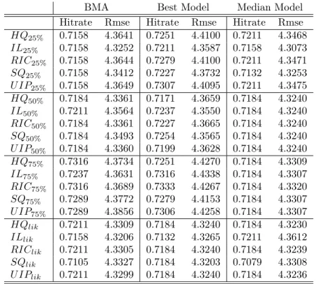
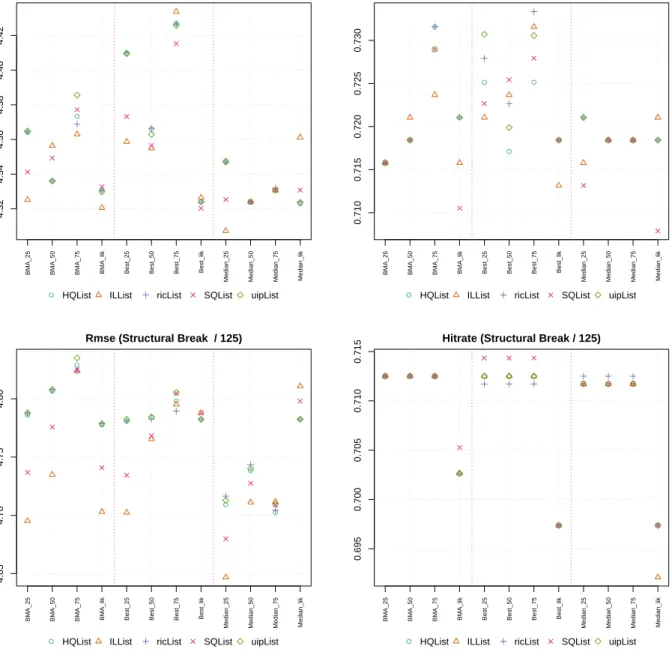
Table 3 and Figure 1 summarize results for setup A. The top panel of Figure 1 illustrates the forecasting accuracy in terms of the rmse statistic. The picture reveals that the highest posterior probability model (best model) shows largest variation with respect to the choice of the g-prior and the size of the hold-out sample. On the other end of the rmse statistic is the median model: here the rmse is minimized for theILprior with a hold-out size of 25% of the total sample. Note also that the variation for the median model is relatively small except the forecasts based on the marginal likelihood (medlik). Model averaged forecasts fall somewhat between the best model forecasts and the ones of the median model. In general the ranking of prior structures is quite stable across both hold-out sample sizes and forecast approaches with the IL prior dominating the other priors for g. Results differ when looking at the direction of change statistic. Here the median model always underperforms model averaged and best model forecasts. Also the prior choice for g seems to be of minor importance in comparison to the choice of the hold-out sample. The best results are obtained retaining 75% of the available observations, a recommendation made by Eklund and Karlsson (2007). Under setting ’B’ a structural break (or regime switch) occurs at the middle of the sample period (observation 125). Results are summarized in Table 4 and Figure 1. Turning first to forecast accuracy the bottom panel of picture 1 shows that again the median model does best in minimizing the rmse statistic. However, this time there is considerably more variation of the rmse. Likelihood averaged forecasts, especially, are performing by far worse as the ones based on the predictive likelihood. This result is not surprising since one merit of the predictive likelihood is its ’robustness’ against the occurrence of structural breaks (Eklund and Karlsson (2007)). Results for the best model are more concentrated with the rmse lying above the median model. On average, averaged forecasts do better than the ones based on the highest posterior model but again worse than the median model forecasts. Regarding the prior structures forg, as in the previous setting ’A’, theILprior yields the best forecasts followed by theSQprior. Concerning direction of changes all priors and forecast approaches perform very similarly with only the likelihood based forecasts falling well off the others. Concluding the simulation results indicate that forecast accuracy measured by the rmse is highest for the median probability model dominating both, averaged and best model forecasts. Direction of changes are better captured by averaged forecasts where the hold-out sample size should be around 75% of the total sample. On the other hand, the rmse
statistic is minimized retaining 25% of the total available observations. Concerning the prior structures for g, the IL prior dominates the other settings, followed by the SQ prior. This suggests that the benchmark prior put forward by Fernández et al. (2001a) is not optimal in a predictive sense when the underlying likelihood is the predictive instead of the marginal.
3
Empirical Application: Forecasting Industrial
Produc-tion
Bayesian model averaging is applied to data on industrial output for six CESEE economies: the Czech Republic, Hungary, Poland, and Bulgaria, Romania and Slovenia. These countries represent the largest economies in terms of economic activity and population in the region. For the six countries the series is published with a time lag of 1-2 months. Consequently we focus on the 1 step ahead forecasting horizon in order to compensate for the publication lag. Note that we use univariate (country specific) models as opposed to modeling industrial production in a country-wide system - for example by means of vector autoregressive models (VAR). Marcellino et al. (2003) compare several forecasting models for euro area forecasts of the industrial production index and conclude that (aggregated) univariate forecasts perform better than in a multivariate setting. Also, a short forecast horizon - as is the case in this application - plays in favor of univariate models. The data we use comprises up to 15 potential explanatory variables and is described in more detail in the appendix (see also Table 2).
As outlined in Section 1.1 we choose a linear forecasting model following Marchetti and Parigi (2000) and Zizza (2002). In particular the forecasting model for country i is of the form: yt =α+ 2 X j=1 X(t−j)β+I(i) 3 X k=1 energy(t−k)γ+seasonalsθ+ut (7)
with α denoting a constant and u the iid error term. By seasonals we denote monthly
dummy variables in order to account for the cyclical pattern of the data. The variable
energy denotes energy consumption and is separated from the remaining variables that are captured by the design matrix X. The reason for this is the varying degree of timeliness with respect to availability of the time series. For most of the countries publication of the energy series occurs with a lag of two months. Only for Hungary the data is right available with the industrial production index itself. The indicator function I(i) is therefore country specific governing the order of lags of the energy variable. All remaining variables are lagged for one and two time periods (including the dependent variable that is contained in X). Out-of-sample statistics are calculated over a 30-period horizon and are based on rolling regressions with an enlarging estimation window. Based on the simulation study carried out in Section 2.1 we elicit theILprior forg.7 We decide to choose a hold-out sample size of 50%
that lies in between the 25% and 75% recommendations. Since the first rolling regressions are based on 60 (Czech Republic, Hungary and Poland) and 70 (Bulgaria, Romania and Slovenia) observations, 50% of the data seems to be the maximum one can retain for model comparison.
7The model size prior is the same as in the simulation study, that is binomial-beta anchored on a prior
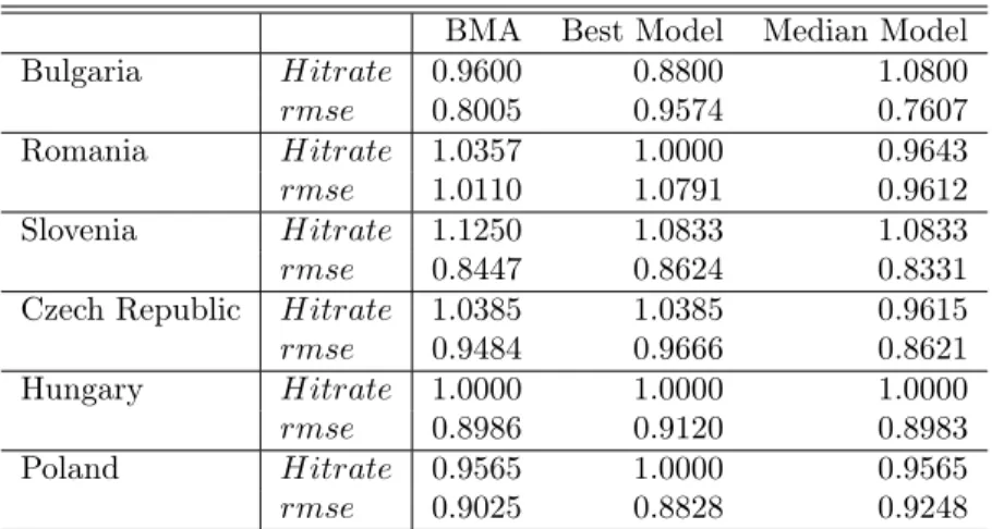
The results are summarized in Table 4, in the appendix where we have normalized the statistics relative to an AR (1) benchmark model. Consequently values above 1 for the hitrate statistic and values below 1 for the rmse indicate that the benchmark model is outperformed by the respective forecasting alternative. Note that we have included the seasonal dummy variables in the AR (1) baseline model as additional exogenous regressors in order to allow for a fair comparison.
Model averaging excels in forecasting the industrial production in terms of direction of changes: the hitrate ranges from 80% to 96% pointing to an extraordinarily high degree of correctly forecast directions of the underlying time series. This suggest that the sideward movements in the data can almost exclusively be traced back to the cyclical patterns and consequently be properly modeled by inclusion of the seasonal dummy variables. The AR (1) benchmark model can only beat model averaged forecasts for the cases of Bulgaria and Poland. Note that there is in general a great deal of variation regarding which and how many variables serve as good predictors.8 While in the Czech Republic and Hungary the median model is typically very saturated with the mean number of regressors around 20 (not including the seasonals), in Poland and Bulgaria the posterior mass is very concentrated on 2-3 regressors only. Regarding the precision of the forecasts, the median model turns out to be the forecast approach that minimizes the forecasting error as measured by the rmse. With the exception of Poland this finding holds true for all countries covered in the data set. Furthermore, the median model clearly outperforms the AR (1) benchmark model for all six countries. Hence, although the size of the median model varies strongly across the countries with some sharing on average a very large number of explanatory variables, it still dominates the other approaches in terms of forecast accuracy.
4
Conclusions
In this paper we investigated the predictive performance of various forecasting approaches. We first compared forecasts based on the marginal likelihood traditionally employed in BMA to that based on the predictive likelihood - a measure that accounts for the model’s forecast quality. We further looked at three alternative ways how to compute forecasts. Based on a simulation study our results imply that direction of changes are best forecast using averaged forecasts, a result that is in line with Crespo Cuaresma (2007). On the other hand, forecast accuracy as measured by the root mean square error is largest under the so-called median model proposed by Barbieri and Berger (2003). With respect to prior choice our results show that the best forecast results are obtained when drawing on the ILprior (Laud and Ibrahim (1995)), a prior that implies a considerably smaller value for g than under the prominent ’benchmark prior’ put forward by Fernández et al. (2001a). In particular best results in terms of forecast accuracy are obtained under the IL prior with a hold-out sample size of
25%of the total data, whereas averaged forecasts excel in forecasting the direction of changes with a considerably larger hold-out size of 75% of the data. In the empirical application we
8A common finding is that for all countries the lagged dependent variable (industOut
1) appears among the
most important regressors. Moreover, energy consumption carries valuable information about the industrial production throughout all countries. This finding appears robust in the data despite the fact that in most countries the variable is included with a time lag of order 3 due to the availability problems of the time series. In an experiment not reported in this paper including first lags of the energy variable for all countries, the variable appeared as the most important predictor for the industrial production index.
forecast the industrial production index for six CESEE countries with a forecast horizon of 1 step ahead. The analysis shows that the industrial production index based on the proposed forecast strategies and prior choices can be forecast to a satisfactory degree outperforming the simple AR (1) benchmark model in most of the cases. Finally, model averaging reveals a range of important variables serving as good leading indicators. Among them industrial and economic sentiment indicators as well as energy consumption carry valuable information about the future development of industrial output.
References
Avramov, D. (2002). Stock Return Predictability and Model Uncertainty. Journal of Finan-cial Economics, 64:423–458.
Barbieri, M. M. and Berger, J. O. (2003). Optimal Predictive Model Selection. Ann. Statist., 32:870–897.
Bates, J. and Granger, C. (1969). The Combination of Forecasts. Operations Research
Quarterly, 20:451–468.
Bodo, G., Golinelli, R., and Parigi, G. (2000). Forecasting industrial production in the Euro area. Empirical Economics, 25:541–561.
Cremers, M. K. (2002). Stock Return Predictability: A Bayesian Model Selection Perspec-tive. The Review of Financial Studies, 15(4):1223–1249.
Crespo Cuaresma, J. (2007). Forecasting euro exchange rates: How much does model aver-aging help? University of Innsbruck, mimeo.
Eklund, J. and Karlsson, S. (2007). Forecast Combination and Model Averaging using
Predictive Measures. Econometric Reviews, 26:329–362.
Feldkircher, M. and Zeugner, S. (2009). Benchmark Priors Revisited: On Adaptive
Shrink-age and the Supermodel Effect in Bayesian Model Averaging. IMF Working Paper,
WP/09/202.
Fernández, C., Ley, E., and Steel, M. F. (2001a). Benchmark Priors for Bayesian Model Averaging. Journal of Econometrics, 100:381–427.
Fernández, C., Ley, E., and Steel, M. F. (2001b). Model Uncertainty in Cross-Country Growth Regressions. Journal of Applied Econometrics, 16:563–576.
Foster, D. P. and George, E. I. (1994). The Risk Inflation Criterion for Multiple Regression.
The Annals of Statistics, 22:1947–1975.
Geweke, J. and Whiteman, C. (2006). Handbook of Economic Forecasting, volume 1, chapter Bayesian Forecasting, pages 3–80. Elsevier.
Hamilton, J. D. (2008).The New Palgrave Dictionary of Economics. Second Edition, chapter Regime Switching Models. Palgrave Macmillan.
Kapetanios, G., Labhard, V., and Price, S. (2008). Forecasting using Bayesian and infor-mation theoretic model averaging: an application to UK inflation. Journal of Business Economics and Statistics, 26:33–41.
Kapetanios, G., Vincent, L., and Price, S. (2006). Forecasting Using Predictive Likelihood Model Averaging. Economics Letters.
Kass, R. and Wasserman, L. (1995). A reference Bayesian test for nested hypotheses and its relationship to the Schwarz criterion. Journal of the American Statistical Association, pages 928–934.
Koop, G. (2003). Bayesian Econometrics. John Wiley & Sons.
Laud, P. and Ibrahim, J. (1995). Predictive model selection. Journal of the Royal Statistical Society, Series B 57:247–262.
Laud, P. and Ibrahim, J. (1996). Predictive specification of prior model probabilities in variable selection. Biometrika, 83:267–274.
Ley, E. and Steel, M. F. (2009). On the Effect of Prior Assumptions in Bayesian Model Averaging with Applications to Growth Regressions. Journal of Applied Econometrics, 24:4:651–674.
Liang, F., Paulo, R., Molina, G., Clyde, M. A., and Berger, J. O. (2008). Mixtures of g Priors for Bayesian Variable Selection. Journal of the American Statistical Association, 103:410–423.
Madigan, D. and York, J. (1995). Bayesian graphical models for discrete data. International Statistical Review, 63.:215–232.
Marcellino, M., Stock, J., and Watson, M. (2003). Macroeconomic forecasting in the euro area: country specific versus area-wide information. European Economic Review, 47:1–18. Marchetti, D. J. and Parigi, G. (2000). Energy Consumption, Survey Data and the Predic-tion of Industrial producPredic-tion in Italy: a comparison and combinaPredic-tion of different models.
Journal of Forecasting, 19:419–440.
Raftery, A. E. (1995). Bayesian Model Selection in Social Research.Sociological Methodology, 25:111–163.
Sala-i-Martin, X., Doppelhofer, G., and Miller, R. I. (2004). Determinants of Long-Term
Growth: A Bayesian Averaging of Classical Estimates (BACE) Approach. American
Eco-nomic Review, 94:813–835.
Wright, J. (2003). Bayesian Model Averaging and Exchange Rate Forecasts. Board of
Governors of the Federal Reserve System, International Discussion Paper, Nr. 779. Zizza, R. (2002). Forecasting the industrial production index for the euro area through
Appendix
MCMC samplerThis section briefly discusses the MCMC sampler used throughout the paper. Exploring the model space can be done via a range of search algorithms, here Markov Chain Monte Carlo methods are used, which have been shown to have good properties in the framework of BMA. The Markov chain is designed to wander efficiently through the model space, where it draws attention solely to models with non-negligible posterior mass.
The sampler uses a birth/deathM C3 (Madigan and York, 1995) search algorithm to explore
the model space. In each iteration step a candidate regressor is drawn from kc ∼ U(1, K). A (birth step) is adding the candidate regressor to the current model Mj if that model did not already includekc. On the other hand, the candidate regressor is dropped if it is already contained in Mj (death step). This is in the vein of Madigan and York (1995) with the new model always being drawn from a neighborhood of the current one differing only by a single regressor. To compare the sampled candidate model Mi to the current one, the posterior odds ratio is calculated implying the following acceptance probability,
˜ pij = min 1, p(Mi)p(Y|Mi) p(Mj)p(Y|Mj) . (8)
Model Space Prior
A typical way of prior specification is to discriminate among models according to the number of regressors they include. Assuming that each covariate enters the regression with proba-bility ϑ the prior mass for model j amounts to p(Mj) =ϑkj(1−ϑ)K−kj. In most empirical studiesϑ is now fixed to1/2which results into equal model probabilities of2−K for all mod-els. Consequently the posterior odds ratio resembles solely the Bayes factor and comparison of models is governed by their relative likelihoods. However, this prior structure is not as non-informative as it sounds at first sight. Ley and Steel (2009) show that fixing ϑ = 1/2
puts most mass on models with K/2 regressors since they are dominant in number. Their recommendation is thus to treat ϑ as random and placing a prior on it. In particular the expected model size follows a binomial-beta distribution:
P(k=kj) = Γ(1 +b) Γ(1) + Γ(b) + Γ(1 +b+K) K kj Γ(1 +kj)Γ(b+K−kj) kj = 0, . . . , K (9)
The parameter to be elicited isµthe prior expected model size.9 By applying the
binomial-beta hyperprior we considerably deviate from previous studies that have employed BMA for forecasting purposes. Ley and Steel (2009) demonstrate the risk and the influence a poorly specified prior exerts on posterior results when ϑ is fixed. The relative merits of BMA tend to be less pronounced and its predictive power deteriorates. In contrast, with the hyperprior the choice of µhas no influential impact on posterior inference and the prior over models is purely non-informative.
Data Description
The data we use is briefly described in Table 2 and is available on a monthly basis from Eurostat. It comprises the time span from January 2001 to September 2009 for Bulgaria, Slovenia and Romania. For the Czech Republic, Hungary and Poland the data period is about one year shorter (January 2002 to September 2009). As explanatory variables poten-tially leading the industrial production series we choose the construction output, industrial sales, the unemployment rate, retail trade, manufacturing orders and various sentiment in-dicators. These sentiment indicators are conducted via surveys and quantified in balances of positive and negative replies. Note that there exist several ways of transforming these raw series by either taking lags or spreads of the data. This further enlarges the model space thereby raising the potential for (model) uncertainty. All variables have been tested for a unit root by the augmented Dickey Fuller test.10 After linearly detrending the data
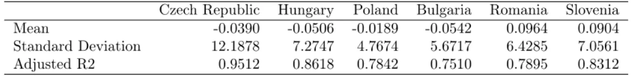
all variables in question - including the dependent one - pass the test for stationarity. The highly cyclical nature of the data was already noted in Bodo et al. (2000) who analyzed the monthly industrial production index for the euro area. In particular, in Table 1 the vari-ation explained by seasonal dummy variables and a constant ranges from 75% (Bulgaria) to 95% (Czech Republic). Note also the difference in the summary statistics: the index is most volatile in the Czech Republic, whereas the other countries show a similar degree of variation.
Czech Republic Hungary Poland Bulgaria Romania Slovenia
Mean -0.0390 -0.0506 -0.0189 -0.0542 0.0964 0.0904
Standard Deviation 12.1878 7.2747 4.7674 5.6717 6.4285 7.0561
Adjusted R2 0.9512 0.8618 0.7842 0.7510 0.7895 0.8312
Table 1: Summary Statistics of the detrended industrial production index over the whole sample period. The adjusted R2 refers to the variation of the data explained by only seasonal components and an intercept term.
Tables and Figures
10The test specification included a constant and a trend. Results are available from the author upon
V ariable Abbreviation Description Industrial Pro duction (industOut) constan t prices, w orking da y adjusted, Index, 199 8 = 100 Construction Output (constOut) cons ta n t prices, w orking da y adjusted, Index 1998=100 Industrial Sales (industSales) curren t prices, unadjusted , Index, 1998 = 1 00 Unemplo ymen t rate (unempl) LFS metho dology , seasonally adjusted Retail trade (retailT rade) constan t prices, w ork in g da y adjusted Index, 1998 = 100 Gross Energy Consumption (energy) ele ctrical energy in giga w att hours Man ufacturing orders ( indust or der s ) curren t prices, unadjusted, Index, 2005 = 100 Man ufacturing exp ort or d ers ( industO r der sexp ) curren t prices , unadjusted, Index, 20 05 = 100 Qualitativ e Data: Sen timen t Indic a tors are deriv ed from surv eys rep orting the balance b e tw een the p erc en tage of p ositiv e and negativ e replies. Economic sen timen t indicator (ecoSen t) seasonally adjusted, balance Industrial sen timen t indicator (industSen t) seasonally adjusted, balance Industrial sen timen t indicator for EU ( industS ent eu ) seasonally adjusted, balance Construction confide nce indicator (ConstructionSen t) seasonally adjusted, balance Retail confidence indicator (RetailSen t) seasonally adjusted, balance Consumer confide nce indicator (ConsumerSen t) seasonally adjusted, balance Assessmen t of exp ort order-b o ok lev els (expOrders) seasonally adjusted, balance T able 2: Data description. Industrial pro duction refers to output of the Mining and quar rying, m a n ufacturing, electricit y , gas, steam and air conditioning supply industries; industrial sales to that of mining, q u a rrying and man ufacturing. Retail trade e x c ludes that of motor v eh icles and motorcycles. All data are from Euros tat.
BMA Best Model Median Model Hitrate Rmse Hitrate Rmse Hitrate Rmse HQ25% 0.7158 4.3641 0.7251 4.4100 0.7211 4.3468 IL25% 0.7158 4.3252 0.7211 4.3587 0.7158 4.3073 RIC25% 0.7158 4.3644 0.7279 4.4100 0.7211 4.3471 SQ25% 0.7158 4.3412 0.7227 4.3732 0.7132 4.3253 U IP25% 0.7158 4.3649 0.7307 4.4095 0.7211 4.3475 HQ50% 0.7184 4.3361 0.7171 4.3659 0.7184 4.3240 IL50% 0.7211 4.3564 0.7237 4.3550 0.7184 4.3240 RIC50% 0.7184 4.3361 0.7227 4.3665 0.7184 4.3240 SQ50% 0.7184 4.3493 0.7254 4.3565 0.7184 4.3240 U IP50% 0.7184 4.3360 0.7199 4.3628 0.7184 4.3240 HQ75% 0.7316 4.3734 0.7251 4.4270 0.7184 4.3309 IL75% 0.7237 4.3631 0.7316 4.4338 0.7184 4.3307 RIC75% 0.7316 4.3689 0.7333 4.4267 0.7184 4.3320 SQ75% 0.7289 4.3772 0.7279 4.4153 0.7184 4.3307 U IP75% 0.7289 4.3856 0.7306 4.4258 0.7184 4.3307 HQlik 0.7211 4.3309 0.7184 4.3240 0.7184 4.3230 ILlik 0.7158 4.3206 0.7132 4.3265 0.7211 4.3612 RIClik 0.7211 4.3305 0.7184 4.3240 0.7184 4.3239 SQlik 0.7105 4.3327 0.7184 4.3203 0.7079 4.3308 U IPlik 0.7211 4.3299 0.7184 4.3240 0.7184 4.3236
Table 3: M-Open Setting. Top panel is based on a hold-out sample of 25%, second panel on 50%, third panel on 75% and bottom panel on likelihood averaging.
BMA Best Model Median Model
Hitrate Rmse Hitrate Rmse Hitrate Rmse HQ25% 0.7125 4.7861 0.7125 4.7808 0.7117 4.7092 IL25% 0.7125 4.6953 0.7125 4.7024 0.7117 4.6469 RIC25% 0.7125 4.7879 0.7117 4.7810 0.7125 4.7164 SQ25% 0.7125 4.7368 0.7143 4.7344 0.7117 4.6798 U IP25% 0.7125 4.7877 0.7125 4.7823 0.7117 4.7130 HQ50% 0.7125 4.8066 0.7125 4.7839 0.7117 4.7381 IL50% 0.7125 4.7349 0.7125 4.7655 0.7117 4.7111 RIC50% 0.7125 4.8080 0.7117 4.7825 0.7125 4.7434 SQ50% 0.7125 4.7757 0.7143 4.7683 0.7117 4.7275 U IP50% 0.7125 4.8078 0.7125 4.7843 0.7117 4.7402 HQ75% 0.7125 4.8289 0.7125 4.7980 0.7117 4.7024 IL75% 0.7125 4.8237 0.7125 4.7951 0.7117 4.7117 RIC75% 0.7125 4.8239 0.7117 4.7894 0.7125 4.7043 SQ75% 0.7125 4.8249 0.7143 4.8046 0.7117 4.7088 U IP75% 0.7125 4.8349 0.7125 4.8054 0.7117 4.7097 HQlik 0.7026 4.7776 0.6974 4.7824 0.6974 4.7824 ILlik 0.7026 4.7031 0.6974 4.7879 0.6921 4.8107 RIClik 0.7026 4.7787 0.6974 4.7824 0.6974 4.7824 SQlik 0.7053 4.7410 0.6974 4.7878 0.6974 4.7979 U IPlik 0.7026 4.7786 0.6974 4.7824 0.6974 4.7824
Table 4: Structural Break Setting (125). Top panel is based on a hold-out sample of 25%, second panel on 50%, third panel on 75% and bottom panel on likelihood averaging.
● ● ● ● ● ● ● ● ● ● ● ● 4.32 4.34 4.36 4.38 4.40 4.42 Rmse (M−open)
BMA_25 BMA_50 BMA_75 BMA_lik Best_25 Best_50 Best_75 Best_lik
Median_25 Median_50 Median_75 Median_lik
● HQList ILList ricList SQList uipList
● ● ● ● ● ● ● ● ● ● ● ● 0.710 0.715 0.720 0.725 0.730 Hitrate (M−open)
BMA_25 BMA_50 BMA_75 BMA_lik Best_25 Best_50 Best_75 Best_lik
Median_25 Median_50 Median_75 Median_lik
● HQList ILList ricList SQList uipList
● ● ● ● ● ● ● ● ● ● ● ● 4.65 4.70 4.75 4.80
Rmse (Structural Break / 125)
BMA_25 BMA_50 BMA_75 BMA_lik Best_25 Best_50 Best_75 Best_lik
Median_25 Median_50 Median_75 Median_lik
● HQList ILList ricList SQList uipList
● ● ● ● ● ● ● ● ● ● ● ● 0.695 0.700 0.705 0.710 0.715
Hitrate (Structural Break / 125)
BMA_25 BMA_50 BMA_75 BMA_lik Best_25 Best_50 Best_75 Best_lik
Median_25 Median_50 Median_75 Median_lik
● HQList ILList ricList SQList uipList
Figure 1: Forecast performance calculated over 20 out-of-sample forecasts averaged over 30 Monte Carlo steps. Top panel belongs to setting ’A’ whereas bottom panel is based on setting ’B’.
BMA Best Model Median Model Bulgaria Hitrate 0.9600 0.8800 1.0800 rmse 0.8005 0.9574 0.7607 Romania Hitrate 1.0357 1.0000 0.9643 rmse 1.0110 1.0791 0.9612 Slovenia Hitrate 1.1250 1.0833 1.0833 rmse 0.8447 0.8624 0.8331
Czech Republic Hitrate 1.0385 1.0385 0.9615
rmse 0.9484 0.9666 0.8621
Hungary Hitrate 1.0000 1.0000 1.0000
rmse 0.8986 0.9120 0.8983
Poland Hitrate 0.9565 1.0000 0.9565
rmse 0.9025 0.8828 0.9248
Table 5: Forecast results compared to AR (1) benchmark model. Values above (below) 1 for the hitrate (rmse) indicate better predictive performance than the benchmark model.