Hi-Stat
Discussion Paper Series
No.178
Subsampling-Based Tests of Stock-Return Predictability In Choi
Timothy K. Chue July 2006
Hitotsubashi University Research Unit for Statistical Analysis in Social Sciences
A 21st-Century COE Program
Institute of Economic Research Hitotsubashi University Kunitachi, Tokyo, 186-8603 Japan
Subsampling-Based Tests of Stock-Return Predictability
In Choiyand Timothy K. Chuez
First Draft: March 2006 This Draft: June 2006
Abstract
We develop subsampling-based tests of stock-return predictability and ap-ply them to U.S. data. These tests allow for multiple predictor variables with local-to-unit roots. By contrast, previous methods that model the predictor vari-ables as nearly integrated are only applicable to univariate predictive regressions. Simulation results demonstrate that our subsampling-based tests have desirable size and power properties. Using stock-market valuation ratios and the risk-free rate as predictors, our univariate tests show that the evidence of predictability is more concentrated in the 1926–1994 subperiod. In bivariate tests, we …nd sup-port for predictability in the full sample period 1926–2004 and the 1952–2004 subperiod as well. For the subperiod 1952–2004, we also consider a number of consumption-based variables as predictors for stock returns and …nd that they tend to perform better than the dividend–price ratio. Among the variables we consider, the predictive power of the consumption–wealth ratio proposed by Let-tau and Ludvigson (2001a, 2001b) seems to be the most robust. Among variables based on habit persistence, Campbell and Cochrane’s (1999) nonlinear speci…-cation tends to outperform a more traditional, linear speci…speci…-cation.
Keywords: Subsampling, local-to-unit roots, predictive regression, stock-return predictability, consumption-based models.
1
Introduction
The …nance profession has a long-standing interest in the study of stock-market pre-dictability. For practitioners, having the ability to forecast future stock returns is clearly valuable for asset-allocation decisions. For academics, whether or not stock
This paper was presented at the Hitotsubashi University. We thank the seminar participants, es-pecially Taku Yamamoto, for helpful comments. The …rst author acknowledges …nancial support from the RGC Competitive Earmarked Research Grant 2003–2004 under Project No. HKUST6223/03H.
yDepartment of Economics, Hong Kong University of Science and Technology, Clear Water Bay,
Kowloon, Hong Kong. E-mail: [email protected]. Home page: http://ihome.ust.hk/~inchoi.
zDepartment of Economics, Hong Kong University of Science and Technology, Clear Water Bay,
returns are predictable and by which variables they can be predicted a¤ect how the stock market should be modelled theoretically. For example, the theories proposed by Campbell and Cochrane (1999), Lettau and Ludvigson (2001a, 2001b), Lustig and Van Nieuwerburgh (2005), Piazzesi, Schneider, and Tuzel (2006), Santos and Veronesi (2006), and Yogo (2006) all have testable implications regarding stock-return predictability.
Early studies of predictability rely on standard asymptotic distribution theory to draw inference. Examples of such studies include the works by Fama and Schwert (1977), Keim and Stambaugh (1986), Campbell (1987), Campbell and Shiller (1988), Fama and French (1988, 1989), and Hodrick (1992). However, as more recent studies have pointed out (see Elliott and Stock, 1994, and Stambaugh, 1999, for example), standard asymptotic distribution theory works poorly when the predictor variable is persistent and its innovations are highly correlated with stock returns.
To evaluate the evidence of predictability in this setting, new tests that model the predictor variable as nearly integrated have been developed. In particular, Torous, Valkanov, and Yan (2004) and Campbell and Yogo (2005) both use Bonferroni meth-ods to derive tests that allow the predictor variable to contain a local-to-unit root.1 Although these tests perform much better than the conventionalt-tests, it is not clear how the Bonferroni methods can be extended to a multiple-predictive regression.
In practice, however, the need to carry out tests for multiple-predictive regressions is pressing because the theoretical models mentioned in the …rst paragraph suggest di¤erent variables that could be used to forecast returns. To examine the marginal and/or joint predictive power of these variables, we need to conduct statistical tests in a multivariate setting. Since many of these variables are highly persistent, using standard asymptotics for inference can be misleading. In the current literature, there is not yet any procedure that can test for predictability in the presence of multiple, nearly integrated regressors.
In this paper, we …ll this void by developing subsampling-based predictability tests of that allow for multiple regressors with local-to-unit roots. The subsampling approach computes the statistic of interest for subsamples of the data (consecutive sample points in the case of time-series data) and the statistic’s subsampled values are used to estimate its …nite-sample distribution.2 Romano and Wolf (2001) and Choi (2005b) examine the performance of subsampling when it is used to analyze time series with exact unit roots. In this study, we prove the validity of subsampling for time series with local-to-unit roots.
Since subsampling does not require the estimation of nuisance parameters, apply-ing the procedure to a multiple-regression settapply-ing is no more di¢ cult than applyapply-ing it to a simple regression. By contrast, previous tests proposed by Torous et al. (2004) and Campbell and Yogo (2005) require the estimation of the degree of persistence of the predictor variables. These studies use Bonferroni methods to carry out this
1
Valkanov (2003) also uses the local-to-unit root setup to examine stock-return predictability. Valkanov’s methodology relies on a long-run restriction between the dividend–price ratio and stock returns implied by the dynamic Gordon growth model. This methodology is not applicable to predictor variables that do not have such a long-run relationship with stock returns.
estimation in univariate tests, but multivariate extensions of their approaches seem infeasible. Wolf (2000) also uses subsampling methods to study predictive regres-sions, but he only examines a model with a single stationary regressor. Lanne (2002) makes use of stationarity tests to carry out inference on stock-return predictability. He allows the predictor variables to be nearly integrated, but bases his inference on stock-return data alone and ignores data on the predictor variables altogether. As Campbell and Yogo (2005) argue, such an approach tends to have poor power when the predictor variable is persistent but remains su¢ ciently far from being integrated. Finally, the bootstrap may seem to be a feasible alternative to subsampling, but it can be shown to be inconsistent for regressions with nearly integrated regressors. Basawa et al. (1991), Datta (1996), and Choi (2005a) demonstrate the failure of the bootstrap for the AR(1) and VAR models. One major strength of subsampling is that it can work even when the bootstrap method fails.
Our subsampling-based tests suggest that the evidence for stock-return predictabil-ity using stoc-market valuation ratios and the risk-free rate is quite strong. Our univariate tests show that the evidence is more concentrated in the subperiod from 1926–1994. In bivariate tests, we …nd evidence for predictability in the full sample period, 1926–2004, and the subperiods 1926–1994 and 1952–2004. We also demon-strate the value of being able to carry out joint tests— there are numerous cases where univariate tests are insigni…cant, but joint tests are not negligible.
We also show that a number of consumption-based variables have predictive power for stock returns in the subperiod 1952–2004. During this period, these variables tend to be better predictors for stock returns than the dividend–price ratio. Among the variables we consider, the predictive power of the consumption–wealth ratio (cay) proposed by Lettau and Ludvigson (2001a, 2001b) seems to be the most robust. Among variables that are based on habit persistence, Campbell and Cochrane’s (1999) nonlinear speci…cation tends to outperform a more traditional linear speci…cation.
The rest of the paper is organized as follows. Section 2 introduces the model and test statistics for predictive regressions. Section 3 proposes subsampling-based meth-ods for predictive regressions with one regressor. Section 4 extends the subsampling method of Section 3 to multiple regressions. Section 5 reports simulation results. Section 6 presents our empirical …ndings on stock-market predictability. Section 7 concludes. We relegate technical results to the appendices.
2
The model and test statistics for predictive regressions
Consider the simple linear regression model
yt= + xt 1+uyt; (t= 2; : : : ; T); (1)
where
xt = +vt; (2)
vt = vt 1+uvt; = ec=T; c2R:
Model (1) is the prototypical predictive regression model that has been widely used in the …nance literature. For instance, yt denotes the excess stock return in period t
and xt 1 is a variable observed at time period t 1 that may be able to predict yt.
In order to predict the excess stock return, such variables as interest rates, default spreads, dividend yield, the book-to-market and earnings–price ratios have been used. Modellingxt as a nearly integrated process3 as in (2) re‡ects the fact that many
predictors used in the …nance literature are quite persistent. Campbell and Yogo (2005) report that the respective 95% con…dence intervals for are [0.957, 1.007] and [0.939,1.000] for the dividend–price and earnings–price ratios they studied. The mod-elling has also been used in the …nance literature including Valkanov (2003), Torous et al. (2004), and Campbell and Yogo (2005). These articles use the representation = 1 +c=T, but this is equivalent to our speci…cation (2) for asymptotic analysis. We prefer using representation (2) because it simpli…es the proofs in Appendixes I and II.
In model (1), it is reasonable to assume thatuytanduvt are correlated. For exam-ple, ifxtandytdenote the dividend yield and the excess stock return, respectively, an
increase in stock price will decrease the dividend yield and increase the stock return. More speci…cally, we assume
Assumption 1 Let kakp= (Ejajp)1=p. Suppose
(i) uyt= uvt+et whereuvs is independent of et for everysand t.
(ii) ut = fuvt; etg is strictly stationary with E(u1) = 0 and Eku1k2+ < 1 for >0;
(iii) futgis strong mixing with its mixing coe¢ cients u;msatisfying, for >0,
1
X m=1
=(2+ )
u;m <1:
Assumption 1 allows serial correlations in fuytg and fuvtg and cross-sectional correlations between uyt and uvs. Most previous studies have assumed white noise
processes forfuvtgandfuytg. Assumption 1 generalizes this, though in most …nancial
applications it su¢ ces to assume fuvtg andfuytg are uncorrelated. In addition, it is not necessary to model the form of the serial correlation in futg in this study. Under
Assumption 1, the functional central-limit theorem for futg also holds (cf. Phillips
and Durlauf, 1986).
The null hypothesis we are interested in is
H0 : = 0: (3)
In most cases, we will set 0 = 0, which corresponds to the unpredictability of yt.
3
For null hypothesis (3), we may consider the usualt-test:
t( 0) = r ^ 0
^2y PTt=2(xt 1 x 1)2
1; (4)
where ^ is the OLS estimator of , x 1 = T11PTt=2xt 1, and ^2y is the usual
esti-mator of 2y =E(u2yt). The asymptotic distribution oft( 0) for the case of serially uncorrelated fuytgis given (cf. Elliott and Stock, 1994) in the relation
t( 0)) R1 0 Jc(r)dW(r) qR1 0 Jc(r)2dr +p1 2Z; asT ! 1; where)denotes weak convergence,Jc(r) =Jc(r)
R1
0 Jc(s)ds; Jc(r)is an Ornstein– Uhlenbeck process generated by the stochastic di¤erential equationdJc(r) =cJc(r)dr+ dW(r) with the initial condition Jc(0) = 0 and the standard Brownian motion W(r); =Corr(uyt; uvt), andZ =d N(0;1), is independent of (W(r); Jc(r)). Unless = 0, the distribution of the t-test depends on the nuisance parameters c and , which makes it di¢ cult to use it for statistical inference.
Under Assumption 1, model (1) can be rewritten as
yt= 0+ xt 1+ (xt xt 1) +et; (5)
where 0 = (1 ) . Note that the regressors are totally exogenous in model (5) such that the OLS estimator of has a mixture normal distribution in the limit. Lettingxt 1 be the residual obtained by regressingxt 1 onf1; xt xt 1g, thet-test for null hypothesis (3) is de…ned by
Q( 0; ) = r ~ 0 ^2e PTt=2x 2
t 1
1; (6)
where ~ is the OLS estimator of using model (5) and ^2e is the usual estimator of 2
e =E(e2t). TheQ( 0; )test is designed for serially uncorrelatedfetgand has some
optimal properties as discussed in Campbell and Yogo (2005). If fetg are serially
correlated, ^2e should be replaced with the long-run variance estimator (see, e.g., Andrews, 1991). The Q( 0; ) weakly converges to a standard normal distribution.
In practice, however, the Q( 0; ) test is not feasible since the value of is un-known. If we choose = 1, it is asymptotically equivalent to Lewellen’s (2004) bias-adjusted test, though the functional forms of Q( 0;1) and Lewellen’s test are di¤erent. When = 1, Q( 0;1))Z r c 2 e 2v R1 0 Jc(r)2dr 1; asT ! 1: (7)
Again, the limiting distribution given in (7) involves nuisance parameters in a compli-cated way. Iffetgis serially correlated as in Assumption 1, the limiting distribution
3
Subsampling test statistics
3.1 Subsampling
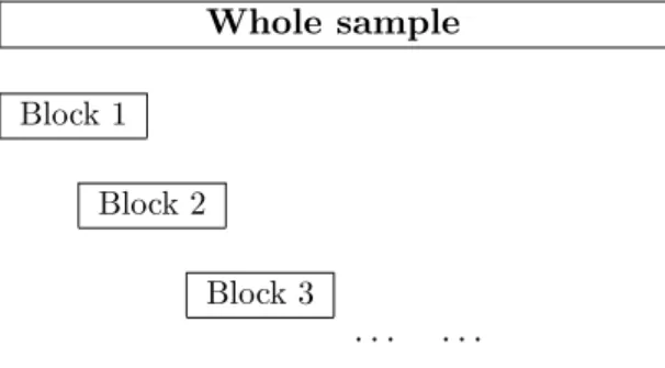
It was shown in Section 2 thatt( 0)andQ( 0;1)have limiting distributions that de-pend on inestimable parameters. Conventional asymptotic methods cannot be used for this reason. To remedy the situation, this section proposes using subsampling as a way to …nd approximations to the limiting distributions of the test statistics t( 0) andQ( 0;1). Using smaller blocks of consecutively observed time series, the subsam-pling method computest( 0)andQ( 0;1), and then formulates empirical cumulative distribution functions using the computed values of the statistics. Subsample critical values are obtained from the empirical distribution functions. We use consecutively observed time series to retain the serial correlation structure present in the data. In addition, blocks may share common sample points. Figure 1 illustrates the scheme of formulating blocks for the subsampling method. The method explained so far is called uncentered subsampling, the meaning of which will become obvious shortly.
Whole sample Block 1
Block 2 Block 3
Figure 1: Blocks for Subsampling Method
To be more speci…c, let tb;s( 0) be the t-test that uses the subsample f(ys; xs), : : :,(ys+b 1; xs+b 1)g. We de…ne Qb;s( 0;1)in the same way. The number of sample points in the subsample is b, which is called the block size. Index s denotes the starting point of the subsample. In this subsampling scheme, there will be T b+ 1 blocks with size b. Now, consider the empirical distribution functions using tb;s( 0) and Qb;s( 0;1) LtT(x) = 1 T b+ 1 TXb+1 s=1 1ftb;s( 0) xg; (8) LQT(x) = 1 T b+ 1 TXb+1 s=1 1fQb;s( 0;1) xg: (9)
These are step functions of x.
Under Assumption 1, it is shown in part (i) of Theorem A.1 in Appendix I that
in x and with probability approaching one asT ! 1ifb=O(T ) with 12 < 23. The intuition for this result comes from the Glivenko–Cantelli lemma— the empir-ical distribution function of an iid random variable approximates the distribution function of the random variable. In (8), tb;s( 0) and Qb;s( 0;1) are neither inde-pendent nor identically distributed, but they are asymptotically indeinde-pendent in the sense that blocks far apart are independent. They are also identically distributed in large samples. Thus, the empirical distributions (8) and (9) will mimic the limiting distributions of tb;s( 0)and Qb;s( 0;1), respectively, in large samples.
Once b is chosen properly, approximations to the critical values of the limiting distributions oft( 0)and Q( 0;1)can be obtained from (8) and (9). The test statis-ticst( 0)andQ( 0;1)will have correct asymptotic sizes when the subsample critical values from (8) and (9) are used as proven in part (ii) of Theorem A.1. In practice, values of the test statisticst( 0) andQ( 0;1)that use the full sample are compared with those of the subsample critical values in order to reach a statistical conclusion on the given null hypothesis.
When the null hypothesis is not true, the subsample critical values diverge in probability, but at lower rates than the corresponding test statistics using the full sample. Thus, the probability of rejecting the null hypothesis when it is not true converges to one as T ! 1. This is formally proven in Choi (2005b) and Choi and Chue (2004).
Another way of subsampling is to center the test statistics at the coe¢ cient esti-mator using the full sample. That is, we use for subsampling
tb;s(^) = ^ b;s ^ r ^b;s;y2 Pst=+sb+11(xt 1 x 1;b;s)2 1 (10) and Qb;s(~;1) = ~ b;s ~ r ^2b;s;e Pst=+sb+11x 2 t 1 1; (11)
where ^ and ~ are the estimators of using the full sample and the estimators with subscripts b and s are those using the subsample f(ys; xs), : : :, (ys+b 1; xs+b 1)g. Subsampling using these statistics is called the centered subsampling.
Under the null hypothesis, the centering has no e¤ect ontb;s(^)in the large sample
because tb;s(^) = ^ b;s 0 r ^b;s;y2 Pst=+sb+11(xt 1 x 1;b;s)2 1 b T T(^ 0) r ^2b;s;y Pst=+sb+11(xt 1 x 1;b;s)2=b2 1 (12)
and the second term on the right-hand side of this relation is asymptotically negligible as long as Tb !0. The same analysis applies toQb;s(^;1). The validity of the centered subsampling is formally proven in Theorem A.2 of Appendix I.
Under the alternative hypothesis H1 : 6= 0, however, the …rst term on the right-hand side of relation (12) is stochastically bounded while the second term is still asymptotically negligible. This implies that the subsample critical values are stochastically bounded in contrast with the uncentered subsampling where critical values diverge in probability under the alternative. An important implication of this is that the tests using the centered subsampling are likely to have higher power than those using the uncentered subsampling. In practice, however, centered subsampling sometimes brings unacceptably high size distortions which discourages its use. For our problem, it works reasonably well as we will see in Section 5.
3.2 Choice of block sizes
The validity of subsampling requires that b grow as T does but at a slower rate. This requirement is too rough to use in choosing b in practice. However, there are a few methods known to work reasonably well in …nite samples. Romano and Wolf (2001) suggest the minimum-volatility method, which is shown to work well for the con…dence intervals of an AR(1) coe¢ cient. This method also works well for tests based on vector autoregressions and panel regressions (cf. Choi, 2005b, and Choi and Chue, 2004). The algorithm for the minimum-volatility method is:
Step 1: From bi = bsmall to bi = bbig, calculate the subsample critical
values ci.
Step 2: For each bi (i = small+l; : : : ; big l), calculate the standard
deviation of the critical values ci l; : : : ; ci+l, denoted SCi. Here, l is a
small positive integer.
Step 3: Choose the block size that gives the minimum of SCi overi.
Romano and Wolf recommend a small number for l (2 or 3) in Step 2 and also note that the results are insensitive to this choice.
Simulation results in Section 5 indicate that the minimum-volatility method works well for the uncentered subsampling. However, unreported simulation results reveal size distortions for the centered subsampling. Thus, we consider calibration rules for the centered subsampling. Assume that an adequate approximation to an optimal block size at each nominal size, , is related to the sample size by
bopt; =T : (13)
In order to estimate parameter of relation (13), we ran simulations for various sample sizes and data-generating processes, and related them to optimal block sizes. Data were generated by (1) and (2) with = 0 and = 0, which do not have any e¤ects on the …nite-sample values of the test statistics. We also set = 0 in (1). Independent standard normal numbers were used for fuvtg and fetg. For the
calibration rule, we used T = 100, 250, 500; c = 5, 10, 15; = 0:1, 0:5, 0:9, 1, 2, 3. The calibration rules are devised separately for the 5% and 10% signi…cance levels.
We used the following algorithm for the calibration rules at each signi…cance level.
Step 1: For each set of parameter values, generate the data 200 times and calculate the subsample critical values for every block size from 5 to 0.8 T.4 In addition, record the critical values of the full-sample pre-dictability tests from the 200 iterations.
Step 2: For each set of parameter values and for each block size, record the median of the 200 subsample critical values from Step 1.
Step 3: For each set of parameter values, record the block size whose median critical value from Step 2 is closest to the critical value of the full-sample predictability test of Step 1 in terms of absolute discrepancy.
Step 4: Regress the natural logarithm of the optimal block size from Step 3 on ln(T) to estimate the parameter .
Steps 1–3 provide the block sizes that produce subsample critical values closest to the corresponding …nite-sample critical values of the tests. The calibration rules obtained from the above algorithm are reported in Table 1. We report only the rules for the t-test because theQ( ;1)test is not recommended when used together with the calibration rules. The calibration rules turn out to satisfy the condition
b = O(T ) with 12 < 23, as required for the subsampling validity, although we experiment with a wider band forbthan is allowed for by the theoretical restriction.
Table 1: Calibration Rules for thet-Test Centered Subsampling Signi…cance level
5% 0.61 10% 0.67
4
Predictive regressions with multiple regressors
This section considers the subsampling methods of the previous section for the multiple-regression model
yt= + 0xt 1+uyt; (t= 2; : : : ; T); (14)
where xt is ak 1 vector modelled by
xt = +vt; (15)
vt = vt 1+uvt;
= eC=T; C =diag[c1; : : : ; ck]; ci2R (i= 1; : : : ; k):
4
Here, every element of vt is nearly integrated. We could consider other possibilities
for matrixC without complicating our subsampling approach, but speci…cation (15) seems most relevant in applications.
We assume that Assumption 1 in Section 2 holds with uyt = 0uvt+et, allowing
correlation between fuytg and fuvtg. For the null hypothesis, H0 : = 0, we consider the Wald test de…ned by
W( 0) = ^ 0 0 0 @^2y T X t=2 (xt 1 x 1) (xt 1 x 1)0 ! 11 A 1 ^ 0 ;
where ^ is the OLS estimator of . The asymptotic distribution of W( 0) obviously depends on nuisance parameters that make it di¢ cult to tabulate its distribution. For the null hypothesis on individual coe¢ cientsH0 : i= i0 (i= 1; : : : ; k), we may use a t-test based on model (14).
As in Section 2, we rewrite model (14) such that
yt= 0+ xt 1+ 0(xt xt 1) +et (16) and consider the Wald test,
M Q( 0; ) = ~ 0 0 0 @^2e T X t=2 xt 1xt01 ! 11 A 1 ~ 0 ;
where ~ is the OLS estimator of using model (16) andxt 1 is the residual vector obtained by regressing xt 1 on f1; xt xt 1g. M Q( 0; ) weakly converges to a chi-square distribution. With = I, M Q( 0; ) can be considered an extension of the Q( 0;1) test. In general, the limiting distribution ofM Q( 0; I) depends on nuisance parameters in a complicated way. It is a chi-square distribution only when = 0 and/or =I. For the null hypothesis on individual coe¢ cients H0 : i = i0 (i= 1; : : : ; k), we can uset-test based on model (16).
The methods of subsampling these test statistics, W( 0), M Q( 0; I) and the
t-ratios, are no di¤erent from those in Section 3. We construct relevant empirical distribution functions and use them to select critical values. Though Theorems A.1 and A.2 in Appendix I are for the case where xt is scalar, it is straightforward to extend them to the case of multiple regressors.5 Thus, the results in Theorems A.1 and A.2 can be used to justify the use of the uncentered and centered subsamplings. The minimum-volatility methods discussed in Section 3 can also be used without changes for the choice of block sizes.
In order to devise calibration rules for the centered subsampling of W( 0), we
5
The only change we need is to extend Lemma A.5 to the case of multiple regressors. This can be done using the same method as for Lemma A.5 with more complex notation and is not deemed to deserve separate treatments.
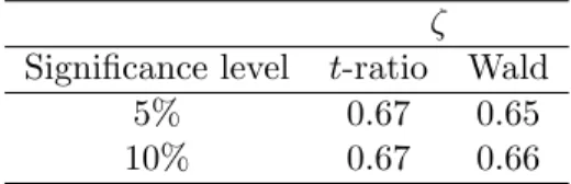
used the same method6 as in Section 3. The rules for the t-ratio and W( 0) based on model (14) with k = 2 are reported in Table 2 below. We report only the rules for thet-ratio and W( 0)because theM Q( ; I)test and the correspondingt-test do not work satisfactorily along with the calibration rules.
Table 2: Calibration Rules for the Centered Subsampling of thet-ratio and Wald test (k= 2)
Signi…cance level t-ratio Wald 5% 0.67 0.65 10% 0.67 0.66
5
Simulation
This section reports empirical size and power of thet-, Wald,Q( 0;1), andM Q( 0; I) tests using subsample critical values. We consider the cases of one and two regressors. The alternative hypothesis is H1 : >0 for the case of a single regressor. That for the case of two regressors is H1 : 6= 0 orH1 : i >0. Data were generated by (1)
and (2) for the univariate case and (14) and (15) for the bivariate case. We set = 0 and = 0 in the data generation because they have no e¤ects on the …nite-sample values of the test statistics. In addition, the elements of in (14) have the same value . Forfuvtg,
uvt iid N(0;1)
was used for the univariate case; and
uvt iid N 0; 1 0:85
0:85 1
for the bivariate case. Note that the elements of uvt are cross-sectionally correlated in the bivariate case. In the data-generating process (15), the diagonal elements of matrix C were set to have the same value denoted by c in subsequent tables. The error terms fuytgwere generated by
uyt= 0uvt+et;
withet iid N(0;1)and = [ ; ]0. Note thatfuvtgand fetgare independent. The
parameter measures the degree of dependence between fuvtg and fuytg.
In the following tables, we considered the casesT = 100, 250, 500;c= 5, 10, 15; = 0, 0.01, 0.05, 0.1; and = 0:5, 1:5, 3.7 We ran 2,000 replications
6We used the data-generating process (DGP) where the covariance between the two innovation
processes for xt is 0.85 and the bivariate vector has the same element c=T. Using more
gen-eral DGPs may yield di¤erent rules, but the di¤erence was not noticeable according to our limited experimentation with di¤erent DGPs.
7Parameter denotes the covariance between
fuytgand fuvtg. The corresponding correlations
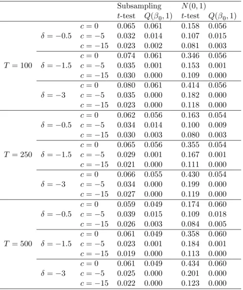
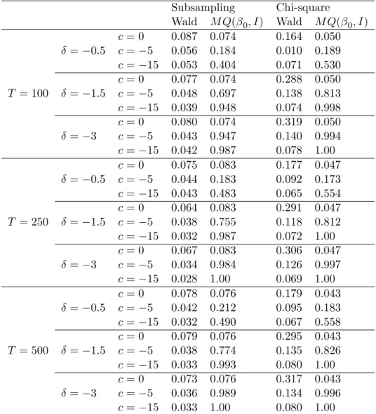
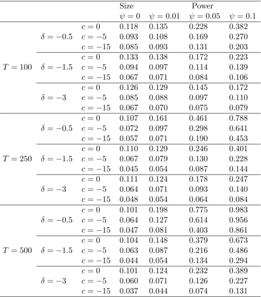
for these tests. Tables 3–5 report the empirical size and power of the t-, Wald,
Q( 0;1), andM Q( 0; I)tests using critical values from the uncentered subsampling with the minimum-volatility rule. Table 3 reports the empirical size and power of the tests for the case of a single regressor. Table 4 reports those of the joint tests for the two-regressor case, while Table 5 reports those of the individual tests. We also report in Tables 3 and 4 the size of the t-, Wald,Q( 0;1), andM Q( 0; I)tests using standard distributions for the purpose of comparison. The results in Tables 3–5 are summarized as follows.
The subsampling-based t- and Wald tests keep nominal size quite well across all values ofT, , and c, though the tests tend to underreject as the value ofc
decreases.
The Q( 0;1) and M Q( 0; I) tests along with subsampling work reasonably well under the null hypothesis when c= 0. However, ascand decrease, their performance deteriorates. Especially when c = 15 and = 3, all the tests are subject to size distortions. An explanation for the poor performance of the tests under the null is provided in Appendix III.
The t- and Wald tests using standard distributions perform poorer as takes smaller values and c is closer to zero. This is well expected from standard theory. Overall, we observe signi…cant advantage of using the subsampling critical values over those from standard distributions.
The Q( 0;1)and M Q( 0; I)tests using standard distributions perform poorly under the null hypothesis unless c = 0. The M Q( 0; I) test shows serious overrejections for c6= 0.
As expected, the power of the tests improves as the value of increases and as
T increases. When = 0:1 and T = 500, the power is close to one in all the cases.
As c takes smaller values, the power of thet- andQ( 0;1)tests in Tables 3–5 tends to decrease. However, that of the M Q( 0;1) tests in Table 4 tends to increase, most likely due to size distortions.
As takes smaller values, the power of the t- and Q( 0;1)tests in Tables 3–5 tends to decrease. By contrast, that of theM Q( 0;1)tests in Table 4 tends to increase, again most likely due to size distortions.
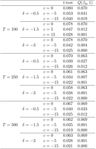
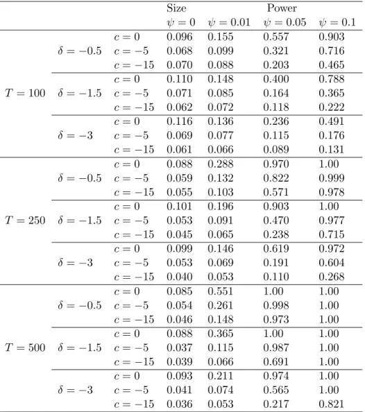
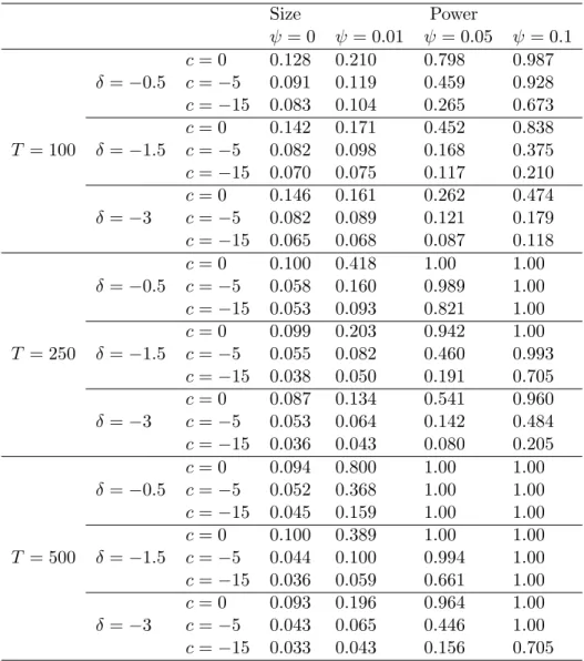
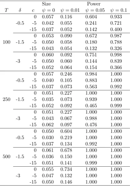
Tables 6–8 report the size and power of thet- and Wald tests using critical values from the centered subsampling with the calibration rules from Tables 1 and 2. The size and power of the Q( 0;1) and M Q( 0; I) tests are not reported because they are unsatisfactory and do not deserve the space. We do not report the results of centered subsampling using the minimum-volatility rule either because these are also quite poor. Tables 6–8 are summarized as follows.
The t-test in Tables 6 and 8 and the Wald test in Table 7 keep nominal size reasonably well when subsampling critical values are used across all values of
T; , and c, though some overrejections are observed when c= 0.
The power of the tests improves as the value of increases and asT increases. In particular, we observe signi…cant power gain over uncentered subsampling. Asc takes smaller values, the power of the tests decreases.
As takes smaller values, the power of the tests tends to decrease.
For comparison, we report the …nite-sample size and power of the Bonferroni t -and Q-tests examined by Campbell and Yogo (2005) in Table 8. Since the tests are designed for the case of a single regressor, the results should be compared to those in Tables 3 and 6. The results in Table 9 are summarized as follows.
Panel A of Table 9 shows that the size properties for both tests are very good. Unlike the subsampling-based tests we consider above, there is no evidence that these Bonferroni tests overreject even whenc= 0.
Panel B shows that the Bonferroni Q-test tends to dominate the Bonferroni
t-test in terms of power which is consistent with the results that Campbell and Yogo report.
Overall, the Bonferroni Q-test appears to be more powerful than univariate centered subsampling reported in Table 6, except whenT and are both small (T = 100, = 0:01).
The results above indicate that the t- and Wald tests along with centered sub-sampling work reasonably well in the case of two regressors and are recommended for empirical applications. When there is only one regressor, the Bonferroni Q-test appears to be the best choice.
6
Testing for stock-market predictability
In this section, we apply the subsampling-based tests developed above to investigate the predictability of stock returns. We use thet- and Wald tests along with centered subsampling in light of the simulation results of the previous section. We …rst consider such predictor variables as the dividend–price ratio, the earnings–price ratio, and the short-term interest rate, which have been widely used in previous studies. In addition to these popular variables, we also consider predictors proposed by more recent theories. In particular, we examine: (1) the consumption–wealth ratio (cay) proposed by Lettau and Ludvigson (2001a, 2001b), (2) the labor-income–consumption ratio (sw) proposed by Santos and Veronesi (2006), (3) the surplus-consumption ratio based on the linear habit speci…cation examined by Li (2001) and others, and (4) the surplus-consumption ratio based on the nonlinear habit speci…cation proposed by Campbell and Cochrane (1999).
The fact that our approach can handle nearly integrated regressors and can be used in a multiple-regression setting allows us to address important economic ques-tions. First, by including both the dividend–price ratio and a second variable as predictors in the predictive regression, we can investigate if the second predictor has predictive power for stock returns beyond that already contained in the dividend– price ratio. In some of the recent studies mentioned above, the authors use standard asymptotics to demonstrate that the predictors suggested by their theories have incre-mental predictive power for stock returns relative to the dividend–price ratio. Since these new predictors and the dividend–price ratio are typically highly persistent, the use of standard asymptotics may not be valid.8 By contrast, since our approach per-forms well even in these cases, we can use it to examine if the new predictors indeed contain incremental information.
Second, some of the predictors mentioned above are closely related and one may be interested in knowing their joint predictive power. For example, we may be in-terested in knowing the joint predictive power of the consumption–wealth ratio cay
and the labor-income–consumption ratiosw as bothcay andsw depend on aggregate consumption and labor income. We can also test for the joint predictive power of di¤erent habit speci…cations. Using the subsampling approach, we can carry out joint tests that are robust to the presence of nearly integrated predictors.
Third, some of the predictors can be viewed as being in competition with each other. For example, Campbell and Cochrane (1999) propose a form of nonlinear habits to overcome certain de…ciencies of the more traditional, linear habit speci…ca-tion. Since higher surplus consumption forecasts lower future returns in both of these models, we can use our subsampling-based tests to see which speci…cation has more predictive power when both predictors are included in the predictive regression.9
Among recent studies, our analysis here is most closely related to the works of Ang and Bekaert (2005) and Campbell and Yogo (2005). Ang and Bekaert examine stock-market predictability in both the univariate and multivariate settings, but their tests are developed for stationary regressors. Campbell and Yogo model regressors as nearly integrated, but their Bonferroni procedure is only applicable to univariate tests. Our tests allow for near unit roots in the regressors and can be used in a multivariate setting.
6.1 Data description
We use the annual, quarterly, and monthly NYSE/AMEX value-weighted index data from the Center for Research in Security Prices (CRSP) to construct series of stock returns and dividend–price ratios at the corresponding frequencies. Since earnings data are not available from CRSP, we construct earnings–price ratios using Standard and Poor’s (S&P) 500 data.
8
Even though some theoretical models suggest that certain predictor variables (such as the dividend–price ratio) are stationary (see Ang and Bekaert 2005, for example, for one such model), empirical tests often cannot reject the hypothesis that those variables contain a unit root.
9Such a comparison is particularly interesting since the results reported by Li (2001) suggest that
We follow Campbell and Shiller (1988) and Campbell and Yogo (2005) in our con-struction of the dividend–price and earnings–price ratios. We compute the dividend– price ratio as dividends over the past year divided by the current price, and the earnings–price ratio as a moving average of earnings over the past ten years divided by the current price.
In our predictability regressions, we forecast the excess returns on stocks over a risk-free rate. We use the one-month and three-month T-bill rates, respectively, for our monthly and quarterly analyses. For annual data, we construct the risk-free return by compounding the returns on the month T-bill. We also use the three-month T-bill rate as a predictor variable in some of our analyses. All T-bill data are obtained from CRSP.
The full sample period is from 1926 to 2004, although we also consider the sub-periods 1926–1994 and 1952–2004. We examine the subperiod 1926–1994 because the valuation ratios we consider have dropped to their lowest levels in history since the late 1990’s, and it is interesting to see if such changes a¤ect our results. For regressions that include the three-month T-bill rate as a predictor variable, we only consider the subperiod 1952–2004. This is because the U.S. Federal Reserve pegged interest rates before the Treasury Accord of 1951, and interest-rate data prior to 1952 are di¢ cult to interpret.
In addition to the dividend–price ratio, the earnings–price ratio, and the three-month T-bill rate, we consider a few consumption-based predictors proposed by recent research. We obtain real per capita consumption of nondurables and services from the Bureau of Economic Analysis (BEA), U.S. Department of Commerce. Our de…nition of labor income follows that in Lettau and Ludvigson (2001a) and Santos and Veronesi (2006). In particular, it is de…ned as wages and salaries plus transfer payments plus other labor income minus personal contributions for social insurance minus taxes. The source of all these series is the BEA. We use an updated series for cay, constructed by Lettau and Ludvigson (2001a, b), from Martin Lettau’s website. The appendix to Lettau and Ludvigson (2001a) details the construction of this variable. Due to data limitation, tests involving the consumption-based predictors are carried out for the subperiod 1952–2004, and at quarterly and annual frequencies only.
6.2 Valuation ratios and the risk-free rate as predictors
We …rst consider tests of stock-return predictability using the dividend–price ratio, the earnings–price ratio, and the three-month T-bill rate as predictor variables. Table 11 reports results of our subsampling-based tests of stock-market predictability. We use centered subsampling where the block size is selected based on a calibration rule. We carry out one-sided tests at the 5% level. Panel A reports results of t-tests in univariate predictions and Panel B reports results of the individual t-tests and joint Wald tests in bivariate predictions.
From Panel A, we see that the strongest evidence for predictability comes from the 1926–1994 subsample. With the exception of the dividend–price ratio at the monthly frequency, the null of no predictability is rejected at the 5% level in all other setups. The evidence for predictability is much weaker for the full sample and for
the 1952–2004 subsample. For the full sample, we …nd that only the earnings–price ratio at the quarterly frequency has signi…cant predictive power at the 5% level. For the 1952–2004 subperiod, only the short-term interest rate at the monthly frequency is signi…cant at 5%.
To compare our results with those reported by Campbell and Yogo (2005), we also carry out our tests for 1926–2002, the period Campbell and Yogo consider. For this period, we …nd that the dividend–price ratio (at the annual frequency) and the earnings–price ratio (at both the quarterly and monthly frequencies) are signi…cant at the 5% level. Overall, our univariate results regarding the predictive power of the two valuation ratios are almost identical to those obtained from the Bonferroni
Q-test that Campbell and Yogo propose; with respect to the short-term interest rate, the BonferroniQ-test …nds evidence for predictability in both quarterly and monthly data, but we …nd such evidence only at the monthly frequency.
Turning to the bivariate results on Panel B, we see evidence of predictability that is more evenly spread out across subsamples. In particular, in the 1952–2004 subperiod, we can now reject the null of no joint predictability for the earnings– price ratio and the short-term interest rate at all three frequencies. In addition, the combination of the dividend–price ratio and the short-term interest rate is also rejected at the monthly frequency. For the other two samples, we …nd evidence of joint predictability for the two valuation ratios at both the monthly frequency (for the 1926–1994 subperiod) and the quarterly frequency (for 1926–1994 and 1926–2004).
Comparing the results on Panels A and B, we see the value of performing joint tests. For example, in the 1952–2004 subsample, even though univariate tests …nd predictability only at the monthly frequency, joint tests uncover predictability at all three frequencies. At the same time, predictor variables that are individually signi…cant in univariate tests do not necessarily become jointly signi…cant; looking at the 1926–1994 subperiod and using annual data, even though the valuation ratios are each individually signi…cant, they are not jointly signi…cant.
Lamont (1998) examines the joint predictive power of the dividend–price ratio and the earnings–price ratio for future stock returns. In particular, he …nds that when both valuation ratios are used as predictors, the dividend–price ratio remains positive and signi…cant, but the earnings–price ratio becomes negative and signi…cant. Since Lamont uses standard asymptotics for inference, but the valuation ratios are highly persistent and strongly correlated with returns, we apply our subsampling-based tests on Lamont’s sample (quarterly Standard & Poor’s Composite Index data from 1947 to 1994) to test his conclusion. As expected, we …nd that the point estimates are the same as those found by Lamont (1998). More importantly, the coe¢ cient on the dividend–price ratio remains positive and signi…cant and that on the earnings–price ratio negative and signi…cant at the 5% level.
However, from the results reported in Table 11, Panel B, we see that Lamont’s (1998) …nding seems to be present only in the most recent sample period. We …nd the same positive–negative pattern on the coe¢ cient estimates for the dividend–price and earnings–price ratios in the 1952–2004 osubperiod only. By contrast, in the 1926– 1994 subperiod and in the full sample, it is the dividend–price ratio (rather than the
earnings–price ratio) that turns negative.
6.3 Consumption-based variables as predictors
One testable implication of consumption-based asset pricing models is that certain state variables implied by theory have predictive power for stock returns. Thus, researchers often use the …nding of predictability as evidence in support of their models. A popular approach is to include both the state variable under consideration and the dividend–price ratio in the predictive regression, and then examine if the state variable has any marginal predictive power beyond that of the dividend–price ratio. Since previous tests are based on standard asymptotic theories, we reexamine their results for robustness using our subsampling-based approach.
The …rst two consumption-based predictor variables we consider are the consump-tion–wealth ratio (cay) proposed by Lettau and Ludvigson (2001a, 2001b) and the labor-income–consumption ratio (sw) proposed by Santos and Veronesi (2006). Both variables depend on aggregate consumption and aggregate labor income.
Table 12 shows that both variables have predictive power for stock returns. Panel A reports results for annual data and Panel B reports results for quarterly data. From rows 1 and 2 of Panel A, we see that bothcayandsw have predictive power for stock returns at the annual frequency beyond that contained in the dividend–price ratio. In row 3 of Panel A, we see that both variables are individually signi…cant in a bivariate predictive regression. This …nding suggests that even though both variables depend on aggregate consumption and labor income, they each contain independent predictive power for stock returns. By examining the corresponding rows on Panel B, we see that the predictive power of sw weakens but that of cay remains. This
result is consistent with the …ndings of Santos and Veronesi (2006), who show that the predictive power ofsw lies in annual and lower frequencies.
We next turn to two habit-based predictors. The …rst is the log surplus con-sumption based on a linear habit, ln(Ct Xlin;t), and the second is the log surplus
consumption based on a nonlinear habit, ln(Ct Xnonlin;t). Xlin;t and Xnonlin;t
de-note the level of linear and nonlinear habit, respectively, and are discussed in detail below. As Campbell and Cochrane (1999) and Li (2001) argue, at times when surplus consumption is low, consumers become conditionally more risk averse and demand a higher expected return on stocks. Campbell and Cochrane rely on calibration re-sults to demonstrate how this negative relationship between surplus consumption and expected stock returns arises. Li uses standard asymptotics to show that this relationship is there in the data as well. In particular, Li examines a wide range of linear habit speci…cations and …nds that some have performance similar to that of Campbell and Cochrane’s (1999) nonlinear speci…cation.
In particular, Li (2001) considers linear habitXlin;t of the form
Xlin;t = 1 'm 1 'J m J X j=1 '(j 1)mCt j;
persistence of the habit, for example, how quickly the e¤ects of past consumption die out. The integerm denotes the number of months elapsed between periodst 1 and t. The integer J 1 measures the duration of the habit, that is, the truncation point beyond which past consumption has no e¤ect. The constant0< <1controls the level of the habit relative to current consumption. We follow Li (2001) in setting = 0:98. Since Li shows that speci…cations with ' 0:99 and J equal to 5 years perform the best, we focus on the case of '= 0:99 and J =20 quarters.
In their nonlinear habit-persistence model, Campbell and Cochrane (1999) do not specify Xnonlin;t directly. Instead, they de…ne the surplus-consumption ratio St Ct Xnonlin;tCt , and postulate that the log surplus-consumption ratio, st, follows a heteroskedastic AR(1) process,
st+1= (1 )s+ st+ (st)(ct+1 ct g);
where ,g, ands are parameters, and ct denoteslnCt. The function (st) controls
the sensitivity of st+1 to contemporaneous consumption. We follow Campbell and Cochrane’s (1999) choice of parameter values and the speci…cation for (st):10 We
assume that s1 is equal its steady state value s. To weaken the dependence of our results on this choice ofs1, we begin our simulation 20 quarters before the start date of our predictive regressions (i.e., we begin our simulation in 1947Q1), so that we can drop the …rst 20 quarters of observations when we examine the predictive power of ln(Ct Xnonlin;t) from 1952Q1 to 2004Q4.
When we include surplus consumption together with the dividend–price ratio in the predictive regression, the coe¢ cients on both the linear and nonlinear speci…ca-tions have the expected negative sign— higher surplus consumption forecasts lower future returns. However, the coe¢ cients tend not to be signi…cant, with the exception of the nonlinear speci…cation ln(Ct Xnonlin;t) at the annual frequency.
The “head-to-head” comparison between ln(Ct Xlin;t) and ln(Ct Xnonlin;t) is more interesting. When we include both surplus-consumption variables in the predic-tive regression, the coe¢ cient on the nonlinear habit remains negapredic-tive and signi…cant, but that on the linear habit turns signi…cantly positive in annual data, and insigni…-cantly positive in quarterly data. Campbell and Cochrane (1999) use simulations to show that their nonlinear habit speci…cation can overcome many di¢ culties that the more traditional, linear speci…cation faces in asset pricing. Here, we show that the nonlinear speci…cation also has superior forecasting power for stock returns.
Finally, we investigate if the habit-based variables— the consumption–wealth ra-tio, cay, and the labor-income–consumption ratio, sw— have the same information
content in terms of stock-return prediction. When we include both cay and ln(Ct Xnonlin;t) in the predictive regression, we see that both variables remain signi…cant
with the expected signs. On the other hand, sw and ln(C
t Xnonlin;t) become
in-dividually insigni…cant, although they are still jointly signi…cant when we carry out
1 0Speci…cally, we assume that = 2, = 0:87,g= 1:89%, and
c= 1:5%, where ,g, and care
annualized values. See Campbell and Cochrane (1999) for a detailed discussion on the speci…cation of (st).
the test at the annual frequency. These results indicate that cay has more incre-mental information than sw does, relative to the information already contained in ln(Ct Xnonlin;t).
7
Conclusion
Many popular stock-return predictor variables are highly persistent. Even though there may be plausible theoretical grounds to assume that some of these variables are stationary, we often cannot empirically reject the notion that these variables contain a unit root. Thus, it is natural to model these predictor variables as being nearly integrated. At the same time, more than one such predictor variable is of interest to …nancial economists. Thus, in testing for stock-return predictability, it is important to be able to carry out tests in a multivariate setting.
Some previous studies on stock-return predictability has modelled the predictor variables as nearly integrated, but their methods are only applicable to univariate regressions. Other studies have examined multivariate forecasts, but the regressors are assumed to be stationary. We add to this literature by proposing a subsampling-based test that can incorporate nearly integrated regressors in a multivariate setting. By avoiding the need to estimate various nuisance parameters (most notably, the degree of persistence of the predictor variables), our subsampling-based approach overcomes the main di¢ culty in extending univariate tests that allow for nearly in-tegrated predictors (such as the Bonferroni tests) to a multivariate setting.
We carry out extensive simulations to demonstrate that our subsampling-based tests have desirable size and power properties. On the other hand, the performance of the conventionalt-tests and Wald tests that use standard asymptotics deteriorate when the persistence of the predictor variables approaches unity. These results in-dicate that conclusions obtained using these tests (such as the …ndings in Ang and Bekaert, 2005) can be misleading if the regressors in question in fact contain near unit roots.
Our subsampling-based tests suggest that the evidence for stock-return predictabil-ity is quite strong when we use valuation ratios and the risk-free rate as predictors. In univariate tests, we …nd that the evidence is more concentrated in the subperiod from 1926–1994. In bivariate tests, we …nd evidence for predictability in the full sample period 1926–2004, and in the subperiods 1926–1994 and 1952–2004. We also demonstrate the value in being able to carry out joint tests— there are numerous cases where univariate tests are insigni…cant but joint tests are not.
We also consider the predictive power of a number of consumption-based vari-ables. We …nd that both the consumption–wealth ratio (cay) proposed by Lettau and Ludvigson (2001a, 2001b) and the labor-income–consumption ratio (sw) proposed by
Santos and Veronesi (2006) have signi…cant marginal information to forecast returns beyond that already contained in the dividend–price ratio. We also see that the information content of these two variables are not the same, as both variables are individually signi…cant in tests using annual data. Between the surplus-consumption variables based on linear and nonlinear habits, we …nd that the nonlinear speci…cation
has stronger predictive power.
There are several directions for further research. Although we have examined a number of consumption-based models in this study, we have not considered models that explicitly take housing or durables consumption into account. Lustig and Van Nieuwerburgh (2005), Piazzesi et al. (2006), and Yogo (2006) show that these models have desirable asset pricing implications. It would be interesting to compare these models’time-series predictive power for stock returns. Second, although it is easy to see that our theory applies to more than two regressors and to forecast horizons longer than the annual frequency, we have to carry out further simulations to investigate the performance of our tests in such cases.
Appendix I: The main theoretical results
This appendix proves that the subsampling approach provides valid approximations to the limiting distributions oft( 0)andQ( 0;1)de…ned by (4) and (6), respectively. A major source of complication for the proof of the following theorem is that t( 0) and Q( 0;1) are not identically distributed when they use blocks of data starting froms. This follows because the test statistics depend onvs 1 which is not identically distributed for eachs. However, since the initial variablevs 1 does a¤ect the limiting distributions of the test statistics asb! 1, they are identically distributed for large
b which makes the following theorem hold true.
Theorem A.1 Let b = O(T ) with 12 < 23. Denote the limiting distribution functions of t( 0) and Q( 0;1) as Jt( ) and JQ( ), respectively. Suppose that ut =
(uvt; et)0 satis…es Assumption 1. Then,
(i) supx2RjLzT(x) Jz(x)j!p 0 (z=t; Q) asT ! 1;
(ii) For 2(0;1), let cz
T(1 ) = inffx : LzT(x) 1 g and cz(1 ) = fx :Jz(x) = 1 g. Then,
czT(1 )!p cz(1 ) as T ! 1:
Proof. (i) We will prove the results only for Q( 0;1)because those for t( 0) can be proven in the same way. Consider b;s=Qb;s( 0;1)jvs 1=0, which is the test statistic
Qb;s( 0;1)conditional on the restriction vs 1 = 0. The empirical distribution func-tion using b;sis written asMT(x) = T 1b+1PTs=1b+11f b;s xg. Becausef(uvt; et)0g
is strictly stationary and because b;sis a measurable function of only fetgst=+sb+11 and
fuvtgts=+sb 2 due to the conditioning vs 1 = 0, b;s has the same distribution for each sand b. Thus, we may write
MT(x) JQ(x) 1 T b+ 1 TXb+1 s=1 (1f b;s xg E1f b;1 xg) + E1f b;1 xg JQ(x) = AT(x) +BT(x); say:
Since 1f b;s xg is a measurable function of fetgts=+sb+11 and fuvtgst=+sb 2, the law of
large numbers for mixing processes stated in Lemma A.3 yieldsAT(x) a:s:
! 0for each
x2R. From this follows supx2RAT(x) a:s:
! 0 due to Lemma A.4. In addition,BT(x)
converges to zero uniformly in x since E1f b;1 xg !JQ(x) for eachx and JQ( ) is a continuous function (see Lemma 3 of Chow and Teicher, 1988, p.265). Thus, we have proven that
sup
x2R
MT(x) JQ(x) a:s:! 0: (A.1)
In order to prove a similar result for LQT( ), consider an inequality
sup x2R LQT(x) JQ(x) sup x2R LQT(x) MT(x) + sup x2R MT(x) JQ(x) :
The second term on the right-hand side of this inequality has been shown to be
oa:s:(1). In order to show that the …rst term is negligible in probability, assume that Qb;s( 0;1) = b;s+ T bs (A.2)
where
max
s j T bsj=op(1): (A.3)
Then, letting&T b= maxsj T bsj,
sup x2R LQT(x) MT(x) = sup x2R 1 T b+ 1 TXb+1 s=1 (1fQb;s( 0;1) xg 1f b;s xg) sup x2R 1 T b+ 1 TXb+1 s=1 (1f b;s x+&T bg 1f b;s xg) sup x2R
MT(x+&T b) JQ(x+&T b) + sup x2R
JQ(x+&T b) JQ(x)
+ sup
x2R
MT(x) JQ(x) :
Using (A.1) and (A.3), we …nd that the …rst and third terms in the last inequality converge to zero in probability. The second term also converges to zero in probability sinceJQ( )is continuous. Thus, the proof will be complete if relations (A.2) and (A.3) are shown to hold. These are proven in Lemma A.5, so the stated result follows. (ii) Since Lz
T( ) and Jz( ) are nondecreasing functions and Jz( ) is continuous, the
result follows from part (i) and Lemma A.6 in Appendix II. Let LtT(x) = 1 T b+ 1 TXb+1 s=1 1ftb;s(^) xg and LQT (x) = 1 T b+ 1 TXb+1 s=1 1fQb;s(~;1) xg;
wheretb;s(^)and Qb;s(~;1)are de…ned by (10) and (11), respectively. The following
theorem states that the empirical distribution functions, LtT(x) and LQT (x), provide valid approximations to the limiting distributions oft( 0)and Q( 0;1), respectively.
Theorem A.2 Suppose that the same assumptions for Theorem A.1 hold. Then, (i) supx2RjLTz(x) Jz(x)j!p 0 (z=t; Q) as T ! 1;
(ii) For 2(0;1), let cTz(1 ) = inffx :LTz(x) 1 g and cz(1 ) =fx:Jz(x) = 1 g. Then,
cTz(1 )!p cz(1 ) as T ! 1:
Proof. (i) We prove the results only forLtT(x). Using relation (12), write
LtT(x) = 1 T b+ 1 TXb+1 s=1 1ftb;s( 0) + b;s;n xg; where b;s;T = Tb r T(^ 0) ^b;s;y2 Pts=+sb+11(xt 1 x 1;b;s) 2 =b2 1
. We deduce from this relation
that for " >0
LtT(x ")1fETg LtT(x)1fETg LtT(x+"); (A.4) where 1fETg is the indicator of the event fj b;s;T j "g. Since the event En holds with probability approaching one asT goes to in…nity, (A.4) implies that the relation
LtT(x ") LtT(x) LtT(x+") holds with probability tending to one. Because
LtT(x ") Jt(x) LtT(x) Jt(x) LtT(x+") Jt(x); we have sup x2Rj LtT(x) Jt(x)j max sup x2Rj LtT(x+") Jt(x)j; sup x2Rj LtT(x+") Jt(x)j :
Thus, we obtain the stated result by sending " ! 0 and using part (i) of Theorem A.1.
(ii) This follows as in the proof of part (ii) of Theorem A.1.
Appendix II: Technical lemmas
This appendix collects some technical lemmas used to prove Theorem A.1. The …rst result we require is the strong law of large numbers for the function of mixing processes with the number of arguments growing with the sample size.
Lemma A.3 Let Ys = g(zs; zs+1; : : : ; zs+b), where b is an integer satisfying b = O(T ) with 0< <1. Suppose for some constants c and dthat
(a)sups 1kYsk2+"< c <1 for " >0;
(b)fzsg is strong mixing with its mixing coe¢ cients z;m satisfying, for >0,
1 X m=1 =(2+ ) z;m <1: Let ST b=PTs=1b(Ys E(Ys)). Then, as T ! 1, 1 T bST b a:s: !0:
Proof. See Lemma A.2 of Choi and Chue (2004).
The following lemma, taken from Davidson (1994, p. 332), states that the point-wise a.s. convergence of the empirical distribution function is su¢ cient for the Glivenko–Cantelli lemma. Davidson states the lemma for iid random variables, but its use for dependent random variables is easily veri…ed as long as the pointwise strong law of large numbers holds for them.
Lemma A.4 For a set of random variables fY1(!); : : : ; YT(!)g de…ned on the prob-ability space ( ;F; P), de…ne the empirical distribution function as
FT(x) = 1 T T X t=1 1fYt(!) xg: If FT(x) a:s:
! F(x) pointwise for x2R as T ! 1, then
sup
x2Rj
FT(x) F(x)j a:s:
! 0 asT ! 1:
In the following lemma, we prove relation (A.3) to support the proof of Theorem A.1 in Appendix I. The test statistic Qb;s( 0;1)can be written as
Qb;s( 0;1) = g Ps+b 1 t=s+1(vt 1 v 1;b;s) 2 b2 ; Ps+b 1 t=s+1(vt 1 v 1;b;s) ( vt v) b3=2 ; Ps+b 1 t=s+1 vt v 2 b ; Ps+b 1 t=s+1(vt 1 v 1;b;s)et b ; Ps+b 1 t=s+1 vt v et b1=2 ; Ps+b 1 t=s+1e2t b ! ;
where g( ) is a continuous function, v 1;b;s =
Ps+b 1 t=s+1vt 1 b 1 and v = Ps+b 1 t=s+1 vt b 1 . Let
terms involving initial valuevs 1, we obtain Qb;s( 0;1) (A.5) = h vs2 1 Ps+b 1 t=s+1 t s b 2 b2 ; vs 1 Ps+b 1 t=s+1 t s b wt 1 b2 ; vs2 1( 1) Ps+b 1 t=s+1 t s b 2 b3=2 ; vs 1 Ps+b 1 t=s+1 t s b uvt b3=2 ; vs 1 ( 1)Pst=+sb+11 t s b wt 1 b3=2 ; v 2 s 1 ( 1)2Pst=+sb+11 t s b 2 b ; vs 1 ( 1)Pst=+sb+11 t s b uvt b ; vs 1 ( 1)2Pst=+sb+11 t s b wt 1 b ; vs 1 Ps+b 1 t=s+1 t s b et b ; vs 1 ( 1)Pst=+sb+11 t s b et b1=2 ; rb;s ! ; where b = Ps+b 1 t=s+1 t s
b 1 . In relation (A.5),rb;s denotes a vector of terms that do not involvevs 1, These are functions of only fetgst=+sb+11 and fuvtgst=+sb 2 and areOp(1).
Lemma A.5 Let b = O(T ) with 12 < 23. Then, Qb;s( 0;1) = b;s+ T bs and
Proof. A Taylor expansion of (A.5) gives b;s = h(0; : : : ;0; rb;s) +@h @x1jx1=x1 vs 1 T1=2 2 T b2 s+Xb 1 t=s+1 t s b 2 (A.6) +@h @x2jx 2=x2 vs 1 T1=2 T1=2 b Ps+b 1 t=s+1 t s b wt 1 b +@h @x3jx 3=x3 vs 1 T1=2 2 T b3=2( 1) s+Xb 1 t=s+1 t s b 2 +@h @x4jx4=x4 vs 1 T1=2 T1=2 b3=2 s+Xb 1 t=s+1 t s b uvt +@h @x5jx5=x5 vs 1 T1=2 T1=2 b1=2( 1) Ps+b 1 t=s+1 t s b wt 1 b +@h @x6jx6=x6 vs 1 T1=2 2 T b( 1) 2 s+Xb 1 t=s+1 t s b 2 +@h @x7jx7=x7 vs 1 T1=2 T1=2 b ( 1) s+Xb 1 t=s+1 t s b uvt +@h @x8jx8=x8 vs 1 T1=2T 1=2( 1)2 Ps+b 1 t=s+1 t s b wt 1 b +@h @x8jx9=x9 vs 1 T1=2 T1=2 b s+Xb 1 t=s+1 t s b et +@h @x9jx10=x10 vs 1 T1=2 T1=2 b1=2 ( 1) s+Xb 1 t=s+1 t s b et;
where xi denotes thei-th argument of function h( ) and xi lies on the line joining 0
and xi. Obviously, h(0; : : : ;0; zb;s) = b;s. Thus, we need to show that the second to
eleventh terms on the right-hand side of equation (A.6) are op(1). Due to the weak
convergence results for nearlyI(1)processes (cf. Phillips, 1988),
max
s
vs 1
In addition, s+Xb 1 t=s+1 t s b 2 = b 1 X t=1 ect=T 1 b 1 b 1 X t=1 ect=T !2 = b 1 X t=1 1 +ct T +atT 1 b 1 b 1 X t=1 1 +ct T +atT !2 = b 1 X t=1 ct T 1 b 1 b 1 X t=1 ct T !2 +o(1) = c 2 T2 b 1 X t=1 t 1 b 1 b 1 X t=1 t !2 +o(1) = O(b 3 T2); (A.8)
which shows that Pst=+sb+11 t s b 2 is bounded in the limit due to the given as-sumption on b. Moreover, using the strong mixing inequality11 for fetg, we obtain
for a constant C V ar b 1 X t=1 t b et ! (A.9) = 2y b 1 X t=1 ( t b)2+ 2 b 2 X m=1 b 1 X t=m+1 ( t b)( t m b) m 2 y b 1 X t=1 ( t b)2+ 2C b 2 X m=1 =(2+ ) m b 1 X t=m+1 t b t m b 2 y b 1 X t=1 ( t b)2+ 2C b 2 X m=1 =(2+ ) m v u u t Xb 1 t=m+1 ( t b)2 v u u t Xb 1 t=m+1 ( t m b)2 2 y b 1 X t=1 ( t b)2+ 2C b 1 X t=1 t b 2 !b 2 X m=1 =(2+ ) m =O(1);
where Cov(et; et m) = m. The …rst inequality in (A.9) uses the strong mixing
inequality, and the second uses the Cauchy–Schwarz inequality. The last equality is based on (A.8). Relation (A.9) implies that
s+Xb 1
t=s+1
t s
b et=Op(1) (A.10)
1 1The inequality is
jCov(uyt; uy;t+m)j 2(21 1=(2+ )+ 1) u;m=(2+ )kuytk2+ kuy;t+mk2+. For this,
Likewise,
s+Xb 1
t=s+1
t s
b uvt=Op(1) (A.11)
Furthermore, using maxs+1 t s+b 1 wtb1=21 =Op(1)and relation (A.8), we obtain
Ps+b 1 t=s+1 t s b wt 1 b max s+1 t s+b 1 wt 1 b1=2 Ps+b 1 t=s+1 t s b b1=2 max s+1 t s+b 1 wt 1 b1=2 v u u ts+Xb 1 t=s+1 ( t s b)2 =Op(1): (A.12)
Note that the second inequality of (A.12) uses the Cauchy–Schwarz inequality. Since 1 =O(T1)and @xi@h
jxi=op(1) =Op(1) fori= 1; : : : ;9, relations (A.7), (A.8), (A.10) and (A.11) imply that the second to eleventh terms on the right-hand side of equation (A.6) are op(1)uniformly in sas required. This completes the proof.
The following lemma is used to prove part (ii) of Theorem A.1.
Lemma A.6 Let Hn (y) = inffx : Hn(x) yg and H (y) = inffx :H(x) yg. If (a) Hn( ) and H( ) are nondecreasing functions, (b) H( ) is continuous, and (c)
supx2RjHn(x) H(x)j p
! 0 as n ! 1, then Hn (y) !p H (y) for any y 2 R as n! 1.
Proof. Let g(x) =H(x) + supx2Rj n(x)jand f(x) =H(x) supx2Rj n(x)j, where n(x) =Hn(x) H(x). Functionsg( )andf( )are continuous inxand nondecreasing
with probability one. Thus, for y2R, we have with probability one
f (y) H (y) g (y) and f (y) Hn (y) g (y); which imply jHn (y) H (y)j g (y) f (y): Since supx2Rj n(x)j p
! 0, g (y) f (y) !p 0 as n ! 1, from which follows the stated result.
Appendix III: Why does subsampling perform poorly for
the
Q
(
0;
1
)
test?
When c 6= 0, the simulation results in Section 5 indicate that subsampling does not work well for theQ( 0;1)test. This section tries to explain this. To this end, consider
the empirical distribution function LT(x) = 1 T b+ 1 TXb+1 s=1 1f b;s xg;
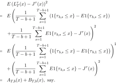
where b;s is either tb;s( 0) or Qb;s( 0;1). The limiting distribution function of T;1 is denoted byJ ( ). The mean-squared error ofLT(x) in estimatingJ(x) is given by
E(LT(x) J (x))2 = E 1 T b+ 1 TXb+1 s=1 (1f b;s xg E1f b;s xg) + 1 T b+ 1 TXb+1 s=1 E1f b;s xg J (x) !2 = E 1 T b+ 1 TXb+1 s=1 1f b;s xg E1f b;1 xg !2 + 1 T b+ 1 TXb+1 s=1 E1f b;s xg J (x) !2 = AT;b(x) +BT;b(x); say:
If b=T !0 and Assumption 1 holds, it can be shown that AT;b(x) = o(1). Thus, it
is the squared bias, BT;b(x), that is asymptotically equivalent to the mean-squared
error. In Table 13, we calculated the mean-squared error and the squared bias using the same data-generating scheme as for Table 3 with T = 250,c= 5, = 3 and
b = 15;27. We chose x such that J (x) = 0:95. Table 13 shows that the Q( 0;1) test has much higher mean-squared error and squared bias than the t-test, which implies that the subsampling critical values for theQ( 0;1)test are unlikely to be as accurate as those for thet-test in estimating its limiting critical values. This explains why the Q( 0;1)test does not perform well in …nite samples relative to the t-test. Obviously, the culprit is its bias. Since T 1b+1PTs=1b+1E1f b;s xg 'Pf b;1 xg for largeb, the substantial bias results from the slow convergence of theQ( 0;1)test to its limiting distribution.12
Table 13: Mean squared error and squared biases of the t- and Q( 0;1)tests
Notes: 1. Data were generated byyt = xt 1+uyt; = 0;xt = exp( T5)xt 1+uvt; uyt =
3uvt+et;uvt iid N(0;1); et iid N(0;1);:T = 250. 2. Block sizes correspond toT0:5andT0:6.
3. uncentered subsampling was used. 4. Results are based on 2,000 replications.
t-test Q( 0;1) MSE Bias2 MSE Bias2
b= 15 0.0166 0.0140 0.9022 0.9022
b= 27 0.0144 0.0099 0.9025 0.9025
1 2We performed the same experiment with larger sample sizes and c= 15. TheQ(
0;1) test
References
Andrews, D.W.K. (1991): “Heteroskedasticity and autocorrelation consistent co-variance matrix estimation,”Econometrica 59, 817–858.
Ang, A. and G. Bekaert (2005): “Stock return predictability: is it there?” Mimeo, Columbia University.
Basawa, I.V., A.K. Mallik, W.P. McCormick, J.H. Reeves, and R.L. Taylor (1991): “Bootstrap test of signi…cance and sequential bootstrap estimation for unstable …rst order autoregressive processes,”Communications in Statistical Theory and Methods 20, 1015–1026.
Bobkoski, M.J. (1983): Hypothesis Testing in Nonstationary Time Series. Ph.D. Thesis, University of Wisconsin, Department of Statistics.
Campbell, J.Y. (1987): “Stock returns and the term structure,”Journal of Financial Economics 18, 373–399.
Campbell, J.Y. and J.H. Cochrane (1999): “By force of habit: a consumption-based explanation of aggregate stock market behavior,”Journal of Political Economy
107, 205–251.
Campbell, J.Y. and R.J. Shiller (1988): “Stock prices, earnings, and expected divi-dends,”Journal of Finance 43, 661–676.
Campbell, J.Y. and M. Yogo (2005): “E¢ cient tests of stock return predictabil-ity,”Journal of Financial Economics, forthcoming.
Chan, N.H. and C.Z. Wei (1987): “Asymptotic inference for nearly nonstationary AR(1) processes,”Annals of Statistics 15, 1050–1063
Choi, I. (2005a): “Inconsistency of bootstrap for nonstationary, vector autoregres-sive processes,”Statistics and Probability Letters 75, 39–48.
Choi, I. (2005b): “Subsampling vector autoregressive tests of linear constraints,”
Journal of Econometrics 124, 55–89.
Choi, I. and T.K. Chue (2004): “Subsampling hypothesis tests for nonstationary panels with applications to exchange rates and stock prices,”Journal of Applied Econometrics, forthcoming.
Chow, Y.S. and H. Teicher (1988): Probability Theory: Independence, Interchange-ability and Martingales. Springer–Verlag, New York.
Datta, S. (1996): “On asymptotic properties of bootstrap for AR(1) processes,”
Journal of Statistical Planning and Inference 53, 361–374.