Ciência e Natura, v. 37 Part 2 2015, p. 328−333
ISSN impressa: 0100-8307 ISSN on-line: 2179-460X
Parallel Genetic Algorithm for Shortest Path Routing Problem with
Collaborative Neighbors
Reza Roshani 1, Mohammad Karim Sohrabi 2
1Department of Computer Engineering, Islamic Azad University, Semnan Branch, Semnan, Iran 2Department of Computer Engineering, Islamic Azad University, Semnan Branch, Semnan, Iran
Abstract
Shortest path routing is generally known as a kind of routing widely availed in computer networks nowadays. Although advantageous algorithms exist for finding the shortest path, however alternative methods may have their own supremacy. In this paper, para llel genetic algorithm for finding the shortest path routing is resorted to. In order to improve the computation time in this routing algorithm and to distribute the load balance between the processors as well, Fine-Grained parallel GA model is opted for. The proposed algorithm was simulated on Wraparound Mesh network topologies in different sizes. To this end, several experiments were anchored to identify the most influential parameters such as Migration rate, Mutation rate, and Crossover rate. The simulation result shows that best result of mutation rate is: about 0.02 and 0.03, and migration rate for transmission to the neighbor’s node is 3 of the best chromosomes. This study has already shown that through using performance-based GA which uses fine-grained parallel algorithms, timing germane shortest path routing can be improved.
Keywords: Parallel Genetic Algorithm, Fine-Grained, Genetic Algorithms, Parallel Communication Topology, Shortest path routing.
1 Introduction
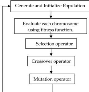
outing in computer network essentially refers to finding a route from source node all way through to the destination node. According to the network, there is a probability that there might be more than one route to be take (Cherkassky, Goldberg, & Radzik, 1996). The task of routing algorithms is originally to come up with the shortest path among the existing routes. Nowadays in computer network realm, usually the shortest path routing algorithms, better known as Dijkstra and Bellman-Ford are rather used (J. F. Kurose, K. W. Ross, 2010). Although the extant algorithms for the shortest path routing have been well established, yet, researchers continue trying to find an alternative method to end up with alternative shortest paths. These alternative methods are usually AI techniques such as (Yussof, Razali, & See, 2011): genetic algorithms, neural networks, particle swarm optimization, ant colony optimization, simulated annealing algorithm, and A* search algorithm. Genetic Algorithms (GA) as the most well-known evolutionary algorithm (Ashlock, 2006) is in fact a multi-purpose search and optimization algorithm inspired by the theory of natural selection and genetics (Goldberg, 1989). Genetic algorithms using encoded chromosomes try to bring forth a solution for this problem. Each chromosome is composed of several genes. The solution for the problem is provided based on group chromosome that represents a population per se. For each iteration in the algorithm, one or more genetic operations on population of chromosome are executed such as: crossover and mutation which altogether these results of genetic operation make up the next generation of solutions. This process continues until a solution is found or rather a terminate condition occurs. The main idea of GA is that population chromosome tends to converge slowly toward good response. Outline genetic algorithm is shown in Figure 1.
One of the latest proposed algorithms for shortest path routing based on GA is proposed by Salman and colleagues, in which
coarse-grained parallel model are implemented upon Waxman and Mesh network. In this article fine-grained parallel model in order for optimal use
and load balancing distribution among
processors are resorted to. In fact, in this paper a fine-grained parallel genetic algorithm using neighborhood techniques for shortest path routing problem is provided. Main goal of this paper is to improve computation time by running parallel GA. The proposed algorithm was implemented in Visual C#.Net 2013 and MPI messaging passing interface.
Figure 1: General Genetic Algorithm Model
2
Parallel Genetic Algorithms
With larger and more complex problem, the response time for GA increases proportionately. Thus to speed up genetic algorithm, we’d rather implement them in parallel. Fortunately GA works on a population of independent solutions, which allows distribute computational load on multiple processors. However, the problem needs to have the ability to be implemented in parallel. In general, there are four models for the implementation of parallel genetic algorithms as proceeds (Cantú-Paz, 1998), (Shahhoseini, Mousavi Mirkalayy, & Mollajafari, 2012):
Master-Slave Model: In this model, a computing node is considered as Master Node and the other are namely affiliated as servants of
R
Generate and Initialize Population
Evaluate each chromosome using fitness function.
Crossover operator Selection operator
the Manager Node. The Manager Node has the population and many GA Operations in control. The Manager can assign one or more computing complex works to servants. Through this course, sending one or more chromosomes from server to servants is practiced. Then manager waits until the results return back by servants.
Coarse–Grained Model: In coarse-grained GA, the population is divided among computing nodes and each node applies GA operation on its subpopulation. To ensure, good solutions will be distributed to other nodes, sometimes nodes can exchange their chromosomes, with certain rate of
probability. This exchange operation is
essentially called Migration, which in fact stands for sending a chromosome from one node to other nodes. After receiving chromosome the nodes can replace yet another chromosome in the population, but which chromosome is selected for migration or replacement depends on the migration strategy that was earlier used.
Fine–Grained Model: This model enjoys the highest level of parallelism among the other four types of parallel GA. Typically; nodes are placed in a spatial structure where each node is connected to only the neighboring nodes. Population is rather known as a set of the chromosomes of nodes. Also in this model, the overlay neighbors are used to spread the good characteristics of a chromosome across the total population. The fine-grained GA is running according to the interactions among the nodes, so the overhead communication is definitely high.
Hierarchical Model: This model is also called hybrid model, which is composed of two levels, higher level algorithm acts as a coarse–grained GA and in the lower level it just acts as a fine– grained GA.
3 Parallel Communication Topology
Topology is originally a criterion for the classification of the communication network across multi-processor systems. Topology is tasked to determine how to connect processors and memory. Topology in parallel algorithms is similarly assigned to determine how to connect processors and memory to other processors and memory. For example in a fully connected topology, each processor is connected to all available processors in the computer system.
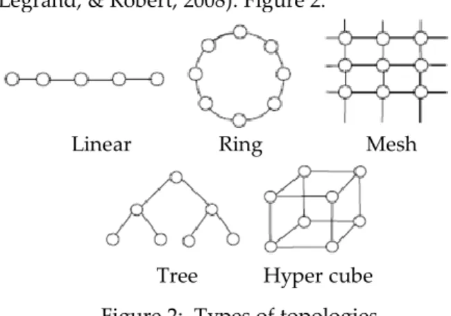
In general, topology can be bifurcated into two groups: static and dynamic. In static networks all connections are created right at the design time. But in dynamic networks, as necessity rises, connections between two or more processors are made. Different types of Static topology are but no limited to: linear,
ring, mesh, tree, hypercube (Casanova,
Legrand, & Robert, 2008). Figure 2.
Linear Ring Mesh
Tree Hyper cube
Figure 2: Types of topologies
The researchers in this paper used wraparound Mesh topology for all nodes in that
the number for all neighbors and
communications were identical. The model is as put on display in Figure 3.
Figure 3: Wraparound Mesh
In this topology, all nodes communicated only with their neighbors. As seen, the extreme nodes are connected to the other side nodes; this connection repeats for the same number of neighbors for all the nodes.
4 The Proposed algorithm
The proposed algorithm uses fine-grained model in parallel GA, the main reason for choosing this is the high level of corporation in this model. The implementation of parallel GA makes all computational nodes generate their sub-population randomly and apply GA operations respectively. Finally, after the execution of iteration for each node, they send
“achieved finest path” to their neighbor’s nodes and receive “finest paths” from neighbor’s path in return and substitute them for their worst paths. Operation of computing nodes is enumerated as follows:
1. Generate subpopulation randomly.
2. Calculating fitness of each chromosome in subpopulation.
3. Identify Neighbors.
4. Send the best chromosome to neighbors. 5. Receive the best chromosome from neighbors. 6. Execute several Crossover operations over time mainly to generate new children of subpopulation, Parent chromosomes are randomly selected from the subpopulation. 7. Execute mutation operation on chromosomes. 8. Migrate is to receive 3 best chromosome and
replace 3 worst chromosome in
subpopulation.
9. Repeat step 2, until sub-population converges or the maximum iterate of steps is obtained the answer, we got maximum iterate 50.
4.1 Display path in Genetic Algorithms
A network can be displayed as a directed graph G (V, E) as it is in figure 4, where in V as a set of nodes represents routers and E is better known as a set of connected edges among the routers. Any edge (i,j) with an integer represents the cost of sending data from node i to node j and vice-versa.
Figure 4: Directed Graph
In the proposed algorithm, any of the chromosomes is encoded as a set of node identifiers which is located somewhere ranging from source up to destination. To wit, the first gene in chromosome is always labeled as source node and the destination node is the last. Since different paths may involve different number of intermediate nodes, so chromosomes length varies. Repeating a node among chromosomes represents a loop in the path, which should be removed.
4.2 Generate Population
In the beginning, sub-population should be created by means of those chromosomes which stand for random paths. Although paths are random, they are still assumed to be valid. Chromosome is essentially considered as a sequence of extant nodes throughout source and destination path. Sn represents the number of generated chromosome for each sub-population; this in fact depends on the size of total population and number of computing nodes, as shown in equation (1).
(1)
Sn represents sub-population of nth node; P represents total size of population and N is the count of nodes. The algorithms which were availed to generate random paths are as follows: 1. Start from source node.
2. Generate unvisited list, at first, this list includes all nodes except the source node and once the node is already selected, its value will be removed from the unvisited list. 3. Randomly select one node from the unvisited
list and remove the selected node from the list. Removing a node from the list is done just by moving a pointer.
4. If the selected node is in connection to the current node, this node is considered as the next one in the path and with the new node will be looking for the other node (Go to stage 3), Otherwise it will be looking for the other node with the previous node (Go to stage 3). 5. If the unvisited list length is 0 then go to stage
1.
6. Repeat until the destination node is found.
4.3 Fitness function
Each chromosome in the population has a fitness value which is calculated by means of the fitness function, this value represents the proportion of the suitability of each solution of the chromosomes, and this information is used to generate chromosomes in the next iteration. In the proposed algorithm fitness function is defined as follows:
fi represents the fitness value of ith chromosome, and Pi represents the total cost of path it chromosome. In this manner fitness function gives greater value for shorter paths.
4.4 Selection function
This function is used to select a chromosome for crossover and mutation. Selection for crossover operation is basically meant for choosing two chromosomes with higher fitness in the population as the parent. Selection for mutation and crossover operations occurs mostly after 0.5% of the population. For example, if population size is 1000, selection is somewhat between 5th to 1000th chromosomes. Since the beginning of the population includes the best chromosomes and it is rational not to lose their negative genetic operation, so only some first chromosomes are not selected for changes (genetic operation). Chromosomes with a positive change can be placed in front the population.
4.5 Crossover function
Crossover of the two parent chromosomes were adopted through selection function. To ensure that the generated path by crossover operator still sounds valid it is required that two chromosomes be chosen which are common in at least one node (other than source and destination nodes). If the two extant chromosomes are sharing commonality in more than one node, then one node which is randomly selected is called crossover point. As a case in point, suppose there are two chromosomes as follows: Selected chromosome 1: [A B C G H I X Y Z] Selected chromosome 2: [A K L M I T U Z]
A and Z represent the source and the destination nodes respectively. In this example I is a common node. So the crossover operation changes the first part of chromosome 1 as well as the second part of chromosome 2, and vice versa; which are realized into two new members of chromosomes in the population. The result of crossover is child chromosome as follows: First chromosome: [A B C G H I T U Z] Second chromosome: [A K L M I X Y Z]
4.6 Mutation function
Selection of each chromosome through crossover operation leaves little chance for change; no surprise the mutation operation is preferred. Mutation probability is shown with the Pm, for all tests Pm is ranging from 0.02 to 0.03.Hence for each selected chromosome in the mutation operation, a random mutation point is selected. Then the chromosomes undergo changes from the mutation point onward. For example, suppose that the chromosome selected for mutation operation is as the example:
Selected :[A C E F G H I J K L M N Y Z]
A and Z are respectively the sending and receiving nodes. Suppose that the node I is selected as a mutation point. Then the mutated chromosome is similar to the following:
Mutated: [A C E F G H I x1 x2 x3 … Z]
The mutated chromosome includes a new path from I to Z, where Xi represents the ith node in
the new path. The new path is created in the same way as to the randomly created initial population.
4.7 Migration
Migration is a genetic action which is mostly availed in parallel genetic algorithms. Each computing node develops its subpopulations independently. Migration is an action that is used to increase the diversity of the population of each computing nodes. In fact, migration denotes sending chromosome from each computing node to yet another computing node. Besides, each of the computing nodes receives migrated chromosome from other computing nodes. The received chromosome can be replaced by one of the sub-populations chromosomes. There are several strategies for migration, in which any computing node can send the best chromosome or the random chromosome to other nodes from the sub-population. On the other side, it can be replaced by the worst chromosomes or random chromosome in the population. The migration strategy that was used for the algorithm was to send the best chromosome and replacement by the worst chromosome.
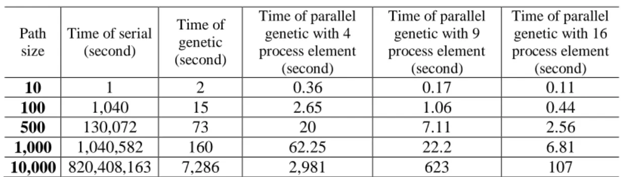
The proposed algorithm was implemented in the Visual studio.NET 2013 environment and in C# programming language on a computer featured as Windows 7 x64 equipped with the processor Intel 2.8GHz core2 Quad and RAM 8GB and run on MPI with 4, 9 and 16 process
element. This simulation was performed on a wraparound mesh topology and length of paths were considered as 10, 100, 500, 1000 and 10000. The results of the implementation of the algorithm are shown in Table 1.
Table 1: Time of algorithms for finding shortest path problem
Path size Time of serial (second) Time of genetic (second) Time of parallel genetic with 4 process element (second) Time of parallel genetic with 9 process element (second) Time of parallel genetic with 16 process element (second) 10 1 2 0.36 0.17 0.11 100 1,040 15 2.65 1.06 0.44 500 130,072 73 20 7.11 2.56 1,000 1,040,582 160 62.25 22.2 6.81 10,000 820,408,163 7,286 2,981 623 107
Several experiments were performed to identify the most influential parameters such as Migration rate, Mutation rate, and Crossover rate. The best result of mutation rate was drawn
as about 0.02 and 0.03, and the migration rate was 3 best chromosomes for sending to the neighbors’ nodes.
6 Conclusion
Routing is one of the major fields of computer networks. According to the algorithms and techniques that were presented in this field, in this study, an algorithm was proposed which used parallel genetic algorithm for obtaining the shortest path among the available paths at the right time. The fine-grained parallel genetic algorithm model is used so that we can take
maximum benefit from parallelism. To
implement parallelism, multi computing nodes with wraparound mesh topology was used. Hence each computing node generated its own sub-population through parallelism at the same time. Then genetic operators were applied to evaluate subpopulation chromosome and then it sent 3 best chromosomes for other computing nodes according to network topology that ultimately replaced the worst chromosome in sub-population. This process was repeated until the algorithm managed to archive the result. The proposed method in genetic algorithm and parallel genetic algorithm were compared with the serial algorithm. The experiment showed that the proposed method obtained the result in an apt moment.
References
Ashlock, D. (2006). Evolutionary Computation for Modeling and Optimization. Springer Science & Business Media.
Cantú-Paz, E. (1998). A survey of parallel genetic algorithms. Calculateurs paralleles, reseaux et systems repartis, 10(2), 141-171.
Casanova, H., Legrand, A., & Robert, Y. (2008). Parallel Algorithms. CRC Press.
Cherkassky, B. V., Goldberg, A. V., & Radzik, T. (1996). Shortest paths algorithms: theory and
experimental evaluation. Mathematical
Programming, 2, 129-174.
Goldberg, D. E. (1989). Genetic Algorithm in Search, Optimization, and Machine Learning. Addison-Wesley.
J. F. Kurose, K. W. Ross. (2010). Computer Networking: A Top-down Approach. 5th Edn., Pearson Education, CA.
Shahhoseini, H., Mousavi Mirkalayy, S. M., &
Mollajafari, M. (2012). Evoloutionary
algorithms: Principles, Applications,
Implemetation. In Farsi.
Yussof, S., Razali, R. A., & See, O. H. (2011). An Investigation of Using Parallel Genetic Algorithm for Solving the Shortest Path Routing Problem. Journal of Computer Science, 2, 206-215.