Purdue University
Purdue e-Pubs
International High Performance Buildings
Conference
School of Mechanical Engineering
2016
Bayesian Calibration - What, Why And How
Ralph T Muehleisen
Argonne National Laboratory, United States of America, [email protected]
Joshua Bergerson
Argonne National Laboratory, United States of America, [email protected]
Follow this and additional works at:
http://docs.lib.purdue.edu/ihpbc
This document has been made available through Purdue e-Pubs, a service of the Purdue University Libraries. Please contact [email protected] for additional information.
Complete proceedings may be acquired in print and on CD-ROM directly from the Ray W. Herrick Laboratories athttps://engineering.purdue.edu/ Herrick/Events/orderlit.html
Muehleisen, Ralph T and Bergerson, Joshua, "Bayesian Calibration - What, Why And How" (2016).International High Performance Buildings Conference.Paper 167.
3025
, Page 1
Bayesian Calibration – What, Why And How
Ralph T Muehleisen*, Joshua Bergerson
Argonne National Laboratory, Energy Systems Division,
Lemont, IL, United States
630-252-2547,
630-252-9333,
* Corresponding Author
ABSTRACT
Calibration of building energy models is important to ensure accurate modeling of existing buildings. Typically this calibration is done manually by modeling experts, which can be both expensive and time consuming. Additionally, biases of the individual modelers will creep into the process. Many methods of automated calibration have been developed which reduce costs, time and biases, including optimization using genetic or swarming algorithms, machine learning methods, and Bayesian methods. Bayesian methods differ significantly from the other optimization and machine learning methods in that inputs are assumed to be uncertain and main goal is not to match the prediction to the measured data as closely as possible, but to reduce the uncertainty in the inputs in a manner consistent with the measured data. Bayesian methods are particularly useful when there are model inputs that have high sensitivity and high uncertainty and where there is limited measured data to use for calibration. In this paper, the basic concepts of Bayesian calibration are explained and a typical application and results are demonstrated.
1. INTRODUCTION
With the desire for higher performance building designs, the use of building energy models (BEMs) for retrofit analysis has been growing and the accuracy of building energy models has become critically important. When models are used for designing high performing retrofits or improving building operation, models should be calibrated to measured performance to ensure an accurate model. Conventional calibration methods have several shortcomings that may counteract the goal of the calibration procedure, including overfitting and amplification of model errors. Bayesian calibration is a method of calibration that overcomes the majority of the disadvantages of conventional calibration methods.
2. BUILDING ENERGY MODELS
Over the past several decades, building energy models have dramatically evolved into the dynamic, highly detailed BEMs of today. Modern full fluid dynamic BEMs, such as Energy Plus, contain several hundred parameters. Each of these parameters has an associated uncertainty, and thus the uncertainty inherent in the total system can be enormous. Errors also exist in the model itself as the complex heat and moisture balance equations need to be approximated at time intervals in order to improve model run time as these balances are approximating a steady state solution in a non-steady state condition. While modern BEMs offer a significant improvement over hand calculations and early generation BEMs in the sense that they more accurately model the thermodynamics and loads of buildings systems, they present a new challenge in the level of information needed to inform the hundreds of model parameters. The uncertainties in model parameter quantities and errors in modeling must be considered at a minimum and ideally quantified such that a modeler can have a certain level of confidence in the predictive power of a BEM.
3025
, Page 2
Estimating BEM parameter values is a time consuming and challenging process. For new construction, parameters generally fall into one of three categories. The first category is BEM parameters that are known with little-to-no uncertainty when the modeler begins assembling the BEM, such as building dimensions and climate parameters. The second category is parameters that have a high level of uncertainty when the modeler begins creating a BEM but become known with little uncertainty by the end of the design phase. BEM parameters in this category include parameters related to building systems (lighting, plumbing, structural) whose design is incomplete (or not started) when the modeler begins assembling the BEM and become known with little uncertainty as the building systems’ designs progress and are finalized. Finally, a third category of BEM parameters exists which have a high level of uncertainty throughout the entire design process such as BEM parameters related to occupant behavior.
For existing buildings, BEMs are often utilized for exploring the energy savings potential of various energy efficiency measures (EEMs). As the building being modeled in retrofit building energy modeling is an existing building, most of the BEM parameters could be determined with little uncertainty. However, obtaining these parameters through field measurements and testing can be prohibitively expensive, disruptive, and time consuming, and thus these parameters are often estimated with a moderate to high level of uncertainty.
2.1 Need for Calibration
When the building energy model is for retrofit of existing construction, the model should undergo calibration in order to improve the predictive power of the model (reducing the error between model outputs and observed data), presumably by decreasing the error in model parameters. This calibration is critically important for accurately assessing the energy savings potential of various EEMs. Observed data is readily available in the forms of natural gas, electricity, and water bills showing energy and water consumption. New construction buildings are not often calibrated, as the design is finalized prior to construction and system performance data will not become available until after construction is complete. This means that calibrating new construction BEMs will not provide better model predictions at a time when they matter (i.e. during design phase), and thus is rare in practice. When new construction BEMs are calibrated, this calibration comes during the initial commissioning of building system. Building commissioning is the process of ensuring all building automation, sensors, and controls systems are properly functioning and of tuning building systems for peak performance. This process is especially important for high performance buildings as even small deviations from peak performance or improper operation of building automation systems can lead to significant shortcomings in expected building efficiency. This is particularly true when the building has a performance based contract in which threshold energy efficiencies must be satisfied to avoid significant economic penalties. Buildings trying to achieve certain green building certifications, such as from the Leadership in Energy and Environmental Design (LEED), often are required to validate BEM designs using commissioning.
3. CONVENTIONAL CALIBRATION
Conventional calibration generally involves an expert modeler iteratively adjusting BEM parameters to minimize the difference between observed data and model outputs (Reddy et al., 2007). This process can be very labor intensive and inherently introduces modeler biases into the calibrated model. More recently, optimization schemes have been implemented to automate calibration (New and Chandler, 2013; Raftery et al., 2011). These schemes determine the combination of model parameters that minimize the error between data and model outputs.
3.1 Advantages
Conventional calibration methods offer certain advantages. Expert based conventional calibration draws on the wealth of experience and success of expert modelers to reduce the error between model outputs and data. Optimization based calibration methods explore parameter domains to find local minimum error and can find multiple parameter combinations that provide local minimum errors. Optimization based calibration often results in lower error than expert based calibration. Optimization calibration methods are generally less labor intensive but are much more computationally expensive, especially when there are numerous calibration parameters.
3.2 Disadvantages
It is an underlying assumption of conventional calibration that minimizing the difference between real world data and model outputs minimizes the error in the model outputs, and thus the calibrated model is more predictive of future observable data. This assumption implies that no uncertainty exists in real world data and that all uncertainty
3025
, Page 3
exists in model output due to uncertainties in model parameters that are reduced during the calibration process. However, uncertainty exists in measured data itself and neglecting to account for this uncertainty can introduce biases into the calibrated model. Additionally, conventional calibration methods cannot address modeling errors. In fact, by neither considering data uncertainty nor modeling error, conventional calibration methods may actually amplify model output uncertainties if the data is biased. Another problem with conditional calibration is that if multiple combinations of calibration parameters yield nearly identical minimal error, there is no way to determine which of these calibrated parameter combinations is the most probable. Finally, as most conventional calibration methods do not attempt to quantify uncertainties in model parameters or in the model itself, they are unable to estimate how much better predictive the calibrated model is relative to the uncalibrated model. Even when uncertainties are quantified in conventional calibration, total model output uncertainty may not be reduced during calibration as the goal of calibration is not to reduce uncertainty but rather to make the model more aggregable with observed data. This limitation means that conventional calibration is unable to quantify how much more likely the calibrated model parameters and outputs are than the uncalibrated model parameters and outputs. Modelers are unable to express any quantitative confidence level in the accuracy of the calibrated model.
3.2.1 Overfitting: Overfitting is a problem in regression analysis, multi-objective optimization, and machine learning when the fitting/optimization routine fits the model to the noise in measured data (Dietterich, 1995). This most commonly occurs when a model has more degrees of freedom than the underlying physics (Cawley and Talbot, 2010). One indicator of overfitting would be when the when the error in the fit is less than the uncertainty in the underlying measured data.
4. BAYESIAN CALIBRATION
Bayesian calibration is a method of calibration that is fundamentally different than conventional calibration methods. Bayesian calibration has a long history within computer modeling in general (Dunsmore, 1968; Racine-Poon, 1988; Kennedy and O’Hagan, 2001) and has been adapted to building energy models by Heo et al. (2011). Bayesian calibration is an iterative process of updating uncertainty distributions on the BEM parameters in a way that is consistent with the observed data. This process does not minimize the difference between observed data and model outputs, but rather determines the most likely uncertainties for input parameters that yield an output uncertainty in which the observed data is most likely. Bayesian calibration is an application of Bayes Theorem, which relates prior information with uncertainty to future information based on the likelihood of observed outputs from the model (Bergerson and Muehleisen, 2015).
4.1 Advantages
As each iteration of the Bayesian calibration updates the probability density functions (PDFs) of BEM parameters in a way that is most likely to yield the observed data, the PDFs determined after a sufficiently large number of iterations are the most probable calibration of the system. This means that a BEM calibrated with Bayesian calibration is best able to predict future real world observations by determining the best estimate of parameter uncertainties. One of the primary advantages of Bayesian calibration is that as uncertainty is integral to the model definition and calibration procedure, a modeler can quantify a confidence level in the calibrated model. Additionally, a probabilistic risk analysis can be performed and competing retrofits can be ranked according to a desired risk level, based on mean values, variances, etc. Finally, Bayesian calibration reduces the tendency to overfit the model to the observed data. Bayesian methods tend to reduce this potential problem as they are not trying to minimize the difference between the model output and the measured data but rather are trying to maximize the likelihood that the model output is statistically consistent with the measured data. This consistency naturally takes into account the uncertainty in the measured data (Heckerman, 1998).
4.2 Disadvantages
One of the disadvantages of all calibration methods, both conventional and Bayesian, is that they require observed data from the physical system being modeled against which to compare model outputs. The collection of this data is typically very challenging, and as such is generally the most time consuming and expensive step of model calibration. Another disadvantage of Bayesian calibration is that as the calibration process is iterative, calibration may require a significant number of iterations to converge to the most likely PDFs. This is especially true if the prior probability density functions are poorly chosen (and thus require significant updating during the calibration process). Additionally, due to the high computational demand of Bayesian calibration, Bayesian calibration often
3025
, Page 4
requires a parameter screening and selection process in order to select the most significant parameters to use in the calibration process in large models with numerous parameters to improve model run time.
4.3 Methodology
The general methodology of Bayesian calibration is 1) define uncertainty PDFs for uncertain model parameters, 2) collect real system performance data for known input parameter values, and 3) calibrate (assumed) prior parameter PDFs based on the observed data by iteratively using Bayes Theorem until iterations converge to an acceptable level (Kennedy and O’Hagan, 2001). Establishing prior uncertainty PDFs for input parameters generally involves both expert opinion solicitation and literature review. When only a range of appropriate values can be determined for a parameter, a uniform distribution may be assumed (Riddle and Muehleisen, 2014). When a range of values and a most likely value can be determined, a triangular distribution may be used. As previously mentioned, when the model is large, the calibration is done on a subset of parameters in order to dramatically decrease both the data collection and computational demands of the calibration. Collecting data is usually the most financially expensive step in calibration. As the goal of the calibration is to improve the predictive power of the model for future model outputs by arriving at the most likely calibration parameter uncertainty distributions, it is critical to sample data from across calibration parameters’ uncertainty ranges. Intelligent sampling strategies can significantly reduce the quantity of data required for calibration and thus reduce the expense of data acquisition. The final step of Bayesian calibration is iteratively updating the selected calibration parameters prior uncertainty PDFs based on the collected data using Bayes Theorem. Usually a random subset of the observed data is utilized in each iteration of the calibration.
5. NUMERICAL EXAMPLE
A case study was undertaken at the National Renewable Energy Laboratory (NREL) in Golden, CO. The study developed a building energy model for an existing 850ft² one story building, built in 1994. The building is a site entrance building, and thus is occupied 24 hr/day by one to four people. The space conditioning is provided by a split system direct expansion (DX) cooler with a natural gas furnace. Auxiliary baseboard electric heaters are utilized by the operable badging window. Figure 1 shows a screen shot of the BEM and plan view of the building.
Figure 1: BEM (left) and plan (right) views of the site entrance building at NREL examined in the numerical example
5.1 Building Energy Model and Parameter Screening
A building energy model was developed for the building using OpenStudio. Bayesian calibration was utilized to improve the predictive power of the BEM. In order to reduce the computational demand of the calibration procedure, a sensitivity analysis was undertaken using the enhanced Morris method (Campolongo et al., 2005). The sensitivity analysis evaluated the BEM output electricity and natural gas consumption sensitivity to a large subset BEM parameters considered to be uncertain. The four most significant parameters determined from the parameter screening are infiltration rate, plugload power density, lighting power density, and occupant density, and thus these four parameters were selected as calibration parameters.
5.2 Results
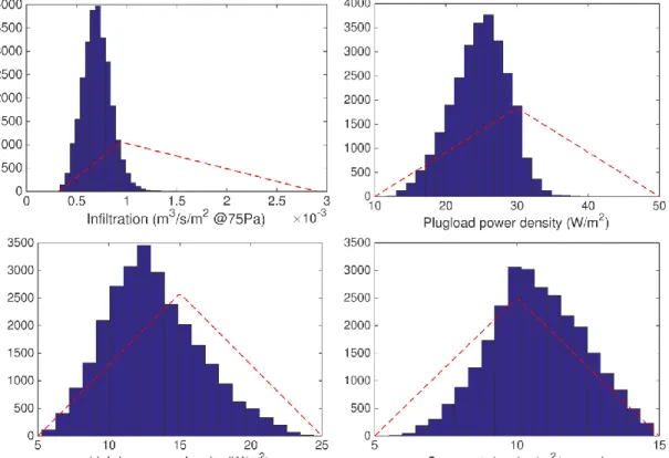
The four calibration parameters were calibrated using Bayesian calibration using monthly electricity and natural gas consumption. The prior probability density functions and calibrated PDFs are shown in Figure 2 by dashed lines
3025
, Page 5
and vertical bars respectively. It is clear from Figure 2 that the uncertainty distributions for both the infiltration rate and plugload power density BEM parameters calibrated well using Bayesian calibration, with both having significantly reduced uncertainty (variance) at the end of the calibration process. The lighting power density and occupant density parameters were less sensitive to calibration, with both the mean and variance of the prior and final PDFs being relatively constant for both parameters.
Figure 2: Prior (dashed line) and posterior (vertical bars) probability density functions for selected calibration parameters
The results of the calibration on the BEM projected electricity and natural gas consumption are given in Figure 3, which shows the monthly pre-calibrated and calibrated BEM output consumption against the monthly metered data. It is clear from Figure 3 that Bayesian calibration dramatically reduces the error between metered and BEM projected monthly electricity consumption. The calibration also reduced the error between metered and BEM projected monthly natural gas consumption, but moderate error still exists. This is primarily due to the fact that a nearly linear relationship exists between the plugload power density and lighting power density calibration parameters and the BEM projected electricity consumption.
3025
, Page 6
Figure 3: Pre-calibrated and calibrated building energy model projected monthly electricity (above) and natural gas (below) consumption relative to monthly metered consumption
6. CONCLUSION
Bayesian calibration is a method of calibration that is fundamentally different than conventional expert based, multivariate optimization, or machine learning calibration methods which overcomes a majority of the shortcomings of conventional calibration schemes. The primary advantage of Bayesian calibration is that it provides a most probable quantification of the uncertainty inherent in the calibration parameters and thus in the model outputs, allowing for probabilistic analysis, risk assessment, and confidence interval determination. This provides a greater level of information than conventional deterministic calibration procedures. Additionally, a model calibrated with Bayesian calibration yields the most probable uncertainty PDFs for the calibration parameters that is consistent with the observed data and prevents overfitting. This means that future model outputs from the calibrated model should have minimal error with respect to future observed data, given that the future combination of parameters for observed data are within the uncertainty bounds of the calibration parameters in the model. Parameter screening and efficient sampling methods help reduce the cost of data collection and computational demand of Bayesian calibration. A numerical example was included that highlights the application of Bayesian calibration to building energy modeling.
NOMENCLATURE
The nomenclature should be located at the end of the text using the following format:
BEM building energy model
DX direct expansion
EEM energy efficiency measure
LEED Leadership in Energy and Environmental Design
0 1000 2000 3000 4000 5000 6000 7000 8000 9000
Jan Feb Mar Apr May Jun Jul Aug Sep Oct Nov Dec
E le ct ri ci ty [ M J]
Meter Before Calibration After Calibration
0 2000 4000 6000 8000 10000 12000
Jan Feb Mar Apr May Jun Jul Aug Sep Oct Nov Dec
N at u ra l G as [ M J]
3025
, Page 7
NREL National Renewable Energy Laboratory PDF probability density function
REFERENCES
Bergerson, J., & Muehleisen, R. T. (2015). Bayesian Large Model Calibration Using Simulation and Measured Data for Improved Predictions. SAE Int. J. Passeng. Cars - Mech. Syst., 8(2). doi:10.4271/2015-01-0481
Campolongo, F., Cariboni, J., Saltelli, A., & Schoutens, W. (2005). Enhancing the Morris Method. Proceedings of the 4th International Conference on Sensitivity of Model Output, (pp. 369-379).
Cawley, G. C., & Talbot, N. L. (2010). On Over-Fitting in Model Selection and Subsequent Selection Bias in Performance Evaluation. J. Mach. Learn. Res., 11(August), 2079-2107.
Dietterich, T. (1995). Overfitting and Undercomputing in Machine Learning. ACM Comput. Surv., 27(3), 326-327. doi:10.1145/212094.212114
Dunsmore, I. R. (1968). A Bayesian Approach to Calibration. Journal of the Royal Statistical Society, Series B (Methodological), 30(2), 396-405.
Heckerman, D. (1998). A Tutorial on Learning with Bayesian Networks. In M. I. Jordan (Ed.), Learning in Graphical Models (Vol. NATO ASI Series 89, pp. 301-354). Netherlands: Springer. Retrieved from http://link.springer.com/chapter/10.1007/978-94-011-5014-9_11
Heo, Y., Augenbroe, G. A., & Choudhary, R. (2011). Risk Analysis of Energy-Efficiency Projects Based on Bayesian Calibration of Building Energy Model. Building Simulation 2011. Retrieved from http://www.ibpsa.org/proceedings/BS2011/P_1799.pdf
Kennedy, M. C., & O'Hagan, A. (2001). Bayesian Calibration of Computer Models. Journal of the Royal Statistical Society: Series B, 63(3), 425-464.
New, J., & Chandler, T. (2013). Evolutionary Tuning of Building Models to Monthly Electrical Consumption.
ASHRAE Transactions, 119(89).
Racine-Poon, A. (1988). A Bayesian Approach to Nonlinear Calibration Problems. Journal of the American Statistical Association, 83(403), 650-656. doi:10.2307/2289287
Raftery, P., Keane, M., & O'Donnell, J. (2011). Calibrating Whole Building Energy Models: An Evidence-Based Methodology. Energy and Buildings, 43(9), 2356-2364. doi:10.1016/j.enbuild.2011.05.020
Reddy, T., Maor, I., & Panjapornpon, C. (2007). Calibrating Detailed Building Energy Simulation Programs with Measured Data - Part I: General Methodology (RP-1051). HVAC&R Research, 13(2), 221-241.
Riddle, M., & Muehleisen, R. T. (2014). A Guide to Bayesian Calibration of Building Energy Models. Building Simulation Conference. Atlanta, GA: ASHRAE.
ACKNOWLEDGEMENT
The authors would like to acknowledge Yuming Sun for assistance in Bayesian calibration example used in this study and Brian Ball for providing the basic building energy model and measured data used for the example. This work was supported by the U. S. Department of Energy under Contract No. DE-AC02-06CH11357 with Argonne National Laboratory.