ANALYSIS AND OPTIMIZATION OF CLOSED-LOOP MANIPULATOR
CALIBRATION WITH FIXED ENDPOINT
Marco Antonio Meggiolaro
Pontifical Catholic University of Rio de Janeiro (PUC-Rio), Department of Mechanical Engineering Rua Marquês de São Vicente 225, Rio de Janeiro, RJ, Brazil 22453-900, [email protected] Guglielmo Scriffignano
Politecnico di Milano, Dipartimento di Meccanica, V. Bonardi, 9, 20133 Milano, Italy Steven Dubowsky
Massachusetts Institute of Technology, Department of Mechanical Engineering 77 Massachusetts Ave, Cambridge, MA 02139 USA
Abstract. This paper investigates a calibration method where the manipulator end-effector is
constrained to a single contact point using a fixture equivalent to a spherical joint. The required fixture has the advantage of being inexpensive and compact when compared to pose measuring devices required by other calibration techniques, such as theodolites. By forming the manipulator into a mobile closed kinematic chain, the kinematic loop closure equations are adequate to calibrate the manipulator as it executes self-motions, without the need of endpoint measurements or precision points. Adding a wrist force sensor allows for the calibration of elastic effects due to end-point forces and moments. A performance index is introduced to calculate the optimal location of the calibration device. The method is evaluated experimentally on a Schilling Titan II manipulator. The results show that the calibration method is able to effectively identify and correct for the errors in the system.
Keywords: manipulator, calibration, closed-loop, self-motions, optimization. 1. INTRODUCTION
Model based error compensation of a robotic manipulator, also known as robot calibration, is a process to improve manipulator position accuracy using software. Classical calibration involves identifying an accurate functional relationship between the joint transducer readings and the workspace position of the end-effector in terms of parameters called generalized errors (Roth et al., 1987). This relationship is found from measured data and used to predict, and compensate for, the endpoint errors as a function of configuration.
Considerable research has been performed to make manipulator calibration more effective both in terms of required number of measurements and computation by the procedure (Hollerbach, 1988; Hollerbach and Wampler, 1996; Roth et al., 1987). Several calibration techniques have been used to improve robot accuracy (Roth et al., 1987), including open and closed-loop methods (Everett and Lin, 1988). Open-loop methods require an external metrology system to measure the end-effector pose, such as theodolites. Obtaining open-loop measurements is generally very costly and time consuming, and must be performed regularly for very high precision systems. In contrast, closed-loop methods only need joint angle sensing, and the robot becomes self-calibrating. In closed-closed-loop calibration, constraints are imposed on the end-effector of the robot, and the kinematic loop closure equations are adequate to calibrate the manipulator from joint readings alone. Past closed-loop
methods have had the robot moving along an unsensed sliding joint at the endpoint, or constraining the end-effector to lie on a plane (Ikits and Hollerbach, 1997; Zhuang et al., 1999).
This paper investigates a closed-loop calibration method that was among a number suggested by (Bennett and Hollerbach, 1991). In the method, called here Single Endpoint Contact (SEC) calibration, the robot endpoint is constrained to a single contact point. Using an end-effector fixture equivalent to a ball joint, the robot executes self-motions to move to different configurations. At each configuration, manipulator joint sensors provide data that is used in an SEC identification algorithm to estimate the robot’s parameters. A total least squares optimization procedure is used to improve the calibration accuracy (Hollerbach and Wampler, 1996).
In addition to geometric errors, this calibration method is able to identify elastic structural deformation errors due to task loads and gravity, since arbitrary forces can be applied to the SEC fixture. The error model is extended to include the elastic errors, by explicitly considering the task loading and payload weight dependency of the errors. This is done by incorporating a method called GEC, which has been developed to identify the elastic errors as a function of the manipulator’s configuration and task loading wrenches at the end-effector (Meggiolaro et al., 1998).
Results presented here show that the location selected for endpoint contact significantly affects SEC calibration performance. A technique to find the optimal calibration point is presented with simulation results. The calibration method is applied experimentally to a 6 DOF hydraulic manipulator. The error parameters of the robot are identified and used to predict, and compensate for, the endpoint errors as a function of configuration. These experimental results show that the method is able to effectively and significantly improve the manipulator’s accuracy without requiring special and expensive metrology equipment.
2. ANALYTICAL BACKGROUND
The distortion of a manipulator from its ideal shape due to such factors as manufacturing errors results in the reference frames that define the manipulator joints being slightly displaced from their expected, ideal locations. This creates significant end-effector errors when the manipulator’s ideal model is used to predict its performance. The position and orientation of a manipulator’s frame Fireal with respect to its ideal location Fiideal is represented by a 4x4 homogeneous matrix Ei. The translational part of matrix Ei is composed of 3 coordinates, and the rotational part of matrix Ei is the result of the product of three consecutive rotations. These 6 parameters are called generalized error parameters, which can be a function of the system geometry and joint variables (Everett and Suryohadiprojo, 1988). For an n degree of freedom manipulator, there are 6(n+1) generalized errors. These can be represented in vector form as a 6(n+1) x 1 vector, called εεεε, assuming that both the manipulator and the location of its base are being calibrated. If only the manipulator is being calibrated, then the number of generalized errors is 6n.
The end-effector position and orientation error ∆∆∆∆X is defined as the 6x1 vector that represents the difference between the real position and orientation of the end-effector and the ideal one:
∆∆∆∆X = Xreal − Xideal (1)
where Xreal and Xideal are the 6x1 vectors composed of the three positions and three orientations of the end-effector reference frame in the inertial reference system for the real and ideal cases, respectively. Since the generalized errors are small, ∆∆∆∆X can be calculated using the linear equation in εεεε given by ∆∆∆∆X = Jeεεεε, where Je is the 6x6(n+1) Jacobian matrix of the end-effector error ∆∆∆∆X with respect to the elements of the generalized error vector εεεε, also known as Identification Jacobian matrix (Zhuang et al., 1999). If the generalized errors, εεεε, can be found from calibration measurements, then the correct end-effector position and orientation error can be calculated and compensated.
The identification of the 6(n+1) components of generalized errors εεεε for an n DOF manipulator is based on measuring the components of the end-effector error vector ∆∆∆∆X at a finite number (m) of different manipulator configurations. The m configurations are represented by m vectors of joint variables, q1, q2,…, qm. The equation ∆∆∆∆X = Jeεεεε can be written m times:
∆ ∆ ∆ ∆ X X X X J J J J 1 2 m t e 1 e 2 e m t q q q = = ⋅ = ⋅ ... ( ) ( ) ... ( ) εεεε εεεε (2)
where ∆∆∆∆Xt is the m x 1 vector formed by all measured vectors ∆∆∆∆X at the m different configurations
and Jt is the 6m x 6(n+1) Total Identification Jacobian matrix. To compensate for the effects of
measurement noise, the number of measurements m is in general much larger than n.
If the generalized errors are constant, then a unique least-squares estimate εεεε can be calculated by (Roth et al., 1987):
(
)
1
εεεε= J JtT − J ⋅∆∆∆∆X
t tT t (3)
If the Identification Jacobian matrix Je(qi) contains linear dependent columns, then Eq. (3) will
give estimates with poor accuracy. This occurs when there is redundancy in the error model, in which case it is not possible to distinguish the amount of the error contributed by each generalized error εij. To eliminate this problem, the columns of Je must be reduced to a linear independent set (Schröer, 1993). This reduction can be performed analytically by using the equations presented in (Meggiolaro and Dubowsky, 2000). The generalized errors are then grouped into a smaller independent set, resulting in identification with improved accuracy.
However, most manipulator calibration techniques to obtain the measurements in Eq. (2) require expensive and/or complicated pose measuring devices, such as theodolites. Thus the current interest in closed-loop methods that do not require such equipment. The SEC closed-loop calibration method, which uses data only from the internal sensors of a robot, is described below.
3. SINGLE ENDPOINT CONTACT (SEC) CALIBRATION
In Single Endpoint Contact calibration, instead of moving the end-effector to different positions to obtain the calibration measurements in Eq. (2), the endpoint position is kept fixed with changes only in its orientation. This is equivalent to grasping a ball joint, resulting in three calibration equations per pose. The advantage of this method is that it does not require measurements of the robot position using external sensors, requiring only an inexpensive and compact device such as a ball joint. Only one endpoint needs to be known and the joint angle measurements. The kinematic loop closure equations are enough to calibrate the manipulator from joint readings alone. In order to calibrate the system, the closed chain must have some mobility. So, a spatial manipulator must have 4 DOF's or more to be calibrated using this method. For planar manipulators, the point contact condition provides 2 constraints, so a robot with as few as 3 DOF's may be calibrated using SEC.
Consider the manipulator gripping the end-effector fixture at a constant location (x0,y0,z0), and define qreal as the measured vector of joint variables. The end-effector error is the difference between the actual position of the end-effector, at the SEC fixture, and the ideal position calculated from the ideal kinematic equations applied to the measured qreal. This ideal position is the end-effector position that an ideal manipulator would achieve if it was moved to the measured joint readings of the actual robot. As both ideal and real manipulator positions are evaluated at the same configuration qreal, the resulting end-effector error ∆∆∆∆X is only due to the generalized errors. From Eq. (1), the end-effector position error ∆∆∆∆X is
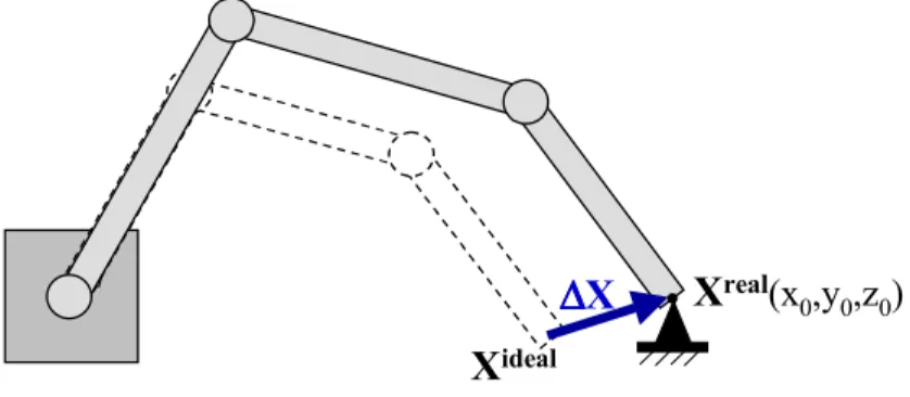
∆∆∆∆X = Xreal(qreal)−Xideal(qreal) = [x0,y0,z0]T−Xideal = Je(qreal) εεεε (4) Here the three end-effector reference frame orientations are eliminated from the error model, as they are not measured. The three position components of the end-effector reference frame in the inertial reference system are represented by the 3x1 endpoint vectors Xreal and Xideal, see Fig. (1). Since both Je and Xideal can be calculated at each point using the measured joint positions and ideal direct kinematics, the only remaining unknown in Eq. (4) is the generalized error vector εεεε.
∆∆∆∆X Xreal(x
0,y0,z0)
Xideal
Figure 1. Real and Ideal Positions of a Manipulator End-Effector
So, as the robot executes self-motions to different configurations, the real robot parameters can be estimated from the readings of the internal position sensors and from the identification model. A total least squares optimization procedure, shown in Eq. (3), is then used to improve the calibration accuracy.
As in every calibration not having a priori knowledge of the task constraint dimensions, the scale of the mechanism must be set, i.e., one link length or other length parameter has to be measured by independent means (Bennett and Hollerbach, 1991). In the SEC method, if any of the coordinates x0, y0 or z0 of the end-effector fixture is known, then this scaling requirement is already satisfied. However, if none of these coordinates is known, then one length parameter needs to be independently measured. Note that it is not necessary to know a priori the location of the end-effector fixture, since its location can be introduced as an unknown. In this case, Eq. (4) is rewritten
* * ε ε ideal J ε ε J X z y x 1 0 0 0 1 0 0 0 1 0 0 0 = ⋅ − − − = − (5)
where the unknown vector εεεε∗∗∗∗ contains both generalized errors and the coordinates of the end-effector fixture.
In addition to geometric errors, this calibration method is able to identify elastic structural deformation errors, since arbitrary forces can be applied to the SEC fixture. In this case, an extended error model must be used to identify the elastic errors as a function of the payload wrench at the end-effector, as discussed before. Defining F as the desired force applied to the end-effector and J as the robot Jacobian, then the vector ττττ of applied joint torques/forces to the manipulator would be ττττ = JT (−−−−F).
4. OPTIMIZATION OF THE FIXTURE LOCATION
In SEC calibration, the location of the endpoint device can significantly affect the calibration performance. Ideally, the generalized errors are constant in their frames, and the errors identified at an arbitrary configuration can be used to compensate the errors at any other configuration. In this
case, the chosen location used by the SEC does not influence the calibration accuracy, since any configuration would lead to the same constant generalized errors. However, the generalized errors are in general functions of the configuration, especially in systems with significant elastic deformation. Therefore, interpolating functions must be chosen to model each generalized error, and its coefficients must be identified (Meggiolaro et al., 1998).
Furthermore, depending on the chosen set of measurement points, the error compensation process involves interpolation or extrapolation of the generalized error functions. As a general mathematical result, the interpolation accuracy can be improved to the limit of the measurement noise by performing enough measurements in the desired range. But the extrapolation accuracy depends on the chosen set of functions, especially on how well they model the actual system. So, poorly chosen functions may give a reasonable precision in the interpolation range, but its accuracy is compromised in configurations outside the measured range. As a result, the choice of the measurement ranges at each joint is critical to the calibration accuracy.
In the SEC calibration, the measurement ranges of each joint are uniquely defined by the location of the calibration point. For a generic manipulator, it is necessary to use numerical methods to find the measurement ranges (Burdick, 1989; Meggiolaro et al., 2000). If the manipulator inverse kinematic equations can be written, then it is possible to find analytical solutions for the joint ranges. For an ideal 3R planar manipulator, with full-range of all 3 joints and no interference between links, an analytical solution of the measurement ranges for each calibration point P has been found, as given below.
Defining li as the length of link i and P = [r cos ϕ, r sin ϕ] as the calibration point, the joint angles qi must satisfy:
12 1 2 3 2 2 1 2 1 1 2 3 2 2 1 2 11 k r l 2 ) l (l l r ) cos(q r l 2 ) l (l l r k ≡ + − + ≤ −ϕ ≤ + − − ≡ 22 2 1 2 2 2 1 2 3 2 2 1 2 2 2 1 2 3 21 2l l k l l ) l (r ) cos(q l l 2 l l ) l (r k ≡ − − − ≤ ≤ + − − ≡ 32 3 2 2 3 2 2 2 1 3 3 2 2 3 2 2 2 1 31 k l l 2 l l ) l (r ) cos(q l l 2 l l ) l (r k ≡ − − − ≤ ≤ + − − ≡ (6)
The calibrated range of a joint j can then be written as: ] q q , q [q ] q q , q [q qj∈ j0− j1 j0− j2 ∪ j0+ j2 j0+ j1 (7) where 1 k 1 1 k 1 k if if if ) acos(k 0 π q ji ji ji ji ji ≤ ≤ − ≥ − ≤ ≡ and 3 j if 0 2 j if 0 1 j if qj0 = = = ϕ ≡ (8)
For a generic 3R manipulator, it is also necessary to consider the intersection between the ideal solution from Eqs. (7-8) and the mechanical limits of each joint.
Once the measurement ranges of each joint are calculated and the errors identified using SEC, the calibration performance can be evaluated by defining a performance index. This index is based on the idea that measurement interpolation results in better accuracy than extrapolation. First consider the Interpolated Compensation Region (ICR), defined as the region of the workspace where the compensation algorithm does not require extrapolation of the error functions. It represents the region of the workspace that the manipulator can reach by independently sweeping its joints through their interpolated ranges. Conversely, the Extrapolated Compensation Region (ECR)
is the workspace region where any of the generalized error functions needs to be extrapolated, resulting in reduced accuracy.
In order to obtain an ideal location of the calibration point, a performance index for the SEC method needs to be defined and optimized. The volume of the ICR is an example of such index. As a calibration point P is chosen to maximize this volume - therefore minimizing the volume of the ECR - the overall accuracy of the compensation algorithm is increased. But in this way, every region of the workspace is given the same importance, even those that are not useful for the task to be performed after calibration. To choose the fixture location that offers the best accuracy in specific workspace regions, a more general index is defined, called the Weighted Volume of the ICR (WV):
∫∫∫
α ⋅= ICR (x,y,z) dV
WV (9)
where α(x,y,z)∈[0,1] is a weight function defined in the whole workspace, representing the importance of each point (x,y,z) on the chosen task. Note that if α(x,y,z)=1 in the whole workspace, then the WV becomes the geometric volume of the ICR. The choice of the best fixture location for the SEC method is obtained by maximizing the function WV.
5. RESULTS
Simulations of the SEC calibration and the optimization of the fixture location were performed for two 3R planar manipulators and a 6-DOF manipulator. Experiments were then performed on a Schilling Titan II manipulator to show the effectiveness of the SEC calibration.
5.1. Simulation Results
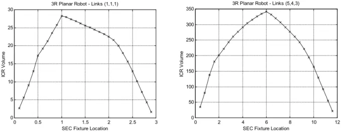
Two different 3R planar manipulators were considered, with link lengths (1, 1, 1) and (5, 4, 3). In both cases an optimal location of the SEC fixture was found. For the (1, 1, 1) manipulator, the location that maximizes the volume of the interpolated region is at a distance from the robot base equal to 1.0, see Fig. (2). By using this fixture location, it is possible to move the manipulator in the full-range of its 3 joints, and the errors along the entire workspace can be compensated without extrapolation. Note that in this example the considered weights α(x,y,z) of the Weighted Volume are equal to 1.0, i.e., every region of the workspace is considered equally important.
0 0.5 1 1.5 2 2.5 3 0 5 10 15 20 25
30 3R Planar Robot - Links (1,1,1)
ICR V
ol
um
e
SEC Fixture Location
0 2 4 6 8 10 12 0 50 100 150 200 250 300
350 3R Planar Robot - Links (5,4,3)
SEC Fixture Location
IC R V ol um e
Figure 2. ICR Volume as a Function of the Fixture Location for Link Lengths (1, 1, 1) and (5, 4, 3) For the (5, 4, 3) planar manipulator, the optimal solution of the fixture location is at a distance from the robot base equal to 6.0 (see Fig. (3), left figure). In this case, however, the ICR is not
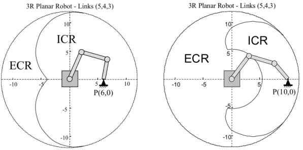
coincident with the workspace. The maximum volume (or area, since it's a planar manipulator) of the ICR is 341.6, while the workspace surface is π⋅122 = 452.4. So, even for the best choice of the calibration point, still 25% of the calibrated workspace relies on extrapolation to compensate for the measured errors. Figure (3) (left) shows some of the 3R manipulator configurations corresponding to a fixture location at P(x,y)=(6,0). The Interpolated and Extrapolated Compensation Regions obtained after the calibration process at two different fixture locations are shown in Fig. (3). Note that the ICR obtained from calibration at the optimal fixture location P=(6,0) is much larger than the one obtained using P=(10,0). Thus it is expected that the SEC calibration at P=(6,0) results in better accuracy than using a fixture location at P=(10,0).
3R Planar Robot - Links (5,4,3)
-10 -5 0 5 10 5 10 -10 -5 P(6,0)
ICR
ECR
3R Planar Robot - Links (5,4,3)
-10 -5 0 5 -10 5 10 -5 P(10,0)
ICR
ECR
Figure 3. Extrapolated and Interpolated Compensation Regions for an SEC Fixture at (6,0) or (10,0) A simulation of the SEC method was applied to a 3R planar manipulator with link lengths (1m, 1m, 1m). The simulation introduced generalized errors that are not constant in their reference frames, reflecting the effects of elastic deformations. To investigate the effects of interpolation and extrapolation on the measured errors, the chosen identification functions were different from the introduced error functions, otherwise the simulation would always result in a perfect fit.
Two different fixture locations are used in the calibration, at distances 1.0m (the optimal location in this case) and 2.5m from the manipulator base. The manipulator is moved to several measurement configurations, sweeping the joint ranges allowed by each fixture location. An RMS uncorrected error of 8.0mm and a measurement noise of 0.1mm were introduced to both simulations. After the identification process, the end-effector was released and the compensated manipulator was moved to all possible configurations in the workspace. The residual error after compensation was then evaluated at each configuration, and its RMS value was calculated.
For the calibration fixture at 1.0m, the full range of the three joints was achieved, and the RMS residual error was 0.16mm. When the fixture location was changed to 2.5m from the robot base, the RMS residual error was 0.49mm, approximately 3 times higher. This poorer accuracy is mainly due to the measurement range of joint 1 being restricted to the interval [−49o, 49o], therefore all configurations outside this range are compensated using extrapolations. Unless the chosen interpolation functions perfectly model the generalized errors, the SEC fixture location plays a critical role on the calibration accuracy.
Note that calibration cannot be made infinitely accurate as the number of measurement points is increased, and a lower bound exists on the calibration error that is dictated by robot repeatability and calibration measurement error (Roth et al., 1987). This lower bound can be achieved using a minimum number of measurement points, which depends on the measurement noise level. In this example, about 100 measurement points are necessary if the noise level is 0.1mm, 200 points for 0.5mm, and 300 if the noise is 1.0mm.
Simulations were also performed for a Schilling Titan II manipulator, a 6-DOF hydraulic robot. Using these results the SEC performance was analyzed for two different calibration device lengths: 10 and 50 inches (254 and 1270mm). These lengths are the distance between the device gripper, attached to the robot end-effector, and the center of rotation of the spherical joint. The device length plays an important role on the achievable measurement ranges, since it modifies the loop closure equations.
Due to the rotational symmetry of the system around joint 1, the optimal location of the calibration device is on the vertical plane defined by the middle of the mechanical limits of joint 1. The optimal location for the 254mm device is calculated at P(x, z) = (550mm, 1800mm), respectively the horizontal and vertical distances from the manipulator base along the defined vertical plane. The volume of the ICR in this case is 8.33m3. A second maxima for the ICR volume is 6.66m3, obtained for a device location at P(x, z) = (550mm, -200mm) from the manipulator base. For the 1270mm device, the optimized location is at P(x, z) = (1600mm ,1750mm), resulting in an ICR volume of 17.8m3. Note that this volume is twice the ICR volume obtained from the 254mm device, i.e., the 1270mm fixture results in a better calibration accuracy in this case.
5.2. Experimental Results
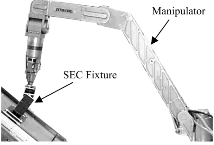
Figure (4) shows the laboratory system used to experimentally evaluate the SEC calibration method. The manipulator is a Schilling Titan II, a six DOF hydraulic robot capable of handling payloads in excess of 100 kg. A handle on the SEC fixture provides a repeatable grip for the manipulator.
Figure 4. Experimental System
The objective of the experiment is to see if the SEC calibration method can be practically applied to a real physical system to improve its absolute accuracy. The object is to have the residual error approach the limit set by the position sensing resolution of the system. A control technique called Base Sensor Control (Iagnemma et al., 1997) is used to improve the system repeatability by greatly reducing the effects of joint friction. The relative positioning root mean square error is used as a measure of the system repeatability. Data is taken by moving the manipulator an arbitrary distance from the test point and then commanding it back to its original position. The measured maximum errors are ±5 mm, and the repeatability of the system is 2.7 mm (RMS).
Although the Base Sensor Control algorithm greatly reduces the repeatability errors, there are still 45mm (RMS) errors in absolute accuracy. Since the system repeatability is relatively small with respect to the absolute errors, a model based error compensation method can be applied to reduce the accuracy errors, such as the SEC method.
In order to implement SEC, the generalized error functions were interpolated using approximately 800 measurements of the robot configuration. These measurements were performed for an SEC device with length 155mm located at P(x, z) = (1440mm, 265mm) from the manipulator
Manipulator
base. Note that the end-effector fixture location was obtained by the SEC calibration, since it was not known a priori. After the identification process, the compensated manipulator was moved to 200 different configurations to verify the efficiency of the SEC method.
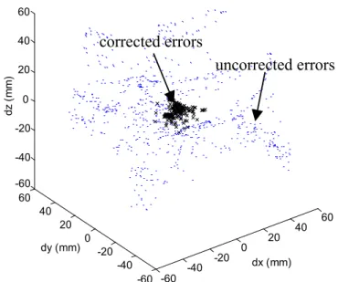
Figure (5) shows the convergence of original positioning errors as large as 98.5mm (44.8mm RMS) to corrected absolute errors of less than 15mm (5.7mm RMS) with respect to the base frame. This demonstrates an overall factor of nearly 8 improvement in absolute accuracy by using the SEC calibration algorithm. This improvement in performance shows that such calibration method is able to effectively identify and correct for the errors in the system.
-60 -40 -20 0 20 40 60 -60 -40 -20 0 20 40 60 -60 -40 -20 0 20 40 60 dx (mm) dy (mm) dz ( m m )
Figure 5. Measured and Residual Errors After Compensation 6. CONCLUSIONS
In this paper, a calibration method that does not require endpoint measurements or precision points has been investigated. The method constrains the robot end-effector to a fixture equivalent to a spherical joint. The required fixture has the advantage of being inexpensive and compact when compared to pose measuring devices required by other calibration techniques. By forming the manipulator into a mobile closed kinematic chain, the kinematic loop closure equations are adequate to calibrate the manipulator from joint readings alone. A performance index is introduced to calculate the optimal location of the calibration device. The method is evaluated experimentally on a Schilling Titan II manipulator. The results show that the calibration method is able to effectively identify and correct for the errors in the system.
7. ACKNOWLEDGMENTS
The support of the Korean Electric Power Research Institute (KEPRI), Electricité de France (EDF), and the Brazilian government (through CAPES) in this research is appreciated.
8. REFERENCES
Bennett, D.J. and Hollerbach, J.M., 1991, "Autonomous Calibration of Single-Loop Closed Kinematic Chains Formed by Manipulators with Passive Endpoint Constraints", IEEE Trans. Robotics & Automation, Vol. 7, No. 5, pp.597-606.
Burdick, J.W., 1989, “On the Inverse Kinematics of Redundant Manipulators: Characterization of the Self-Motion Manifolds”, Proceedings of the IEEE International Conference on Robotics and Automation, Vol. 1, pp. 264-270.
uncorrected errors corrected errors
Everett, L.J., Lin, C.Y., 1988, “Kinematic Calibration of Manipulators with Closed Loop Actuated Joints,” Proc. IEEE International Conf. On Robotics and Automation, Philadelphia, pp.792-797. Everett, L.J., Suryohadiprojo, A.H., 1988, “A Study of Kinematic Models for Forward Calibration
of Manipulators,” Proc. IEEE Int. Conf. Robotics and Automation, Philadelphia, pp.798-800. Hollerbach, J., 1988, “A Survey of Kinematic Calibration,” Robotics Review, Khatib et al ed.,
Cambridge, MA, MIT Press.
Hollerbach, J.M., Wampler, C.W., 1996, “The Calibration Index and Taxonomy for Robot Kinematic Calibration Methods,” Int. J. of Robotics Research, Vol. 15, No. 6, pp.573-591. Iagnemma, K., Morel, G. and Dubowsky, S., 1997, “A Model-Free Fine Position Control System
Using the Base-Sensor: With Application to a Hydraulic Manipulator,” Symposium on Robot Control, SYROCO ‘97, Vol. 2, pp. 359-365.
Ikits, M., Hollerbach, J.M., 1997, “Kinematic Calibration Using a Plane Constraint,” IEEE International Conference on Robotics and Automation, pp. 3191-3196.
Meggiolaro, M., Mavroidis, C. and Dubowsky, S., 1998, “Identification and Compensation of Geometric and Elastic Errors in Large Manipulators: Application to a High Accuracy Medical Robot,” Proceedings of the 1998 ASME Design Engineering Technical Conference, Atlanta. Meggiolaro, M. and Dubowsky, S., 2000, “An Analytical Method to Eliminate the Redundant
Parameters in Robot Calibration,” Proc. of IEEE Int. Conference on Robotics and Automation (ICRA 2000), pp. 3609-3615, Stanford, CA
Meggiolaro, M., Scriffignano, G., Dubowsky, S., “Manipulator Calibration Using a Single Endpoint Contact Constraint", 26th Biennial Mechanisms Conference, Baltimore, Maryland, DETC2000/MECH-14129, ASME, 2000.
Roth, Z.S., Mooring, B.W., Ravani, B., 1987, “An Overview of Robot Calibration,” IEEE Journal of Robotics and Automation, Vol. 3, No. 5, pp.377-384.
Schröer, K., 1993, Theory of Kinematic Modeling and Numerical Procedures for Robot Calibration. In Bernhardt, R., Albright, S.L. eds.: Robot Calibration. London: Chapman & Hall, pp.157-196. Yang, D.C.H. and Lee, T.W., 1983, “On the Workspace of Mechanical Manipulators”, Transactions
of the ASME, Journal of Mechanical Design, Vol. 105, pp. 62-69.
Zhuang, H., Motaghedi, S.H., Roth, Z.S., 1999, “Robot Calibration with Planar Constraints,” Proc. IEEE International Conference of Robotics and Automation, Detroit, Michigan, pp.805-810.