Earnings Yield and Predictability in the Dry Bulk Shipping Industry

City, University of London Institutional Repository

Citation

:

This is the accepted version of the paper.

This version of the publication may differ from the final published

version.

Permanent repository link:

Link to published version

:

Copyright and reuse:

City Research Online aims to make research

outputs of City, University of London available to a wider audience.

Copyright and Moral Rights remain with the author(s) and/or copyright

holders. URLs from City Research Online may be freely distributed and

linked to.

City Research Online: http://openaccess.city.ac.uk/ publications@city.ac.uk

City Research Online

Shipping Industry

IOANNIS C. MOUTZOURIS

_{AND NIKOS K. NOMIKOS}

a _{Cass Business School, Faculty of Finance, City, University of London, 106 Bunhill Row, London EC1Y 8TZ, UK.}

Email: Ioannis.Moutzouris@city.ac.uk.

b _{Corresponding author: Cass Business School, Faculty of Finance, City, University of London, 106 Bunhill Row,}

London EC1Y 8TZ, UK. Contact number: +44 (0)20 7040 0104. Email: N.Nomikos@city.ac.uk.

Abstract

We examine the relation between vessel prices, net earnings and holding period returns in the dry bulk shipping industry. In doing so, we provide a framework for pricing shipping assets, with finite economic lives and also subject to wear and tear. Shipping earnings yields negatively forecast future net earnings growth while there is no consistent evidence of time-varying risk premia. We provide an economic interpretation for the obtained results and argue that the investment decisions of shipowners affect the current price of the asset through the expected cash flow stream, thus implying cash flow predictability.

Keywords: Valuation of Transportation Assets; Shipping Cash Flow Predictability; Shipping Risk Premia; Variance Decomposition of Earnings.

JEL Codes: C13, G12, R40.

I.

Introduction

This article examines the relation between vessel prices, net earnings, and holding-period returns in the dry bulk shipping industry. The motivation for this study stems from the fact that expected returns and changes in net earnings form the rational benchmarks for the interpretation of variation in assets’ valuation ratios (Bansal and Yaron, 2004). There is plentiful evidence on the predictability of those variables from the equity and real estate markets. For instance, it has been shown that in the larger equity markets, such as those of US, UK, and Germany, virtually all variation in dividend yields is the result of time-varying expected future returns or, equivalently, time-varying risk premia (Ang and Bekaert, 2007). Namely, dividend yields positively forecast future returns while dividend growth appears to be unpredictable (Cochrane, 2005). Consequently, the bulk of empirical asset pricing research has concentrated on time-varying discount-rate theories to explain the formation of asset prices (Cochrane, 2011). On the other hand, Ghysels et al (2012) illustrate that the bulk of rent yield volatility in the U.S. real estate sector can be attributed to variation in future rent growth as opposed to variation in future returns.

To examine the question of relative predictability in dry-bulk shipping, we extend the Campbell-Shiller variance decomposition and vector autoregression (VAR) frameworks (1988a and 1988b) to the case of real assets with limited economic lives. We illustrate, for the first time in the literature, that vessel prices appear to move mainly due to news about future shipping market conditions and not due to changes in the risk premia required by shipping investors. In addition,we provide an economic interpretation for the obtained results and a comparison to different industries.

Regarding the existing shipping literature, Kavussanos and Alizadeh (2002) identify a long-run cointegrating relationship between net earnings and vessel prices and apply the Campbell and Shiller (1988a) VAR framework to test the validity of the Efficient Market Hypothesis in the formation of dry bulk vessel prices. Alizadeh and Nomikos (2007) suggest that shipping earnings yields contain useful information about future market conditions that can benefit agents’ investment decisions. Greenwood and Hanson (2015) suggest, but do not justify empirically, that the earnings yield must strongly forecast low future earnings growth. Papapostolou et al (2014) use the earnings yield as a market valuation proxy to construct a shipping sentiment index and, in turn, argue that a high earnings-yield ratio serves as a contrarian indicator for future shipping conditions. The latter argument is in line with Greenwood and Hanson (2015) but also with Papapostolou et al (2017) who use the PE ratio (that is the inverse of the earnings yield) as a valuation-specific metric to examine herd behaviour in the decision to invest in new or retire existing fleet capacity in the dry bulk shipping industry. Nevertheless, none of those papers examine formally the relation between shipping earnings yields and future net earnings growth.

Alizadeh et al (2017) incorporate a heterogeneous-agents model (HAM) and argue that heterogeneity in beliefs and investment behaviour by market participants can explain the price volatility of dry bulk second-hand vessels. While our motivation is similar, our model examines the behaviour of earnings yield (and in turn, vessel prices) incorporating the traditional view of asset pricing (along the lines of Campbell and Shiller, 1988a and b and Cochrane, 2005) according to which, asset prices are determined by either expectations about future cash flow growth and/or expectations about time-varying risk premia. Importantly, we illustrate that the representative market participant values second-hand vessels based on news about expected market conditions. To the best of our knowledge, we are the first to address formally this question in the shipping literature.

Extending the Campbell-Shiller asset pricing framework to shipping markets is of interest since, in contrast to equities, vessels are tangible assets with limited economic lives and thus, subject to economic depreciation. In analogy to the dividend and rent yields, the appropriate valuation ratio in shipping is the earnings yield, defined as the ratio of one-period net earnings to the current price of the respective second-hand vessel. Since shipping investors know in advance the net earnings they expect to receive for the forthcoming period, we construct a “forward-looking” earnings yield which is consistent with reality and market practice. Therefore, from a technical perspective, we extend the Campbell-Shiller variance decomposition and VAR frameworks (1988a and 1988b) to account for both “forward-looking” valuation ratios and economic depreciation in the value of the asset. To the best of our knowledge, this is the first time that these features are explicitly incorporated in this asset pricing framework. The proposed framework can also be easily extended to the valuation of assets in other real asset economies such as real estate or the airline industry; e.g. in real estate, owners also agree in advance with lessees upon the rent corresponding to the next period.

Shipping also provides an ideal environment to relate the Campbell-Shiller reduced-form estimation framework to the economic principles of the market as this is a capital-intensive industry with clear and directly observable supply and demand determinants. We argue that the major determinants of valuation ratios are the second-order effects that current cash flows have on current prices through the future (expected) cash flow stream. In the absence of second-order effects, there is no reason for future cash flows to be predictable by the current information filtration.

We illustrate that high earnings yields strongly and negatively predict future net earnings growth. Furthermore, there is no consistent evidence of time-varying expected returns in the second-hand dry bulk shipping industry. Equivalently, it seems that ship prices mainly vary due to news about expected market conditions per se and not due to time-varying risk premia; that is, when valuing vessels, shipowners appear not to require time-varying risk premia. Furthermore, since valuation ratios are indicators of the fundamental value of the asset relative to the generated cash flow, we argue that

vessels are undervalued – relatively to prevailing net earnings – when freight markets are very strong and vice versa.1

While the main aim of our paper is to provide a mathematically rigorous asset-pricing framework applicable for ships, our results also have practical implications for market practitioners. We show that the earnings yield is a reliable indicator of the current state of the shipping industry as well as of future shipping market conditions: a high earnings yield today reflects current prosperous market conditions but also predicts a deterioration in future net earnings and thus future market conditions. Therefore, the earnings yield can be used both as a forecasting variable and an indicator in trading strategies related to shipping assets. Another potential practical application of our research is related to shipping finance. Namely, the earnings yield can be used by providers of shipping finance when evaluating the business risk of their investment. Since the earnings yield predicts future market conditions, the higher the earnings yield at the issuance of the loan, the riskier the loan becomes ‒ ceteris paribus ‒ and thus, the higher the interest rate that should be demanded by lenders.

Finally, we compare our findings with those from the equity and real estate markets and explain the observed similarities and differences. Specifically, our results are diametrically opposite to the ones in the US, UK, and German equity markets but in line with the ones obtained from the bulk of international equity and real estate markets. It appears that the degree of cash flow predictability by the valuation ratio depends on the magnitude of second-order effects of current cash flows on future cash flows. Since, current prices depend on the expected cash flows generated by the asset, the more intensive those second-order effects are, the more predictable future cash flows become and, in turn, the more informative prices and valuation ratios become about future market conditions. Therefore, this paper provides strong evidence for further discussion regarding the economic principles that drive the forecasting properties of valuation ratios.

The remainder of this paper is organised as follows. Section II introduces the dataset employed and analyses the main variables of interest along with some preliminary results. Section III illustrates the methodology and the main empirical findings. Section IV provides both an economic rationale behind our results and a theoretical comparison with the equity and real estate markets. Section V concludes.

II.

Data and Variables of Interest

The dataset consists of monthly and quarterly observations on newbuilding (NB), second-hand (SH), and scrap vessel prices and 6-month and 1-year time-charter (TC) rates for the Capesize, Panamax,

1 _{The term over/under-valuation in our context describes the relationship between the vessel’s (asset’s) market}

value and the concurrent net earnings (cash flows) generated by the asset. Thus, it is different than the interpretation given under the Efficient Market Hypothesis that an asset is overvalued when its market price is above its fair fundamental value, or vice-versa. We thank an anonymous referee for suggesting that.

Handymax, and Handysize dry bulk sectors where, for each one, we have employed the largest available sample. In addition, we have obtained data for various supply and demand variables related to the dry bulk shipping industry. Our main shipping data source is Clarksons Shipping Intelligence Network 2010. Figures for operating and maintenance expenses for representative vessels in each sector, as of December 2014, are obtained through discussions with industry participants and our values agree with figures reported in the recent literature. These are also used as the base real value since these costs generally increase with inflation; data for the US Consumer Price Index (CPI) are obtained from Thomson Reuters Datastream Professional. Table 1 presents the sample characteristics for each dry bulk sector.

Table 1: Sample and sector characteristics for dry bulk shipping.

Sector Sample period 𝑇 Representative vessel (dwt) _{($/𝑑𝑎𝑦)}Costs Capesize 1/1992-12/2014 276 180,000 8,000

Panamax 1/1976-12/2011 432 76,000 7,000

Handymax 4/1986-6/2014 339 56,000 6,500

Handysize 1/1976-12/2014 468 32,000 5,500

Notes: The number of observations in the sample is denoted by 𝑇. Costs, expressed in December 2014 dollars per day, refer to the total operating and maintenance expenses of the vessel.

We use the price of the second-hand 5-year old vessel as the variable of interest. 2 _{We assume that} vessels are leased (chartered) in consecutive 1-year TC contracts; hence, only operating and maintenance costs are borne by the shipowner. In addition, we assume that vessels spend 10 days per annum off-hire for maintenance and repairs. During this period, shipowners do not receive the corresponding TC rates but bear the operating and maintenance costs (Stopford, 2009). We also consider the commission that the shipbroker receives for bringing the shipowner and the charterer into an agreement which is 2.5% of the daily TC rate. Thus, the annual net earnings variable, 𝛱+,-, is

calculated as:

𝛱_+,-≡ 𝛱_+→+,- = 355 ∙ 0.975 ∙ 𝑇𝐶_+→+,-− 365 ∙ 𝑂𝑃𝐸𝑋_+→+,-, (1)

2 _{We use second-hand values since, due to the construction lag between the ordering and delivery of a new}

vessel, newbuilding prices reflect the price of a vessel for future delivery and hence, are not directly connected to the prevailing rates in the market. Our second-hand price dataset consists of observations for 5, 10, 15, and 20-year old vessels. We have chosen the price of a 5-year old vessel as this is the most liquid segment of the second-hand market. Our results, however, are not sensitive to this choice. In addition, reports for vessel prices and TC rates do not refer to vessels of the same cargo-carrying capacity over the sample period. To overcome this limitation, we have constructed an earnings series by adjusting the original earnings rates to the size of the vessel, as in Greenwood and Hanson (2015). Due to a change in the reported time-charter rates for the Panamax Bulk-carrier in the database, the sample period ends in December 2011. For robustness, we also examined a shorter subsample, referring to a 75,000-dwt vessel, which spans March 2001 to December 2014, and the obtained results are similar with the ones reported here.

where 𝑇𝐶+→+,- and 𝑂𝑃𝐸𝑋+→+,- refer to the corresponding daily TC rates and the summation of daily

operating and maintenance expenses, respectively. Note that a feature of the shipping industry is that the shipowner knows his net earnings for the forthcoming period in advance: shipowners and charterers agree upon the TC rate of the vessel at the commencement of the corresponding period3 while this is also the case for the respective operating and maintenance expenses.

Since vessels are real assets with finite economic lives we must account for economic depreciation. Namely, at each point in time a 6-year old vessel is less valuable than an identical 5-year one because the former has one less year of future economic life, but also lower performance compared to the latter.4 _{Assuming that vessels are scrapped at the end of the 25}th _{year of their economic life, we denote} the price of a (5 + 𝑛)-year old vessel at time 𝑡 by 𝑃D,E,+, for 0 ≤ 𝑛 ≤ 20. As estimated in Appendix A,

ship prices are subject to 5% annual value depreciation and thus, the prices of vessels between 5 and 10 years of age can be estimated through:

𝑃_D,E,+= (1 − 0.05𝑛) ∙ 𝑃_D,+, 1 ≤ 𝑛 ≤ 5. (2) Accordingly, the 1-year horizon raw return is estimated as:

𝑅E,+→+,-≡ 𝑅E,+,-=

𝛱+,-+ 𝑃

E,-,+,-𝑃_E,+ , (3)

where 𝑅E,+,- is the holding-period real return realised at time 𝑡 + 1 from an investment made at time

𝑡 for a 𝑛-year old vessel. Intuitively, this formula assumes that an investor at time 𝑡 purchases the vessel at price 𝑃E,+ and immediately leases her out for one year to earn the 1-period net earnings,

𝛱_+,-. In turn, at 𝑡 + 1 the investor sells the vessel at the prevailing market price, 𝑃_E,-,+,-.5 Henceforth, we drop the age index from the notation for expositional simplicity.

In the context of empirical asset pricing, we examine the source of variation in vessel prices and in particular whether vessel prices vary due to changing forecasts about future net earnings, changes in future returns or variations in the terminal (scrap) price of the vessel. The main variable of interest in our empirical estimation is the shipping earnings yield, defined as the ratio of net earnings over the

3_{This assumption is consistent with both the existing shipping literature (e.g. Greenwood and Hanson, 2015) and}

market practice. In practice, ship owners and charterers agree upon the time-charter rate of the vessel – for the entire leasing period – before the corresponding leasing period begins. Accordingly, the agreed rates are typically received every 15 days - sometimes also in advance - which reduces the probability of default by the charterer. In addition, a wide broking network and the fact that ship owners normally lease their vessels to solvent charterers also assure transparency and low probability of default. Finally, additional contractual agreements included in the charter party ensure that the owner will receive the full time-charter rate agreed.

4 _{The implicit assumption that net earnings do not depend on the vessel’s age does not have a qualitative impact}

on the results. As such, we ignore the fact that vessels command a lower rate as their age increases.

5 _{When a vessel is sold in the second-hand market, transaction costs (the commission to the sale-and-purchase}

broker) amount to 1% of the resale price. In the context of this research, we ignore this transaction cost since it has no effect on the empirical results.

corresponding 5-year old vessel price, IJKL

MN,J, which measures the profit from utilising the vessel for the

period 𝑡 → 𝑡 + 1 as a fraction of the prevailing price of the asset at 𝑡. From an investor’s perspective, a high (low) earnings yield reflects the relative degree of undervaluation (overvaluation) in the price of the vessel.

While the shipping earnings yield is the natural analogue in shipping of the dividend and rent yields in equity and real estate markets, respectively, there is a significant difference in the definition of our shipping valuation ratio compared to the ones in the existing asset pricing literature. Specifically, in equity (real estate) markets, dividends (rents) corresponding to period 𝑡 → 𝑡 + 1 are assumed to be unknown at time 𝑡. Thus, the ratio OJ

MJ corresponds to the net income paid during period 𝑡 − 1 → 𝑡

divided by the asset price at 𝑡, where the price is net of the respective cash flow value. Campbell and Shiller (1988b) argue that dividends are lagged to be ℱ+-measurable. Hence, the buyer of the asset at

time 𝑡 is entitled to the net income stream {𝐷+,S}SU-. Earlier studies in the shipping literature

(Kavussanos and Alizadeh, 2002; Alizadeh and Nomikos, 2007) have also used an equivalent “lagged” definition of the earnings yield which in our notation corresponds to IJ

M_N,J.

However, in line with Papapostolou et al (2014), we suggest that the appropriate valuation ratio in shipping is “forward-looking” since net earnings corresponding to period 𝑡→ 𝑡 + 1, 𝛱+,-, are agreed

at time 𝑡 and thus, known in advance.6 _{Thus, the shipping cash flow not only serves as a forecasting} scheme for future cash flows but is also the first term of the expected generated cash flow series.7 While this should also be the case for real estate, the related existing literature ignores that feature (e.g. Campbell et al, 2009; Ghysels et al, 2012).

Table 2 presents descriptive statistics related to annual net earnings, 5-year old vessel prices, and earnings yields for the four dry bulk sectors while Figure 1 illustrates their evolution. As Figure 1 depicts, all three variables are very volatile. Autocorrelation coefficients in Table 2 are highly persistent in the 1-month horizon but decrease rapidly as the horizon increases, consistent with the

6 _{Namely, the owner of the vessel at time 𝑡 is entitled to the value of net earnings 𝛱}

+,-. Thus, assuming no credit

risk (as analysed in footnote 2) or other unforeseen risks and expenses (e.g. due to breakdowns, accidents, etc.), earnings are ℱ+-measurable.

7 _{In support of this statement, Fama and French (1988) argue that the most commonly incorporated dividend}

yield in equity markets, 𝐷+⁄ ,𝑃+ has the following drawback. While stock prices, 𝑃+, are forward-looking, the

incorporated dividend, 𝐷+, is “old” relative to the dividend expectations embedded in 𝑃+. Accordingly, positive

news about future dividends results in a high price relative to the last paid dividendwhich, in turn, implies a low current dividend yield. In turn, this increase in 𝑃+ produces a high return 𝑟+X-→+ and, as a result, there is negative

correlation between the disturbance 𝜀+X- and the time 𝑡 shock to 𝐷+⁄𝑃+. Consequently, the slope coefficients in

regressions of 𝑟+→+,- on 𝐷+⁄𝑃+ tend to be upward-biased. On the other hand, the alternative measure, 𝐷+⁄𝑃+X-,

does not use the entire information filtration at time 𝑡 and thus, is expected to have lower forecasting ability (specifically, to be too conservative) compared to 𝐷+⁄𝑃+. Since in shipping both net earnings and prices are

boom-bust nature of the shipping industry. In a cross-sector comparison, we observe that the means, standard deviations, and coefficients of variation of annual net earnings increase with the size of the vessel. This result suggests that larger vessels generate larger but also more volatile cash flow streams (Alizadeh and Nomikos 2007). More importantly, in all sectors under consideration, net earnings are significantly more volatile than vessel prices as they have more than two times higher coefficients of variation (Table 2).

Table 2: Descriptive statistics for vessel prices, net earnings, and earnings yields.

Variable 𝑇 Mean SD CV Max Min 𝜌- 𝜌-[ 𝜌[\ 𝐶𝑜𝑟𝑟𝑒𝑙𝑎𝑡𝑖𝑜𝑛

Panel A: Capesize Sector (from January 1992 to December 2014)

𝛱 ($𝑚) 276 10.43 11.66 1.12 60.91 0.57 0.97 0.41 0.15 𝐶𝑜𝑟𝑟 (𝑃, 𝛱) 0.95

𝑃 ($𝑚) 276 58.61 28.31 0.48 170.25 33.13 0.98 0.51 0.24 𝐶𝑜𝑟𝑟 (𝛱 𝑃⁄ , 𝛱) 0.86

𝛱 𝑃⁄ 276 0.15 0.08 0.57 0.42 0.02 0.95 0.47 0.18 𝐶𝑜𝑟𝑟 (𝛱 𝑃⁄ , 𝑃) 0.72 Panel B: Panamax Sector (from January 1976 to December 2011)

𝛱 ($𝑚) 432 5.03 4.66 0.93 30,11 0.02 0.97 0.25 -0.06 𝐶𝑜𝑟𝑟 (𝑃, 𝛱) 0.89

𝑃 ($𝑚) 432 34.21 15.58 0.46 103.05 11.90 0.98 0.51 0.23 𝐶𝑜𝑟𝑟 (𝛱 𝑃⁄ , 𝛱) 0.81

𝛱 𝑃⁄ 432 0.13 0.06 0.47 0.35 0.00 0.94 0.24 -0.07 𝐶𝑜𝑟𝑟 (𝛱 𝑃⁄ , 𝑃) 0.54 Panel C: Handymax Sector (from April 1986 to June 2014)

𝛱 ($𝑚) 339 4.97 4.39 0.88 24.98 0.86 0.97 0.39 0.13 𝐶𝑜𝑟𝑟 (𝑃, 𝛱) 0.92

𝑃 ($𝑚) 339 29.82 12.67 0.42 84.01 10.15 0.98 0.52 0.20 𝐶𝑜𝑟𝑟 (𝛱 𝑃⁄ , 𝛱) 0.82

𝛱 𝑃⁄ 339 0.15 0.07 0.45 0.47 0.04 0.97 0.40 0.09 𝐶𝑜𝑟𝑟 (𝛱 𝑃⁄ , 𝑃) 0.59 Panel D: Handysize Sector (from January 1976 to December 2014)

𝛱 ($𝑚) 468 3.09 2.46 0.80 14.86 0.59 0.98 0.43 0.17 𝐶𝑜𝑟𝑟 (𝑃, 𝛱) 0.89

𝑃 ($𝑚) 468 22.16 8.46 0.38 58.64 5.61 0.98 0.60 0.31 𝐶𝑜𝑟𝑟 (𝛱 𝑃⁄ , 𝛱) 0.84

𝛱 𝑃⁄ 468 0.13 0.05 0.43 0.32 0.04 0.96 0.41 0.12 𝐶𝑜𝑟𝑟 (𝛱 𝑃⁄ , 𝑃) 0.55

Notes: This table presents descriptive statistics related to real annual net earnings, real 5-year old second-hand vessel prices, and the corresponding earnings yields. The included statistics are the number of observations, mean, standard deviation, coefficient of variation, maximum, minimum, 1, 12, and 24-month autocorrelation coefficients. Furthermore, byCorr (X, Y)

we indicate the corresponding correlation coefficient. Real net earnings, Π, refer to the one-year time-charter revenue minus the operating and maintenance expenses, all expressed in December 2014 million dollars. Real price, P, refers to the second-hand price of a 5-year old vessel, expressed in December 2014 million dollars, while Π P⁄ denotes the net earnings yield.

Figure 1: Net Earnings, Vessel Prices, and Net Earnings Yields.

Panels A-D present real annual net earnings, real 5-year old vessel prices, and the net earnings yield for the representative vessel of each dry bulk sector.

Panel D: Handysize sector from 1/1976 to 12/2014. Panel C: Handymax sector from 4/1986 to 6/2014.

Panel B: Panamax sector from 1/1976 to 12/2011. Panel A: Capesize sector from 1/1992 to 12/2014.

Panel C: Handymax sector from 4/1986 to 6/2014.

0 0.1 0.2 0.3 0.4 0.5 0 20 40 60 80 100 Ap r/ 86 Au g/ 88 De c/ 90 Ap r/ 93 Au g/ 95 De c/ 97 Ap r/ 00 Au g/ 02 De c/ 04 Ap r/ 07 Au g/ 09 De c/ 11 Ap r/ 14 Earn in gs Yi el d $ m ill ion (D ecem ber 2014 val ues )

Net earnings Prices Earnings yield 0 0.1 0.2 0.3 0.4 0 10 20 30 40 50 60 Ja n/ 76 Ma r/ 79 Ma y/ 82 Ju l/ 85 Se p/ 88 No v/ 91 Ja n/ 95 Ma r/ 98 Ma y/ 01 Ju l/ 04 Se p/ 07 No v/ 10 Ja n/ 14 Earn in gs Yi el d $ m ill ion (D ecem ber 2014 val ues )

Net earnings Prices Earnings yield 0 0.1 0.2 0.3 0.4 0.5 0 30 60 90 120 Ja n/ 76 No v/ 78 Se p/ 81 Ju l/ 84 Ma y/ 87 Ma r/ 90 Ja n/ 93 No v/ 95 Se p/ 98 Ju l/ 01 Ma y/ 04 Ma r/ 07 Ja n/ 10 Earn in gs Yi el d $ m ill ion (D ecem ber 2014 val ues )

Net earnings Prices Earnings yield 0 0.1 0.2 0.3 0.4 0.5 0 30 60 90 120 150 180 Ja n/ 92 Ja n/ 94 Ja n/ 96 Ja n/ 98 Ja n/ 00 Ja n/ 02 Ja n/ 04 Ja n/ 06 Ja n/ 08 Ja n/ 10 Ja n/ 12 Ja n/ 14 Earn in gs Yi el d $ m ill ion (D ecem ber 2014 val ues )

Net earnings Prices Earnings yield

Furthermore, vessel prices and net earnings are strongly correlated, consistent with second-hand vessel prices being responsive to changes in net earnings. Their relative movement however is not proportional (as illustrated in Figure 1) since, if this were the case, earnings yields would be constant over time. In fact, we observe that vessels are overvalued during market troughs and vice versa. This is consistent with Papapostolou et al (2014) and Greenwood and Hanson (2015).

We move next to examine the main source of the documented earnings yield volatility and to this end, we consider the log transformation of the earnings yield. Accordingly:

ln k𝛱

+,-𝑃_D,E,+l = ln( 𝛱+,-) − ln(𝑃D,E,+) = 𝜋+,-− 𝑝D,+, (4) where 𝜋+,-− 𝑝D,+ ~ 𝐼(0) is the log net earnings yield. The 𝑛-period log net earnings growth rate is

estimated through: 𝜋_+,E− 𝜋₊ = ln r𝛱+,E 𝛱₊ s = t ln r 𝛱_+,S 𝛱_+,SX-s = E Su-t 𝛥𝜋+,S E Su-, (5)

where 𝛥𝜋+,- = 𝜋+,-− 𝜋+~ 𝐼(0) is the 1-period log net earnings growth.

The 1-year horizon log return is defined as 𝑟+,- = ln(𝑅+,-). Since we assume that the vessel is

employed in consecutive 1-period time-charters, the 𝑛-period log return is calculated by summing the corresponding 1-year returns while adjusting for economic depreciation in the price of the vessel:

𝑟_+,E = t ln k𝛱+,S+ 𝑃 D,S,+,-𝑃_D,SX-,+ l

E

Su-, 1 ≤ 𝑛 ≤ 20. (6) Finally, the 1-year horizon vessel price growth refers to the growth in the price of a specific vessel across time which, due to economic depreciation, is calculated as:

𝛥𝑝E,-,+,-= 𝑝E,-,+,-− 𝑝E,+= ln k

𝑃

E,-,+,-𝑃_E,+ l. (7)

Equation (7) quantifies the annual change in the price of a given vessel which is closely related to the 1-period return. Henceforth, price growth refers to the change in the price of a specific vessel between her fifth and sixth years of economic life. Using equations 4-7, we compute log earnings yields, 1-, 2-, and 3-year horizon net earnings growth rates, 1-, 2-, and 3-year horizon raw log returns, and 1-year horizon vessel-specific price growth rates for each of the four dry bulk markets ‒for a representative 5-year old vessel. For statistical robustness, the Augmented Dickey-Fuller (1981) test confirms that all incorporated log variables are stationary.

III.

Empirical Results

III.A.

Predictability of Net Earnings in Shipping

Given that ships are assets with finite economic lives and subject to depreciation, we apply backwards iteration to the shipping earnings yield equation (4) to obtain an exact present value relation that links the price-net-earnings ratio to future net earnings growth, IJKL

IJ , to future returns,

𝑅E,+,-, and to the scrap-net earnings ratio, _IwJKxy

JKxL (see Appendix A for derivation):

𝑃_D,+ 𝛱+,- = 𝐸+z𝑅 +,-X- _{+ 𝑅} +,-X- ∙ t {| 𝑅+,},-X- ∙ 𝛱 +,},-𝛱+,} S }u-~ + {| 𝑅_+,[-X}X- ∙𝛱+,[[X} 𝛱+,[-X} [• }u-~ ∙𝑆+,[• 𝛱 +,[--• Su-‚, ₍₈₎

where 𝑆+,[•≡ 𝑃+,[•[D denotes the terminal ‒ scrap ‒ price of the vessel 20 years ahead. Note that

equation (8) holds ex post as an identity (Appendix A). Equation (8) suggests that a high price-net earnings ratio should forecast either high future net earnings growth or/and low future returns or/and a high terminal ratio. To facilitate the use of time series tools, we linearise equation (8) using the Campbell-Shiller (1988a) and Cochrane (2005) frameworks. Importantly, though, we extend the existing methodology by (i) accounting for the fact that our net earnings yield is forward-looking and (ii) adjusting for economic depreciation in the value of the asset. An immediate consequence of the latter is that we do not need to impose the transversality or “no-bubbles” condition. Accordingly, we derive the following equation for the log net earnings yield (Appendix B):

𝜋_+,-− 𝑝_D,+≈ − t {| 𝜌 }X-S }u-~ 𝑘_S E Su-+𝐸₊z− t {| 𝜌} S }u-~ 𝛥𝜋 +,S,-E Su-+ t {| 𝜌 }X-S }u-~ 𝑟_+,S+ †| 𝜌_S E Su-‡ ˆ𝜋+,E,-− 𝑝D,E,+,E‰ E Su-‚, (9) where 𝜌_S= MNKŠ⁄I

-,M_NKŠ⁄I for 𝑖 ∈ {1, ⋯ , 𝑛} while for 𝑖 = 0 we set 𝜌•= 1. In addition, 𝑘S =

−(1 − 𝜌S) ln(1 − 𝜌S) − 𝜌Sln(𝜌S), for 𝑖 ∈ {1, ⋯ , 𝑛}. Notice that for 𝑛 = 20 we obtain 𝑝[D,+,[•≡

𝑠_+,[• = ln(𝑆_+,[•) which corresponds to the log scrap price of the vessel.

Equation (9) illustrates that a high “forward-looking” log net earnings yield is a consequence of either expectations about deteriorating future market conditions (that is, negative net earnings growth) and/or high required risk premia by shipping investors (that is, high expected returns) and/or

expectations about a high terminal scrap price relative to prevailing market conditions at the end of the investment horizon (i.e. high terminal net earnings yield or, equivalently, terminal spread).

To examine the contribution of each of the above factors to the observed shipping earnings yields, we estimate one- and multi-year horizon forecasting OLS regressions (as in Fama and French, 1988; Cochrane, 2005 and 2011) of log returns, 𝑟+,E, log net earnings growth, 𝜋+,E,-− 𝜋+,-, and terminal

spreads, 𝜋+,E,-− 𝑝D,E,+,E, on the current log net earnings yield, 𝜋+,-− 𝑝D,+:

𝑟_+,E = 𝛼•,+,E+ 𝛽•,+,E∙ ˆ𝜋+,-− 𝑝D,+‰ + 𝜀•,+,E, (10)

𝜋+,E,-− 𝜋+,- = 𝛼‘’,+,E+ 𝛽‘’,+,E ∙ ˆ𝜋+,-− 𝑝D,+‰ + 𝜀‘’,+,E, (11)

𝜋+,E,-− 𝑝D,E,+,E = 𝛼’X“,+,E+ 𝛽’X“,+,E∙ ˆ𝜋+,-− 𝑝D,+‰ + 𝜀’X“,+,E, (12)

where 𝑛 ∈ {1, ⋯ ,20}. Table 3 summarises the results from those predictive regressions for the 1-, 2-, and 3-year horizon cases.8

We note that shipping earnings yields strongly and negatively forecast future net earnings growth across all sectors and horizons. Furthermore, consistent with the present-value linearisation, the signs of the growth coefficients are negative whereas the 𝑅[_{s are consistently above 10% and, in some}

cases, they are even close to 30%. Hence, there is clear evidence of cash flow predictability in the dry bulk shipping industry. Note as well that the slope coefficients and 𝑅[_{s of growth regressions increase}

in the 2-year horizon compared to the 1-year case. From an economic perspective, this may be related to the time-lag required for the delivery of a new vessel which is on average 2 years.

Turning next to the returns regressions, we note that there is no consistent evidence of significant statistical relationship between shipping earnings yields and expected returns. The slope coefficients, t-statistics, and 𝑅[_{s are much smaller compared to the corresponding growth regressions and the}

returns coefficients are mainly insignificant, even at the 10% level; only in the Capesize and Handysize sectors ‒ and solely in the 3-year horizon case ‒ the returns coefficients are significant at the 5% level or higher.

Finally, for the earnings yield regressions in the 1-year horizon, the slope coefficients are positive and statistically significant for the Capesize, Handymax, and Handysize but not for the Panamax sectors. This is consistent with the Capesize, Handymax, and Handysize sectors’ earning yields being more persistent at longer horizons, compared to the Panamax sector, as evidenced by the 12-month autocorrelation coefficients in Table 2. In line with Cochrane (2005), when the forecasting variable is

8 _{To deal with the overlapping nature of returns and growth rates, we report Newey-West (1987)}

heteroskedasticity and autocorrelation consistent (HAC) standard errors. We have also estimated standard errors using the method of Hodrick (1992) which gives very similar values.

highly persistent the slope coefficients and the R[_{s of the forecasting regressions add up over longer}

horizons.9

Table 3: Regressions of future earnings yield, returns, and earnings growth on current earnings yield.

Earnings yield Return Net earnings growth

𝑛 𝑇 𝛽 𝑡•– _𝑅[ _{𝛽 𝑡}•– _𝑅[ _{𝛽 𝑡}•– _𝑅[

Panel A: Capesize Sector

1 264 0.48*** 3.57 0.23 0.07 1.25 _{0.03 -0.60***} -2.91 0.17 2 252 0.24 1.03 0.05 0.08 0.57 _{0.01 -0.95***} -2.84 0.26 3 240 0.14 1.04 0.01 0.17*** 2.62 _{0.03 -1.01***} -5.16 0.20 Panel B: Panamax Sector

1 420 0.22 0.89 0.03 -0.02 -0.29 0.00 -0.93*** -3.27 0.21 2 408 0.08 0.67 0.00 -0.10 -0.98 0.02 -1.20*** -5.72 0.28 3 396 0.27* 1.70 0.04 -0.16 -1.17 0.03 -1.08*** -3.94 0.20 Panel C: Handymax Sector

1 327 0.47** 2.50 0.20 0.09 1.32 0.03 -0.60** -2.42 0.13 2 315 0.17 1.13 0.02 0.09 0.53 _{0.01 -1.01***} -3.94 0.20 3 303 0.25** 2.40 0.05 0.16 1.28 0.02 -0.87*** -4.28 0.14 Panel D: Handysize Sector

1 456 0.47*** 2.75 0.21 0.12* 1.85 _{0.03 -0.55**} -2.48 0.13 2 444 0.17 0.80 0.03 0.18 1.48 _{0.03 -0.84***} -3.66 0.17 3 432 0.18 1.26 0.03 0.22** 2.31 _{0.03 -0.81***} -4.59 0.13 Panel E: Dry Bulk Industry

𝑛 𝛽 𝑡– _𝑅[ _{𝛽 𝑡}– _𝑅[ _{𝛽 𝑡}– _𝑅[

1 _{0.34*** 5.57 0.10 0.06*} 1.92 _{0.02 -0.70***} -7.64 0.17 2 0.16*** 4.64 0.04 0.04 0.62 _{0.01 -1.02*** -13.09} 0.23 3 _{0.21*** 7.76 0.04 0.06} 0.62 _{0.01 -0.96*** -16.21} 0.17

Notes: Panels A-D report 1-, 2-, and 3-year horizon OLS forecasting regressions of future log earning yield, real log return, and real log net earnings growth on current log earnings yield for each dry bulk sector. To account for the overlapping nature of returns, t-statistics, t˜™_{, are estimated using the Newey-West (1987) HAC correction. The predictive coefficient, β, is}

accompanied by *, **, or *** when the absolute t˜™_{statistic indicates significance at the 10%, 5% or 1% levels, respectively.}

In addition, Panel E summarises results from 1, 2, and 3-year horizon pooled-time series least squares forecasting regressions of future log earning yield, real log return, and real log net earnings growth on current log earnings yield for each dry bulk sector. Regressions embody cross-section fixed effects while the incorporated sample is unbalanced. The corresponding t-statistics are estimated using the “White period” method.

9 _{A further implication of the rapid mean reversion of the shipping earnings yield is the fact that we do not}

observe any clear pattern related to the magnitude of the slope coefficients and the R[_{s of the growth and}

returns regressions across different horizons and sectors. In a cross-industry comparison, shipping earnings yields are much less persistent than dividend yields and rent yields in the post-WWII U.S. equity (Cochrane, 2005) and real estate markets (Ghysels et al, 2012), respectively. As a result, the slope coefficients and 𝑅[_{s of shipping}

net earnings growth regressions do not increase linearly with the forecasting horizon as in the case of the U.S. equity markets’ returns regressions.

We further assess the robustness of our findings by examining the aggregate dry bulk industry through pooled-time-series regressions; to account for the differences across the four shipping sectors we employ fixed effects in the cross-section. Accordingly, we run the following set of regressions for the 1-, 2-, and 3-year horizons:

𝑥_S,+,E= 𝑐 + 𝛼_S,•+ 𝛽_•∙ ˆ𝜋_S,+,-− 𝑝_S,D,+‰ + 𝜀S,+,E, 𝑛 ∈ {1, 2, 3}, (13)

where 𝑥_S,+,E alternately denotes 𝑟_S,+,E, 𝜋S,+,E,-− 𝜋S,+,-, and 𝜋+,E,-− 𝑝S,D,E,+,E. Moreover, 𝛼S,•

represents the cross-section fixed effects while by 𝑖 we index the corresponding dry bulk sector. Note that we incorporate the “White period” method for standard errors which assumes that the errors within a cross-section suffer from heteroscedasticity and serial correlation. The results, summarised in Panel E of Table 3, indicate precisely the same patterns as the ones obtained from the simple time-series estimation.

We quantify formally the relative magnitude of each of the three potential sources of variation by decomposing the variance of the shipping earnings yield using the following equation (Appendix C):

1 ≈ 𝑏_’X“,E + 𝑏_•,E− 𝑏_Ÿ’,E, (14)

where 𝑏S,E is the n-year horizon coefficient corresponding to the 𝑖+ element of the decomposition.

Following Cochrane (1992, 2005, and 2011), these regression coefficients can be interpreted as the relative magnitude of the net earnings yield variation attributed to each of the three sources. In particular, 𝑏’X“,E , 𝑏•,E and 𝑏Ÿ’,E correspond, respectively, to the relative magnitude attributed to

the terminal spread, future returns, and future net earnings growth. Notice that the elements of this decomposition do not have to be between 0 and 100%. Accordingly, we run the following set of exponentially weighted regressions, for each of the four dry bulk sectors:

{| 𝜌} E

}u-~ ˆ𝜋+,E,-− 𝑝D,E,+,E‰ = 𝛼’X“,E + 𝑏’X“,E∙ ˆ𝜋+,-− 𝑝D,+‰ + 𝜀’X“,+,E, (15)

t {| 𝜌 }X-S }u-~ 𝑟_+,S E

Su-= 𝛼_•,E+ 𝑏_•,E∙ ˆ𝜋_+,-− 𝑝_D,+‰ + 𝜀•,+,E, (16)

t {| 𝜌_} S }u-~ Δ𝜋 +,S,-E

Su-= 𝛼_‘¢,E+ 𝑏_‘¢,E∙ ˆ𝜋_+,-− 𝑝_D,+‰ + 𝜀‘¢,+,E, (17)

where 𝑛 ∈ {1, ⋯ ,20}. Table 4 presents the results from the variance decomposition corresponding to a 5-year horizon (𝑛 = 5). We have tested various horizons and the obtained results indicate precisely the same patterns.

Table 4: Variance decomposition of the earnings yield.

Returns Net Earnings Growth Terminal Spread

Sector 𝑛 𝑏•,D 𝑏Ÿ’,D 𝑏’X“,D

Capesize 5 -0.04 -1.38 -0.23

Panamax 5 -0.22 -1.25 -0.08

Handymax 5 _0.01 -1.28 -0.20

Handysize 5 -0.09 -1.30 -0.18

Notes: 𝑏_S,D is the exponentially weighted 5-year horizon regression coefficient corresponding to the 𝑖+ _{element of the}

decomposition. See equations 14 − 17 of the main text.

In line with the previous results, almost all variation in net earnings yields is due to variation in expected net earnings growth. Therefore, it seems that high vessel prices relative to current net earnings imply high future net earnings growth, i.e. a stronger freight market. On the other hand, they do not imply low required risk premia by shipping investors, i.e. low expected returns, nor expectations about a low terminal price relative to the prevailing market conditions at the end of the investment horizon, i.e. a low terminal net earnings yield. The latter precludes the existence of a “rational bubble” which may occur in equity markets yet is unlikely to happen in freight markets since the terminal value of the vessel is the scrap value.10 _{Finally, it should be noted that, in practice, we} observe different investment decisions and policies across different shipping companies. The data used in this study though, measure average prices and average time-charter rates observed in the market for a given vessel size with specific characteristics on given dates. As a result, the dataset does not allow us to distinguish among different valuations of vessels depending on the type of investor and we focus instead, on the average market participant’s behaviour.

III.B.

An Extension of the Campbell and Shiller (1988a) VAR Framework to Shipping

The previous results suggest that there is no consistent statistical evidence of time-varying one-period required returns which, in turn, implies that shipping investors do not require time-varying risk premia. To further examine this point, we compare the observed price-earnings yields with their theoretical counterparts, generated by an unrestricted econometric Vector Autoregressive (VAR) model.

Following Campbell and Shiller (1988a) and Lof (2015), the series of model-implied log price-net earnings ratios, 𝛿+¤, can be generated through the following equation (Appendix D):

10 _{For robustness, we have tested numerous subperiods (by including and/or excluding the 2008 crisis and the}

last shipping super-cycle, from 2003 to 2008) for each dry bulk sector as well as various horizons (in addition to 𝑛 = 5) and the results are qualitatively similar to those reported in Table 3.

𝛿₊¤ _{= zt {| 𝜌} } S }u-~ 𝒆𝟐¤_𝚨S E Su-+ {| 𝜌_} E }u-~ 𝒆𝟑¤_𝚨E_{‚ 𝒛} 𝒕, (18)

where 𝒛𝒕is a 3𝑝 × 1 matrix of state variables and 𝑝 is the optimal number of lags corresponding to

the incorporated VAR model. The state variables in this case are the actual log price-net earnings ratio, 𝛿₊= 𝑝₊− 𝜋_+,-, the one period log net earnings growth, Δ𝜋_+,-, and the log scrap-net earnings ratio, 𝜏+ = 𝑠+− 𝜋+,-, plus (𝑝 − 1) lags of each state variable. Note that all variables in this equation

are demeaned. Furthermore, 𝚨is a 3𝑝 × 3𝑝 matrix of constants and 𝒆𝟐, 𝒆𝟑are selection vectors such that 𝒆𝟐¤_𝒛

𝒕= 𝛥𝜋+,- and 𝒆𝟑¤𝒛𝒕= 𝜏+.

The intuition behind this model is that if market agents require constant returns and value shipping assets accordingly, the observed price-net earnings ratios will be close to the theoretical ones generated by (18). Thus, we estimate the time-series of 𝛿+, 𝛥𝜋+,-, and 𝜏+ for the four dry bulk sectors.

Due to data limitations related to the scrap price time-series (there is no data for scrap prices before 1990), we assume consecutive quarterly operating periods as opposed to annual ones. Accordingly, after discussions with industry participants, we also adjust for the out-of-service period and the operating and maintenance expenses of the vessel to be consistent with reality.

Table 5: Comparison between the observed and generated PE ratios.

Sector Correlation Volatility Ratio

Capesize 0.99 1.01

Panamax 0.96 0.84

Handymax 0.88 0.83

Handysize 0.95 0.97

Notes: This table illustrates a comparison between the observed and generated log price-net earnings ratios. The latter are estimated through equation (18) of the main text. Correlation refers to the correlation coefficient between the two variables while the volatility ratio corresponds to the fraction between the volatility of the observed price-net earnings ratio and the volatility of the generated one.

The optimal lag length, 𝑝 = 2, of the unrestricted VAR(𝑝) model is selected using the Akaike Information Criterion (Akaike, 1973). All models are stable according to the VAR Stability Condition Test. Figure 2 compares the observed log price-net earnings ratios and the ones generated by equation (18) for each dry bulk sector and Table 5 presents the correlation coefficients between the two variables and the ratios between their respective standard deviations; that is, the corresponding

Figure 2: Observed and Generated Price-Net Earnings Ratios.

Panels A-D present the observed price-net earnings ratios and the ones generated by the VAR model in equation (18) for each dry bulk sector.

-2 -1.5 -1 -0.5 0 0.5 1 1.5 2 1992 -Q3 1993 -Q4 1995 -Q1 1996 -Q2 1997 -Q3 1998 -Q4 2000 -Q1 2001 -Q2 2002 -Q3 2003 -Q4 2005 -Q1 2006 -Q2 2007 -Q3 2008 -Q4 2010 -Q1 2011 -Q2 2012 -Q3 2013 -Q4 PE observed PE generated

Panel A: Capesize sector from 1992:Q3 to 2014:Q3.

-2 -1 0 1 2 3 4 1990 -Q4 1992 -Q1 1993 -Q2 1994 -Q3 1995 -Q4 1997 -Q1 1998 -Q2 1999 -Q3 2000 -Q4 2002 -Q1 2003 -Q2 2004 -Q3 2005 -Q4 2007 -Q1 2008 -Q2 2009 -Q3 2010 -Q4 PE observed PE generated

Panel B: Panamax sector from 1990:Q2 to 2011:Q4.

-2.0 -1.5 -1.0 -0.5 0.0 0.5 1.0 1.5 1992 -Q1 1993 -Q2 1994 -Q3 1995 -Q4 1997 -Q1 1998 -Q2 1999 -Q3 2000 -Q4 2002 -Q1 2003 -Q2 2004 -Q3 2005 -Q4 2007 -Q1 2008 -Q2 2009 -Q3 2010 -Q4 2012 -Q1 PE observed PE generated

Panel C: Handymax sector from 1992:Q1 to 2012:Q2.

-1.2 -0.9 -0.6 -0.3 0 0.3 0.6 0.9 1992 -Q3 1993 -Q4 1995 -Q1 1996 -Q2 1997 -Q3 1998 -Q4 2000 -Q1 2001 -Q2 2002 -Q3 2003 -Q4 2005 -Q1 2006 -Q2 2007 -Q3 2008 -Q4 2010 -Q1 2011 -Q2 2012 -Q3 2013 -Q4 PE observed PE generated

volatility ratios, denoted by -(®J)

-(®_J¯₎. Evidently, the unrestricted VAR model with constant required

returns matches sufficiently well the observed data in each dry bulk shipping sector. Therefore, we can argue that there does not appear to be any consistent or significant evidence of time-varying required returns in the valuation of dry bulk vessels.11

IV.

Economic Interpretation and Discussion

In the Campbell-Shiller variance decomposition methodology, the earnings yield is the sole state variable and as such summarises all the information that we need to know about the market. In line with this argument, Table 6 shows that the earnings yield is much more informative regarding future market conditions compared to lagged net earnings growth. This is confirmed by looking at the estimated coefficients in the univariate and bivariate forecasting regressions: in all cases, the earnings yields’ coefficients are much larger and more significant than the corresponding lagged net earnings growth ones. Furthermore, in the bivariate regressions, lagged net earnings growth is significant only in the 3-year horizon for the Capesize, Panamax, and Handymax sectors; however, the signs are opposite to the respective ones in the univariate case. The economic intuition behind this finding can be explained by the supply and demand mechanism for shipping services and the role of the “time-to-build” lag.

Time-to-build is the lag between the time an order for a new vessel is placed and the time the vessel is delivered. In shipping, this construction lag is not fixed but exhibits cyclical variation as delivery lags are lengthened during periods of high investment activity due to capacity constraints and order backlog at shipyards (Kalouptsidi, 2014). As a result, this lag can be between 18 to 60 months depending on the prevailing market conditions (Stopford, 2019). Due to “time-to-build” constraints, shipping supply adjusts sluggishly to changes in demand. Consequently, while aggregate supply and demand variables exhibit a high degree of co-movement (Panel A of Figure 3), their respective growth rates are less correlated (Panel B of Figure 3). Since freight rates and, in turn, net earnings are the equilibrium outcome of the supply and demand mechanism, net earnings growth is expected to be negatively related to the spread between supply and demand growth rates, defined as:

𝑆+,-= ln r 𝐹 +,-𝐹₊ s − ln r 𝐷 +,-𝐷₊ s, (19)

11 _{As noted, due to data limitations, the respective samples from the variance decomposition and VAR}

frameworks do not coincide. However, when we repeat the variance decomposition exercise for the shorter sample period covered in the VAR analysis, the results are qualitatively similar to the ones reported in the main text.

where 𝐷₊ is the aggregate demand for shipping services during period 𝑡 → 𝑡 + 1 and 𝐹₊ is the aggregate fleet capacity at time 𝑡.12 _{The strong negative relation between net earnings growth, 𝛥𝜋}

+,-,

and the supply-demand spread, 𝑆+,-, across all dry bulk sectors is also confirmed by the respective

correlation coefficients which range between -0.79 and -0.87.

Table 6: Regressions of future net earnings growth on lagged net earnings growth and current earnings yields.

Lagged net earnings growth Earnings yield Bivariate Regressions

𝑛 𝑇 𝛽Ÿ’(X-[) _𝑡•– _𝑅[ _𝛽’X“ _𝑡•– _𝑅[ _𝛽Ÿ’(X-[) _𝛽’X“ _𝑅[

Panel A: Capesize Sector

1 252 -0.22 -1.50 0.04 -0.59*** -2.85 0.17 0.05 -0.63*** 0.17 2 240 -0.42** -2.23 0.10 -0.94*** -2.81 0.25 0.03 -0.97*** 0.25 3 228 -0.19** -2.27 0.02 -0.99*** -5.27 0.19 0.41*** -1.45*** 0.24

Panel B: Panamax Sector

1 408 -0.32*** -2.82 0.08 -0.92*** -3.05 0.21 0.05 -0.99*** 0.21 2 396 -0.52*** -3.94 0.16 -1.22*** -5.67 0.28 -0.05 -1.15*** 0.28 3 384 -0.30 -1.56 0.04 -1.06*** -3.61 0.19 0.24*** -1.34*** 0.21

Panel C: Handymax Sector

1 315 -0.19 _{-1.42 0.04 -0.56**} -2.22 0.12 0.08 -0.65*** 0.13 2 303 -0.43** _{-2.56 0.13 -0.94***} -3.7 0.19 -0.12 -0.79*** 0.20 3 291 -0.18*** -2.82 0.02 -0.77*** -4.13 0.12 0.19*** -1.00*** 0.13

Panel D: Handysize Sector

1 444 -0.17 -1.05 0.03 -0.54** -2.45 0.13 0.08 -0.62*** 0.13 2 432 -0.40*** -2.87 0.10 -0.85*** -3.68 0.17 -0.11 -0.74** 0.17 3 420 -0.26*** -2.72 0.03 -0.82*** -4.82 0.13 0.09 -0.91*** 0.14

Notes: This table reports results from 1-, 2-, and 3-year horizon univariate and bivariate forecasting regressions of real log net earnings growth on lagged (i.e. 1-year lag or, equivalently, 12 months) real net earnings growth, 𝛥𝜋(−12), and log net earnings yields, 𝜋 − 𝑝. Since our data consists of monthly overlapping observations we use the Newey-West (1987) HAC and the Hodrick (1992) corrections. Since both methods yield very similar results, for reasons of brevity, we present only the Newey-West (1987) HAC t-statistics, denoted by t˜™_{. *, **, or *** indicate significance at the 10%, 5% or 1% levels,}

respectively.

This is consistent with the way the shipping supply and demand mechanism operates in practice. Random shocks in demand perturb the short-run equilibrium and, consequently, prevailing net earnings; we define this as a first-order effect (FOE).Combined with the time-to-build lag, an increase in current net earnings has an indirect effect on future net earnings through the current investment decisions of shipowners; we define this as a second-order effect (SOE). Combined with the mean-

12 _{We proxy shipping demand through aggregate dry bulk seaborne trade; due to data limitations we can’t}

quantify the sector-specific demand, but we find a significant positive relationship between net earnings growth and shipping demand growth across all dry bulk sectors (ranging from 0.49 to 0.63). We have also estimated the spread through a linear inverse demand curve; results obtained from both specifications indicate precisely the same patterns.

Figure 3: Annual Dry Bulk Shipping Supply and Demand.

Panel A provides a comparison between the total dry bulk fleet development (measured in million dwt) and the evolution of the total dry bulk trade (measured in billion tonnes). Panel B compares the evolutions of the one-period growth rates of the two variables.

Panel A: Dry bulk fleet and trade development, from 1983 to 2014.

0 1 1 2 2 3 3 4 4 5 5 0 100 200 300 400 500 600 700 800 1983 1985 1987 1989 1991 1993 1995 1997 1999 2001 2003 2005 2007 2009 2011 2013 Dr y bu lk tr ad e (b ill io n to nn es ) Dr y bu lk fl ee t ( m ill io n dw t)

Dry bulk fleet Dry bulk trade

-0.05 0.00 0.05 0.10 0.15 0.20 1984 1986 1988 1990 1992 1994 1996 1998 2000 2002 2004 2006 2008 2010 2012 2014 Lo g sc al e

Dry bulk fleet growth Dry bulk trade growth

reverting nature of shipping demand growth, this results in extremely volatile shipping cash flows. Consequently, shipping net earnings are partially endogenously determined by the investment decisions of shipowners as also suggested by Stopford (2009) and Greenwood and Hanson (2015).

To illustrate this in greater detail, consider a discrete time environment. At each 𝑡, annual net earnings for period 𝑡 → 𝑡 + 1 are determined through the supply and demand mechanism. Assume that due to an unexpected positive demand shock, current net earnings, 𝛱+→+,-, increase. The owner

of a vessel at time 𝑡 can immediately exploit the strong prevailing market conditions. As a result, current vessel prices, 𝑃₊, not only increase compared to their previous level, 𝑃+X-, but they also

increase by more than what would have been the case if, for the same positive shock in the shipping economy, the owner of the vessel could not charter his vessel at the prevailing net earnings for the forthcoming period. This is a positive FOE and is caused by the fact that net earnings for period 𝑡 → 𝑡 + 1 are ℱ+-measurable.

This FOE can be interpreted as a “delivery premium” or “convenience yield” for having the vessel readily available for leasing and is reflected on the relation between net earnings and the ratio of the 5-year old to the contemporaneous newbuilding vessel prices: during market upturns the ratio is significantly higher than one and vice versa (Kyriakou et al, 2018). At the same time, higher net earnings result in higher current net investment, defined as:

𝑁𝐼₊= (𝑜𝑟𝑑𝑒𝑟_+,-− 𝑜𝑟𝑑𝑒𝑟₊+ 𝑑𝑒𝑙₊) − 𝑠𝑐𝑟𝑎𝑝₊, (20) where 𝑜𝑟𝑑𝑒𝑟+ is the order book for new vessels at the beginning of period 𝑡 → 𝑡 + 1, 𝑑𝑒𝑙+ the delivery

of newly built fleet capacity during period 𝑡 → 𝑡 + 1, 𝑠𝑐𝑟𝑎𝑝+ the demolished fleet capacity during the

same period, and net investment is scaled by the fleet size at the beginning of period 𝑡 → 𝑡 + 1 (all variables are measured in dwt). The high positive correlation between current net earnings and net investment is also confirmed by the correlation coefficients which range from 0.52 to 0.77, across the different sectors.

Increase in net investment will result in an increase in future fleet capacity which, ceteris paribus, will result in lower future net earnings. We confirm this conjecture by performing 1-, 2-, and 3-year horizon predictive OLS regressions of future log net earnings growth on current scaled net investment, for each of the four dry bulk sectors:

𝜋_+,-[E− 𝜋₊ = 𝛼_•²,E+ 𝛽_•²,E∙ 𝑁𝐼_+,E+ 𝜀_•²,+,-[E, 𝑛 ∈ {1, 2, 3}, (21) where 𝜋_+,-[E− 𝜋_+,- is the 𝑛-year log net earnings growth and 12𝑛 is the forecasting horizon measured in months.

For robustness, since the orderbook data starts in January 1996, we examine the relation between net investment and net earnings over a longer period by incorporating an additional investment variable based on data related to deliveries and scrapping activity. Following Greenwood and Hanson (2015), we assume that current newbuilding contracting is realised within the next 13 to 24 months, i.e. during period 𝑡 + 13 → 𝑡 + 24 while current demolitions take place over the period 𝑡 → 𝑡 + 12. Accordingly, we define “realised net investment”, 𝑅𝐼+, as:

𝑅𝐼₊ = 𝑑𝑒𝑙_+,-³→+,[\− 𝑠𝑐𝑟𝑎𝑝_+→+,-. (22)

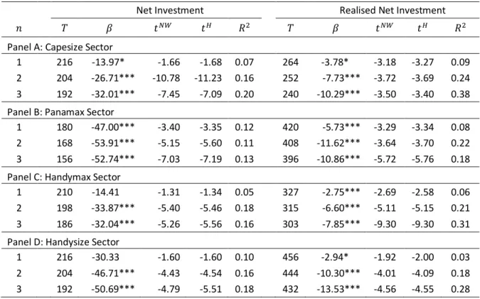
Once again, we scale the investment variable by the fleet size at the beginning of period 𝑡 → 𝑡 + 1. Accordingly, we perform a second set of regressions as the ones in equation (21), using realised net investment as the explanatory variable. The results in Table 7 suggest that current net investment negatively predicts future net earnings growth. Interestingly, we observe that there is a big spike in the significance and magnitude of the slope coefficients in the 2-year horizon which we believe reflects the time lag required for the delivery of a newbuilding order.

Table 7: Regressions of future net earnings growth on current net investment.

Net Investment Realised Net Investment

𝑛 𝑇 𝛽 𝑡•– _𝑡´ _𝑅[ _{𝑇 𝛽 𝑡}•– _𝑡´ _𝑅[

Panel A: Capesize Sector

1 216 -13.97* -1.66 -1.68 0.07 264 -3.78* -3.18 -3.27 0.09 2 204 -26.71*** _{-10.78 -11.23 0.16 252} -7.73*** -3.72 -3.69 0.24 3 192 -32.01*** -7.45 -7.09 0.20 240 -10.29*** -3.50 -3.40 0.38 Panel B: Panamax Sector

1 ₁₈₀ -47.00*** -3.40 -3.35 0.12 420 -5.73*** -3.29 -3.34 0.08 2 168 -53.91*** -5.15 _{-5.60 0.11 408} -11.62*** -3.64 -3.70 0.22 3 156 -52.74*** -7.03 -7.19 0.13 396 -10.86*** -5.72 -5.76 0.18 Panel C: Handymax Sector

1 _{210 -14.41} -1.31 _{-1.34 0.05 327} -2.75*** -2.69 -2.58 0.06 2 198 -33.87*** -5.40 _{-5.46 0.18 315} -6.60*** -5.11 -5.15 0.21 3 ₁₈₆ -32.04*** -5.26 _{-5.56 0.16 303} -7.85*** -9.30 -9.30 0.31 Panel D: Handysize Sector

1 216 -30.33 -1.60 _{-1.60 0.10 456 -2.94*} -1.92 -2.00 0.03 2 204 -46.71*** -4.43 -4.54 0.16 444 -10.30*** -4.01 -4.09 0.18 3 192 -50.69*** -4.79 _{-5.51 0.18 432} -13.53*** -4.56 -4.55 0.28

Notes: This table reports results from 1-, 2-, and 3-year horizon forecasting regressions of real log net earnings growth on current net investment and realised net investment. The data for the net investment regressions start from January 1996 while the data for the realised net investment are from January 1976. We use the Newey-West (1987) HAC (t˜™_{) and Hodrick}

(1992) (tµ_{) corrections to account for the overlapping nature of returns. *, **, or *** indicate significance at the 10%, 5% or}

In conclusion, market participants are, at least partially, anticipating this mechanism and value second-hand vessels expecting future net earnings to decrease compared to their prevailing levels. Thus, current net earnings, through current investment, have a negative SOE on current second-hand prices and, in turn, the growth rate of net earnings is higher than the one of vessel prices. Consequently, net earnings are more volatile than vessel prices and earnings yields are strongly positively related with both current net earnings and prices but negatively related with future market conditions. Since valuation ratios are used as indicators of the fundamental value of the asset relative to the generated cash flow (Campbell and Shiller, 1988b), we can argue that vessels are relatively undervalued when freight markets are very strong and vice versa.

While our results are in line with recent findings from the majority of international (Rangvid et al, 2014) and the pre-WWII U.S. (Chen 2009) equity markets, they are different to the ones from the Germany, UK, and post-WWII U.S. equity markets (Cochrane, 2011). In the latter case, the dividend yield is strongly and positively associated with future returns while future dividend growth appears to be unpredictable.

Since though, one might argue that equities are a financial asset class while vessels a real one, we also compare our respective findings with the real estate markets. Namely, regarding residential and commercial real estate, Hamilton and Schwab (1985) and Gallin (2008) find a strong negative relation between the rent yield and future rent growth. Ghysels et al (2012) estimate predictive regressions of future returns on the current rent yield and their results suggest that returns are statistically insignificant; they also find that cash flow predictability is much stronger than predictability of returns. In line with Plazzi, Torous, and Valkanov (2010), predictability is stronger in the commercial part of the industry which is arguably closer to shipping markets. Thus, the question of interest is what drives the observed similarities and differences across different industries and stock markets.

Research in equity markets suggests that dividend predictability increases with dividend volatility or, equivalently, decreases with dividend smoothing. Fama and French (1988) find that in the post-WWII period, U.S. stock returns are at least 2.4 times more volatile than dividend changes, that is dividends are smoother compared to stock prices. Similarly, Chen et al (2009) show that dividend smoothing is more widespread in the U.S. stock market, especially in the post-WWII period. Dividend smoothing increases the persistence of dividend yields and expunges the predictability of future dividend growth since it disentangles dividends from fluctuations in dividend yields. In other words, in the absence of dividend smoothing, dividends depend on the corresponding earnings and their predictability increases accordingly. In this case, a high current dividend has a negative SOE on current prices and vice versa. In turn, current dividend yields strongly and negatively predict future dividend growth. In line with this argument, Rangvid et al (2014) show that predictability is stronger in countries

where dividends are less smooth, the typical firm is small, and volatility is higher; that is in relatively small and less developed markets. Since net earnings are the natural analogue in shipping of dividends in equity markets, the argument above is in line with the empirical results presented in this paper.

In conclusion, the degree of cash flow predictability by the valuation ratio depends on the magnitude of SOEs of current cash flows on future cash flows. Since current asset prices reflect the expected cash flows to be generated by the asset, the more powerful the SOEs are, the more predictable future cash flows become and, the more informative prices and the valuation ratio are about future market conditions. Similarly, in the absence of SOEs, future cash flows should not be predictable by the current valuation ratio. In other words, if future cash flows are not economically predictable using the time 𝑡 information filtration then they cannot be predicted by valuation ratios.

The same argument applies to the real estate industry as well. Abraham and Hendershott (1996) find that rent growth predictability in residential markets is positively related to supply elasticity (e.g. the availability of land to build). Furthermore, Wheaton and Torto (1988) illustrate a strong relationship between future rent growth and current excess vacancy. Namely, for a given shock in current rents, the higher the elasticity of local supply, the stronger the SOEs become on future rents and on current real estate prices.; as a result, the predictability of future market conditions from the current rent yield increases accordingly. The results in Table 7 suggest that this is also the case in the shipping industry. Namely, the higher the elasticity of shipping supply – approximated by current or realised net investment – the stronger the SOEs on future net earnings and thus, the higher the predictability of future market conditions from the earnings yield.

V.

Conclusion

This article analyses the relation between second-hand vessel prices, net earnings, and holding period returns in the Capesize, Panamax, Handymax, and Handysize sectors of the dry bulk shipping industry. In order to determine the main driver of vessel prices, we incorporate the Campbell-Shiller (1988b) variance decomposition framework.

We show that high shipping earnings yields strongly and negatively predict future net earnings growth. Furthermore, there is no consistent evidence of time-varying expected returns in the second-hand dry bulk shipping industry. Equivalently, it seems that ship prices mainly vary due to news about expected market conditions per se and not due to news about the terminal scrap price of the vessel or because shipowners, when valuing vessels, require time-varying risk premia. These arguments are further reinforced using the Campbell-Shiller (1988a) VAR framework. To the best of our knowledge, those stylised facts had never been documented before in the shipping literature.