CAEPR Working Paper
#004-2010
Backtesting Value-at-Risk Models: A
Multivariate Approach
Cristina Danciulescu
Indiana University
April 3 2010
This paper can be downloaded without charge from the Social Science Research Network
electronic library at: http://ssrn.com/abstract=1591049.
The Center for Applied Economics and Policy Research resides in the Department of Economics
at Indiana University Bloomington. CAEPR can be found on the Internet at:
http://www.indiana.edu/~caepr
. CAEPR can be reached via email at
[email protected]
or
via phone at 812-855-4050.
©2008 by NAME. All rights reserved. Short sections of text, not to exceed two paragraphs, may
be quoted without explicit permission provided that full credit, including © notice, is given to
the source.
Backtesting Value-at-Risk Models: A Multivariate
Approach
Cristina Danciulescu
Indiana University Bloomington
This draft, April 3rd, 2010
Abstract
The purpose of this paper is to develop a new and simple backtesting procedure that ex-tends the previous work into the multivariate framework. We propose to use the multivariate Portmanteau statistic of Ljung-Box type tojointly test for the absence of autocorrelations and cross-correlations in the vector of hits sequences for different positions, business lines or financial institutions. Simulation exercises illustrate that this shift to a multivariate hits dimension delivers a test that increases significantly the power of the traditional backtesting methods in capturing systemic risk: the building up of positive and significant hits cross-correlations which translates into simultaneous realization of large losses at several business lines or banks. Our multivariate procedure is addressing also an operational risk issue. The proposed technique provides a simple solution to the Value-at-Risk(VaR) estimates aggregation problem: the institution’s global VaR measure being either smaller or larger than the sum of individual trading lines’ VaRs leading to the institution either under- or over- risk exposure by maintaining excessively high or low capital levels. An application using Profit and Loss and VaR data collected from two international major banks illustrates how our proposed testing approach performs in a realistic environment. Results from experiments we conducted using banks’ data suggest that the proposed multivariate testing procedure is a more powerful tool in detecting systemic risk if it is combined with multivariate risk modeling i.e. if covariances are modeled in the VaR forecasts.
Keywords and Phrases: Risk Management, Value-at-Risk, Backtesting, Multivariate Testing, Systemic Risk, Operational Risk.
JEL classification code: C12, C32, C52, G28, G32.
1 2
1Corresponding author: Cristina Danciulescu, Department of Economics, Indiana University, Wylie Hall 105, 100 S.
Woodlawn, Bloomington, IN 47405. E-mail: [email protected].
2I am indebted to my adviser, Professor Juan Carlos Escanciano, for his valuable advice, guidance and support
during the formation of this paper. I am, also, thankful to Christophe Perignon and Daniel R. Smith for sharing their collected data from the paper “The Level and Quality of Value-at-Risk Disclosure by Commercial Banks” to be used in the application section of this paper, Craig W. Holden, Joon Y. Park, Yoosoon Chang, Yoon-Jin Lee, and Econometrics seminar participants at Indiana University Bloomington for helpful comments. All errors are mine.
1
Introduction
Trading accounts of large financial institutions have grown very rapidly and became progressively more complex. Nowadays, their global portfolios contain several thousands positions with thousands of market risk factors as for example interest rates, equity, exchange rates, over-the-counter derivatives, commodity prices, etc.3 In this context, in order to properly manage market risks, major trading banks
developed risk measurement models that aggregate these risks in current positions. For assessing risk, these models employed a standard risk metric, Value-at-Risk (VaR), which is the amount lost on a portfolio or investment with a given small probability over a fixed period of time. In statistical terms, VaR is a quantile measure which, at a given confidence levelα, describes the loss that can occur due to the exposure to the market risks over a given time period. The popularity of this measure among practitioners was due to its conceptual simplicity: the summary of many complex bad outcomes in a single monetary account.
From the regulation side, VaR models have been sanctioned by the Basel Committee in 1996 for determining the market risk capital requirements through the internal models. The measure was motivated by the proliferation of the so-called off-balance-sheet products in the banking sector in early ’90, and the necessity to find and implement risk measures that could potentially allow proper risk management for these new products. Since then, VaR has become the standard measure for the financial market risk. Regulations stipulate that estimates are to be calculated for a 99 percent lower critical value of the bank’s aggregate trading Profit and Losses (P&L) with a one-day horizon. The forecasts provide a lower bound on aggregate trading P&L that should not be breached more than 1 day in 100.
The daily VaR estimates are maintained by the banks for the purpose of forecast evaluation or “backtesting”. The backtesting procedure is the standard assessment of VaR models consisting in esti-mating ex-post the precision of the VaR forecasts. Regulatory authorities require that VaR estimates be calculated with the same risk model used for internal measurement of trading risk. Regulation does not recommend any particular backtesting procedure, though the choice of the validation technique is a key issue for the financial institutions risk management and the financial stability in general.
Traditional backtesting methods consider only univariate VaR sequences either for individual trad-ing lines or for the financial institution global portfolio. The current practice to obtain such a global VaR measure is by estimating VaRs for each portfolio or trading line, then sum all trading lines’ VaRs.4 This practice is employed due to the infeasibility of using structural models to accurately
3Berkovitz and O’Brien (2007) documented using daily U.S. bank data that banks’ trading positions are complex
and affected by non-standard risk factors, frequently rebalanced, and very different across banks.
4Perignon& Smith (2008 b) reports that banks routinely disclose their aggregate firm-level VaRs and an
increas-ing number of banks started recently disclosincreas-ing individual VaRs for each broad risk category: equity, interest rate, commodity, credit spread, foreign exchange, etc.
measure the joint distribution of all market risk factors, as well as the relationships among the risk factors and trading positions. Large banks deal on the regular basis with a very large number of positions/risk factors and they need to generate daily forecasts.5 However the problem with such
aggregation, as showed in Artzner et al. (1999) with examples in McNeil et. al (2005), is that the subadditivity property fails to hold for the VaR measure when the assets making up the positions’ portfolios have skewed distributions, a situation that can occur when there are defaultable bonds or options in the portfolios.6 7On the other hand, the solution proposed by Artzner et al. (1999) to subadditivity property failure, Expected Shortfall risk measure(ES), is difficult to backtest in practice.
8
The purpose of this paper is to propose the implementation of a new and simple multivariate VaR backtesting technique able to overcome the VaRs aggregation problem. We propose to implement a multivariate backtesting procedure applied at once to hits collected from several subgroups of positions or trading lines, where a hit or a violation corresponds to a situation in which ex-post portfolio returns are lower than VaR forecasts. More precisely, we implement a Multivariate Portmanteau test statistic of Ljung-Box type applied to hits collected from several business lines. Our proposed backtesting procedure has the advantage of exploiting a larger information set being able to capture potential business lines’ contagion or commonality in risks without the need to resort on a large and infeasible structural risk model. The method allows all the relationships among portfolios or trading lines to be tested jointly where joint testing is consistent with the notion that spillovers are the impact of global news on each market. Moreover, the proposed multivariate testing technique is easy applicable from the practitioners’ point of view. This paper shows that this shift to a multivariate hits dimension delivers a test that increases the power of the traditional backtesting methods in assessing the accuracy of VaR forecasts in the presence of systemic risk where systemic risk should be understood as the building up of positive and significant hits cross-correlations which translates into simultaneous realization of large losses at several business lines or banks. From the operational risk point of view, the multivariate procedure makes an accurate assessment of the market risks the financial institution is exposed by avoiding under- or over-risk exposure and hence maintaining excessively high or low capital levels due to the trading lines VaRs’ subadditivity property failure. Instead of adding ex-ante 5Andersen, Bollerslev, Christoffersen and Diebold (2007) documented that the size and complexity of banks trading
positions make parametric VaR methods hard to implement in practice. As many banks report to be dealing with thousands of risk factors, they choose not to attempt to estimate time-varying volatilities and covariances for the risk factors.
6Perignon& Smith (2008 b) found that the aggregate banks’ VaR may be either less or more than the sum of their
individual VaRs, hence individual VaRs are informative. In support to their findings, authors cite Deutsche Bank 2005 annual report: “Simply adding the Value-at-Risk figures of the individual risk classes to arrive at an aggregate Value-at-Risk measure would imply the assumption that the losses in all risk categories occur simultaneously”.
7As mentioned by Perignon& Smith (2008 b), Basel Committe on Banking Supervision (1996) allows banks to have
discretion in recognizing empirical correlations within and across broad risk categories when computing their aggregate VaR.
8ES is defined as the mean exceedance given the VaR is violated. Backtesting ES is difficult due to the fact that a
business lines’ VaRs (percentiles) in order to obtain the bank’s global VaR measure the test is adding ex-post hits’ autocovariances and cross-covariances which are expectations hence additive. Therefore the multivariate testing procedure coupled with multivariate risk modeling might offer an optimal solution to the operational risk problem.
We firstly introduce our proposed procedure formally, then investigate the size and power perfor-mances of the proposed method through several Monte Carlo simulations. We set up several simulation designs in order to investigate extensively the test’s power performance when spillovers among time series occur through various channels.9 Under the specifications and parameterizations considered
in this paper, we found that the multivariate testing procedure is more powerful than its univariate counterpart when cross-correlations among trading lines’ hits are positive and significant which is the case of a systemic risk development. We also found that the univariate test is more powerful than the multivariate one when cross-correlations among trading lines’ hits are negative which, from the operational risk point of view, suggests that the univariate test creates an under-risk exposure hence a loss in profitability for the financial institution by not taking into consideration potential negative co-movements or risk diversification among its trading lines.
An application using data from two major international banks investigated how our proposed backtesting method performs in a realistic environment. From the application part we found that, using a multivariate generalized autoregressive conditional heteroscedastic model, BEKK (1,1,1)10
to obtain the banks’ VaR forecasts instead of the Historical Simulation method that the two banks used, the multivariate test becomes significant at 1% and 5% over certain trading days rolling windows while the univariate tests do not. The result is consistent with our Monte Carlo findings which implied that the multivariate procedure is more powerful than the univariate one in assessing the underlying market risks a bank is exposed when markets co-move. On the other hand, with our proposed more powerful multivariate backtesting technique it is still hard to reject Historical Simulation obtained VaR forecasts. This might be due to the restriction this technique imposes on the estimation. Historical Simulation method assumes that assets are independent and identically distributed (i.i.d.) which is not the case of the financial data. We also found that, tough we have an identified event in the data, the 2001 9/11 event, the multivariate test does not become significant over the respective trading window or year but two years latter. Our intuition for getting this result is that this might be due to the presence of forward looking components as for example bonds in trading lines’ portfolios. Our work in progress is addressing this issue by incorporating market expectations or market sentiment in risk models.
An important consequence of using our backtesting approach is that capital requirements will be 9We refer to time series spillovers as defined in Hong et al. (2009), i.e. the risk of a given asset depends on the
previous risk of other asset. For more details regarding time series spillovers and their connections with the time series covariances and correlations see Hong et al. (2009).
10See Engle and Kroner (1995) for model description. Multivariate GARCH models specify the risk of one asset as
increased only when the dependencies/positive correlations among trading lines, hence hits sequences, become sufficiently important to be taken into consideration given a certain coverage probabilityα. Therefore trading floor risk managers will not have to face excessive idle capital problem, on one hand, while, on the other hand, they will have higher chance to avoid huge losses and failures due to the systemic risk. In our set up, trading line managers get an informational advantage that comes from exploiting the multivariate framework.
The remainder of this paper is organized as following. In Section 2 we describe the environment and introduce our multivariate proposed backtesting procedure. The size and the power performance of the test are examined by Monte Carlo simulations in Section 3. Section 4 applies our test to real banks’ data, and Section 5 concludes.
2
A multivariate approach to backtesting procedure: General
theory
This section defines the VaR problem in the context of a financial institution with multiple business lines or trading positions, formulates the institution forecast evaluation problem, then introduces formally the proposed multivariate backtesting method.
2.1
Financial institution with multiple trading lines: Environment
descrip-tion
Within the lines of Escanciano and Olmo (2009 a& b), we formalize the financial institution with multiple trading lines problem as follows. Suppose thatYh
t , is theh-th trading line return time series
of a certain financial institution whereh= 1, ..., H, and assume that at timet−1 the information set of this trading linehis given byWh
t−1. Let Fht−1be theσ-algebra generated byWth−1. Assuming that
the conditional distribution ofYthgivenWth−1,Fth(., θ0h, Wth−1), is continuous with a strictly increasing cumulative distribution function (c.d.f.), we define theα-th conditional VaR ofYh
t givenWth−1 as the
Fht−1measurable functionqhα(Wth−1) satisfying the equation:
P(Yth≤qαh(Wth−1)|Wth−1) =α, (1)
almost surely (a.s.),α∈(0,1),∀t∈Z.
In this paper we will consider only parametric VaR models, meaning thatqhα(Wth−1) =mhα(Wth−1, θ0h) a.s. for some θh
0 ∈ Θ, where mhα(Wth−1, θh0) is the parametric VaR model, i.e. the inverse of
Fth(., θh0, Wth−1) at the level ofαwith respect to the first argument.
Equation (1) implies that the parametric VaR for trading line h,mh
α(Wth−1, θh), is correctly specified
if and only if
a.s. for some θh
0 ∈ Θ where It,αh = 1(Yth ≤ mhα(Wth−1, θh)), and 1(A) is the indicator function, i.e.
1(A) = 1 if the eventAoccurs and 0 otherwise. The variableIt,αh is called “hit” or “exceedance”.
2.2
Forecast evaluation problem
Traditional backtesting procedures are based on testing some implications of equation (2) for the individual trading lines, h, or bank’s aggregate portfolio. If we define the financial institution aggregate returns as Yt = P
H h=1Y
h
t and the aggregate α-conditional VaR of Yt given Wt−1, the institution
information set, asqα(Wt−1) =P H h=1q h α(W h
t−1), then equation (2) for the aggregates becomes
E[It,α(θ0)|Wt−1] =α, (3)
a.s. for some θ0 ∈ Θ, where It,α = 1(P H h=1Y h t ≤ PH h=1q h
α(Wth−1)). However, since subadditivity
property does not necessarily hold for VaR measure, as already investigated by Artzner et al. (1999), this type of aggregation is problematic.
The most popular implication of the equation (2) for the univariate case is explored by Christof-fersen (1998) which is
E[It,α(θ0)|I˜t,α(θ0)] =α, (4)
a.s. for someθ0, where ˜It,α(θ0) = (It−1,α(θ0), It−2,α(θ0)...)0.
This condition is equivalent to {It,α(θ0)} being independent and identical distributed (i.i.d.)
Bernoulli random variable with parameter α, (Ber(α)). Therefore, the problem of evaluating the accuracy of VaR forecasts can be reduced to the problem of examining the unconditional coverage and independence properties of the univariate hits sequence,{It,α(θ0)}. Testing forE[It,α(θ0)] =αis
called the unconditional backtesting and testing for{It,α(θ0)}being i.i.d.is called the independence
test.
Berkovitz et al. (2006) outlined an unified approach of VaR assessment based on the fact that the unconditional coverage and independence hypotheses are both consequences of the martingale difference hypothesis for the hits process. They noted that the univariate de-meaned hits sequence,
{It,α(θ0)−α}, forms a martingale difference sequence (m.d.s), and this implies that the hits sequence
is uncorrelated at all leads and lags. On this basis, authors proposed a univariate test of the Ljung-Box type that considers the nullity of the firstK autocorrelations for the hits sequence.
If we denote byγk the univariate hits sequence autocorrelation of orderk, then to test if γk = 0
holds for the firstK autocorrelations, we have
LB(K) =T(T+ 2) K X k=1 ˆ γ2 k T−k (5)
which is, under some regularity condition11, asymptotically aχ2withKdegrees of freedom asT → ∞.
This procedure, which considers the empirical autocorrelation of order K for the hits sequence, is an improvement compared with Christoffersen (1998) test which only considered the autocorrelation of order one.
Our paper’s main assumption is that, if past hits from one trading line h is in the information set of the others, i.e. Ith−k ∈ Wti−1, ∀k ≥ 1, ∀i, ∀h, i 6= h, with i, h ∈ H and It,αi = 1(Yti ≤
mi
α(Wti−1, θi)), then the joint VaRs validation for the H trading lines using a multivariate version
of the Ljung-Box test statistic will significantly improve the validity checking of the models. More specifically, if instead of using for testing univariate hits sequences from each trading line h ∈ H
or the bank’s aggregate hits sequence, we stack all hits sequences in anH dimensional vector, i.e.
It,α(θ0) = [It,α1 (θ01), ..., It,αH(θH0 )]0, then the problem of evaluating the accuracy of VaR forecasts imply
testingjointly for the unconditional coverage and independence properties of theH dimensional hits vector,It,α(θ0), for some θ0 = [θ10, ..., θ
H
0]0 ∈ Θ. The unconditional coverage test implies testing for
E[It,α(θ0)] =α, whereαhere denotes the vector of coverage probabilities. The independence property
implies checking, in addition to the previous used tests, for
E[(It,αi (θ0i)−α)(Ith−k,α(θ0h)−α)] = 0, (6)
∀i= 1, ..., H,∀h= 1, ..., H wherei6=hand k= 1, ..., K lags.
In other words, this means that, if each trading line V aRh = mhα(Wth−1, θh) model is correctly
specified, and there is no commonality in risks, then past observations from a business line hits sequence should not help predict future violations of itself or violations for other business lines.
2.3
Backtesting procedure using a multivariate Portmanteau test statistic
Our proposed backtesting method is based on the multivariate Ljung-Box statistic. The test takes into considerationboth the autocorrelations and cross-correlations among hits sequences for trading lines under consideration or supervision. The procedure is a joint test for the unconditional coverage and independence properties using violations from several business lines at once, henceexploiting a larger information set than the previous methods.
LetIt,α(θ0) be the H-dimensional vector of the trading lines violations series as defined in the
pre-vious section. If we denote by Γk the population covariance matrix, Γk =E[(It,α(θ0)−α)(It−k,α(θ0)−
α)0], and byD anHxH diagonal matrix with standard deviation of Ih
t,α(θh0) on the main diagonal,
then by analogy with the univariate case, we can define the lag-kcross-correlation matrix of It,α(θ0)
as
ρk=D−1ΓkD−1, (7)
with its (i, h)-th element given by
ρihk = γ ih k p γii 0γ0hh , (8)
∀i= 1, ...H,∀h= 1, ...Htrading lines, and∀k= 1, ...Klags. Whenk= 0 we get the contemporaneous cross-correlation matrix ofIt,α(θ0).
The multivariate testing procedure is carried out in out-of-sample exercises. The forecast environ-ment can be described as following. LetYt={Yt1, ..., YtH}, and suppose that{Yt, Z
0
t}Tt=1of sizeT ≥1
are used to evaluateV aR={V aR1, ..., V aRH}forecasts, where here Ztdenotes other economic and
financial variables from the information set. Assuming that the first R observations in each trad-ing line sample are used to estimate the parameters for the respective VaR model, then it remains
P =T −Rpredictions to be evaluated for each htrading line. West and McCracken (1998) consid-ered, for example, three forecasting schemes: recursive, rolling, and fixed. They differ depending on howθh
0 are estimated. In the recursive scheme, the estimators ˆθht are computed with all the sample
available up to timet. In the rolling scheme only the lastRvalues of the series are used to estimate ˆ
θht, which means that they are constructed from the samples=t−R+ 1, ..., T. In the fixed scheme the parameters are not updated when new observations become available, meaning that ˆθh
t = ˆθhR, for
allt,R≤t≤T. In the current set up we will only consider the fixed forecasting scheme for the sake of computational simplicity.
In the backtesting context, the ih-th element of the hits covariance matrix at different lagsk is defined as
ξP,kih =Cov(It,αi (θ0i), Ith−k,α(θ0h)), k≥1, (9)
∀i= 1, ...H, ∀h= 1, ...H, and can be consistently estimated under E[It,αi (θi0)] =α, E[It,αh (θh0)] =α
by γP,kih = 1 P−k T X t=R+k+1 [(It,αi (θi0)−α)(Ith−k,α(θh0)−α)], k≥1. (10) Analogously, the sample covariance of the multivariate hits vector is given by
ΓP,k= 1 P−k T X t=R+k+1 [(It,α(θ0)−α)(It−k,α(θ0)−α)], k≥1. (11)
Alternatively, if we use the hits correlation matrix for testing, itsih-th element is defined in our backtesting framework as ρihP,k= γih P,k q γii P,0γP,hh0 . (12)
The univariate Ljung-Box statistic applied to univariate hits sequences can be generalized to the multivariate case. The implementation of the multivariate test consists, for a given lag lengthK≥1, in testing the null hypothesis corresponding to the joint nullity for correlation of orderkin the hits vectorIt(θ0), wherek= 1, ..., K.
The null hypothesis of the test statistic is
H0:ρ1=ρ2=...=ρK= 0, (13)
and the alternative hypothesis is
H1:ρk 6= 0, (14)
for somek= 1,2, ..., K.
However, in practice tests for (13) are based on estimates of the relevant parameters such as
ˆ γihP,k= 1 P−k T X t=R+k+1 [(It,αi (ˆθti−1)−α)(Ith−k,α(ˆθht−k−1)−α)], (15) ˆ ΓP,k= 1 P−k T X t=R+k+1 [(It,α(ˆθt−1)−α)(It−k,α(ˆθt−k)−α)], (16) respectively ˆ ρihP,k= ˆγ ih P,k q ˆ γii P,0ˆγP,hh0 . (17)
The proposed multivariate Portmanteau statistic tests for the absence of autocorrelations and cross-correlations between pairwise hits sequences, jointly, and in terms of sample covariance matrices takes the following form:
QH(K) =P(P+ 2) K X k=1 1 P−ktr(ˆΓP,k ˆ ΓP,−10ΓˆP,kΓˆ−P,10), (18)
whereP is the size of the predicted interval,K≥1 is the considered lag length, H is the dimension of the vector of hits considered,It(θ), andtr(A) is the trace of the matrix A.
In terms of sample correlation matrices, the test statisticQH(K) can, also, be written as
QH(K) =P(P+ 2) K X k=1 1 P−krˆ 0 P,k( ˆρ− 1 P,0⊗ρˆ −1 P,0)ˆr 0 P,k, (19) where ˆrP,k =vec( ˆρ 0
P,k),vec(A) denotes the vectorization of the matrix A and⊗ denotes Kronecker
product operation.
The modification of this test statistic recommended for samples of moderate size by Li and McLeod is given by Q∗H(K) =P K X k=1 1 P−krˆ 0 P,k( ˆρ− 1 P,0⊗ρˆ −1 P,0)ˆr 0 P,k+ H2K(K+ 1) 2P , (20)
2.4
Asymptotic theory
In order to derive the limit distribution for our proposed test under the null hypothesis, we need to impose a set of regularity conditions on the data generating process for Yth, the VaR models
mh
α(Wth−1, θh), the parameter estimators ˆθht, and the ratio between the size of the estimation sample,
R, versus the prediction sample,P,π= P
R. A detailed description of the conditions and assumptions
we make can be found in the Appendix.
The derivation of the limit distribution of the test is complicated by the fact that we do not observe the true parameters value,θ0h, hence we have to estimate them. For the consequences of ig-noring parameter uncertainty and the ways to correct the limit distributions of the current backtesting methods in use see Escanciano&Olmo (2008 a&b). Alternatively, one can proceed assuming that the estimation ofθh
0 by ˆθthhas no effect on inference as the existing literature assumed with the exception
of Escanciano&Olmo (2009 a&b). Note that this assumption is valid only if the sample size used for estimating the parameters,R, is much larger than the prediction sample,P. Under this circumstance, replacingθh
0 with ˆθht has no impact on the limit distribution of the test,QH(K). In this paper, we
derive the limit distribution ofQH(K) under this assumption. This assumption greatly simplifies the
construction and implementation of the proposed multivariate test because we do not need to know the asymptotic expansion of ˆθh
t and can choose any √
T-consistent estimator.
Theorem 1: Under the Assumptions A1-A5 in the Appendix, under H0
QH(K)→dχ2(KH2), (21)
asT → ∞, whereK is the lag length andH is the number of trading lines considered.
3
Monte Carlo simulations
In this section we examine the finite sample performance of our proposed test through several Monte Carlo simulations. The aim of the exercises is to asses the empirical size (probability of incorrectly rejecting the null hypothesis) and power (probability of rejecting a false null) for the multivariate test. We used several data generating processes (DGPs) so that we can investigate extensively what are the potential gains and drawbacks from applying the proposed multivariate testing procedure under various realistic environments.
In our Monte Carlo experiments we investigate both the influence of the lag order K and out-of-sample size choicesP. For the sake of computational simplicity we report results only for the fixed forecasting scheme withπ= PR = 0.0512 13, whereRis the in-sample size, andP is the out-of-sample
12Our choice value forπis motivated by our assumptions, see the Appendix.
size to be forecasted. For all simulations we considered the out-of-sample sizesP = 250,500 for which the in-sample sizes implied by imposingπ= PR = 0.05 are R= 5000,10000. The choices for the lag lengths areK= 1,5,10,15.14
The first Monte Carlo design follows the one proposed by Christoffersen (1998). He modeled the violations process by a Markov chain with transition probabilities:
Π = p00 p01 p10 p11 . (22)
Under the null hypothesis (H0), the violations have a constant conditional mean which implies the
linear restriction p00 = p10 = α. Hence, the probability of having a violation at time t is equal
with α, the coverage rate, no matter the state at t−1. Under the alternative hypothesis (H1),
pij =P[It,α(θ0) =j|It−1,α(θ0) =i]6=α. The Markov chain reflects only the existence of a correlation
of order one in the process of hits sequence, It(θ0). This means that the probability of having a
violation (respective not having one) for the current period depends only on the occurrence of a violation or not for the same level of coverageαin the previous period.
For our multivariate case we generated, under the null, two uncorrelated Markov chains for which the violations for both have a constant conditional mean which implies the linear restriction p1
00 =
p1
10=p200=p210 =α, where the superscript indicates the chain. Under the alternative hypothesis we
maintained the linear restriction but we generated correlated chains with cross-correlation set at 0.9. We consideredα= 1%, 5% and 10% corresponding to hits sequences with shortfall probabilities or risk levels of 1%, 5% and 10%.
The Monte Carlo algorithm’s main steps in this design are as following:
1. GenerateR+P observations for eachhbinary (hits) sequence (we will get a matrix ofH hits), 2. Implement the proposed multivariate test for the obtained matrix of hits sequences and compare it with aχ2(H2K),
3. Implement the univariate test for each univariate hits sequence and compare with aχ2(K),
4. Repeat the previous steps for l times and calculate the rejection rates. Rejection rates are calculated overl= 1000 Monte Carlo trials.
The advantage of considering this design is that estimation effects do not affect the limit distribu-tion of the tests. The draw back is that it captures only the correladistribu-tion of order 1.
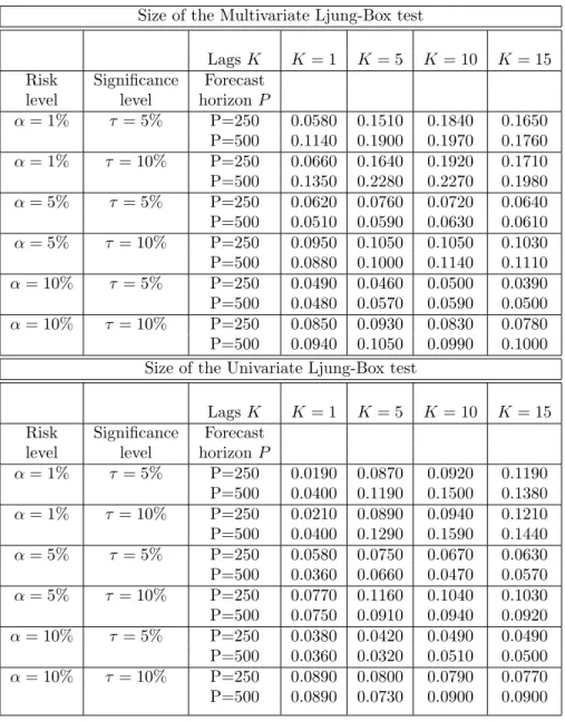
Table 1 displays simulation results for the size of the multivariate test and its univariate counter-part. For the size of the test, if the asymptotic distribution is accurate in the sample sizes considered, the rejection frequencies should be close to the nominal size of the test which we set to be either
procedures’ asymptotic distribution.
14The choices for lag lengths are in line with Chitturi (1974) assumption. The author derived the asymptotic
τ = 5% or τ = 10%. We found that the size of the multivariate test is close to the nominal values considered of 5% and 10% for the risk levels α= 5% and α= 10%. On the other hand the test is oversized forα= 1% risk level. This result is not new in the literature. Escanciano and Olmo (2008 a) obtained similar results for their Monte Carlo experiments and they suggested that this problem may be intrinsic to VaR inferences at low quantile levels and not to the existence of the estimation risk. This problem is also investigated extensively in Danciulescu (2010 b).
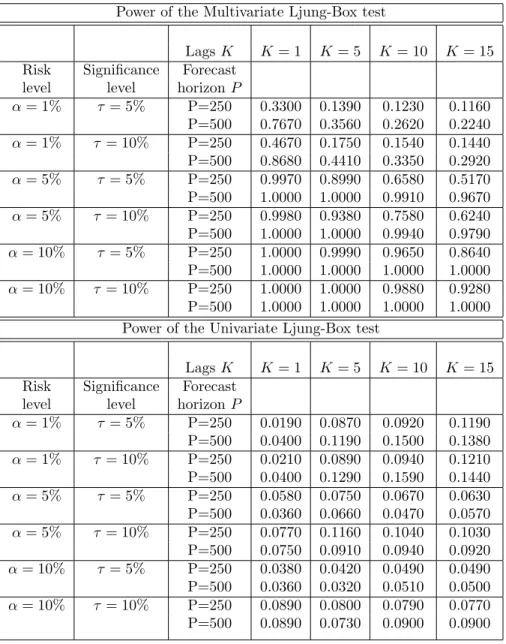
Table 2 shows results for the power simulations under this Monte Carlo design. Our results illustrate a significant increase in power in moving from the univariate to a multivariate testing environment. The power of the test is increasing in the out-of-sample size P and decreasing with the lag length K over all significance and risk levels considered. The latter is expected since all the correlation is at the first lag.
For our second Monte Carlo exercise we employed Hong et al. (2009) nested GARCH DGP to simulate returns forhtrading lines. We decided to use this DGP since GARCH is the most common specification for modeling financial returns. In our simulations we considered only H = 2 as the authors did. Hong et al. (2009) DGP allowed us to disentangle and investigate separately the channels through which spillovers among the business lines’ returns may occur. In this paper we investigated only the spillovers that may occur through the time series’ means and variances.
The nested GARCH DGP is specified as following:
Yht=βh1Y1t−1+βh2Y2t−1+uht, (23)
uht=σhtεht, (24)
σ2ht=γh0+γh1σ2ht−1+γh2u21t−1+γh3u22t−1, (25)
εht∼m.d.s., (26)
We assumed that innovations,εht, arei.i.d tν standardized disturbances i.e. εht=
q
ν−2
ν ∗vhtwith
vhtdistributed as a Student-t withν degrees of freedom forh= 1,2.
Using Hong et al. (2009) DGP we investigated both the size and the power of the proposed multivariate test. The values of the parameters are obtained by fitting GARCH models to the banks’ daily returns data we used in the application part of the paper.
We assessed the size of the test under the null (H0) using the following parameter values:
(β11, β12, γ10, γ11, γ12, γ13) = (0,0,0.05,0.88,0.01,0), (27)
(β21, β22, γ20, γ21, γ22, γ23) = (0,0,0.15,0.73,0,0.1). (28)
The innovation processes,εht, are assumed to follow a Student-t distribution withνh = 5 degrees of
freedom forh= 1,2. Our choice for the innovations’ distribution and degrees of freedom parametriza-tion is motivated by Perignon & Smith (2009 a) estimaparametriza-tion results. Using data from around the World
fifty major banks they found that a Student-t distribution with between 5 and 8 degrees of freedom is the best choice to account for the observed data leptokurtosis.
For this Monte Carlo design, the algorithm’s main steps are as follows:
1. Using Hong et al. (2009) DGP and the true parameter values, generateR+P observations for theH trading lines,
2. Using the firstR (in-sample) observations generated, estimate the parameters of the model by quasi maximum likelihood method (QMLE),
3. Using the estimated parameters we generate the out-of-sampleP observations from univariate GARCH DGPs,
4. Get the hits sequence for each individual series of financial return generated. We will get a matrix ofH hits (H = 2 in our bivariate case),
5. Implement the proposed multivariate test for the obtained matrix of hits sequences and compare it with aχ2(H2K),
6. Implement the univariate test for the univariate hits sequence of interest and compare it with aχ2(K),
7. Repeat the previous steps forl times and calculate the rejection rates.
As in our previous Monte Carlo design we consideredl= 1000.
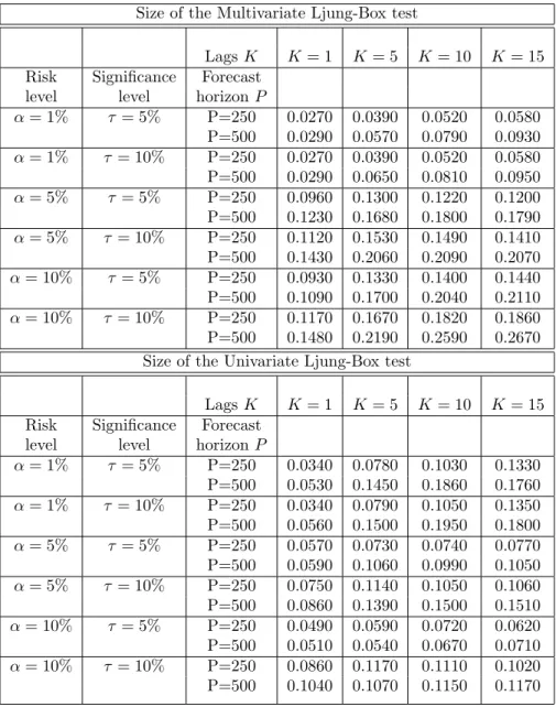
Table 3 shows the results for the size of the test using the above DGP and parametrization. We found that the multivariate test is slightly over-sized for this specification compared to the nominal values considered of 5% and 10% for the risk levelsα= 5% andα= 10% while the test is undersized for the risk level α= 1%. As in the previous Monte Carlo design for size we refer to Danciulescu (2010 b) work as a potential explanation for these size distortions.
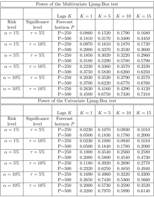
Using Hong et al. (2009) DGP with different parameter values we conducted Monte Carlo experi-ments to compare the empirical powers of the multivariate and univariate methods for rejecting some alternatives to the null. We employed parameterizations that allowed us to investigate separately the power of the test when spillovers between financial returns come through their mean (main body of the distributions) or through their variance (tails of the distributions).
We used the following parameter values to investigate the power of the test under the alternative (H1) when there are spillovers between returns through their mean:
(β11, β12, γ10, γ11, γ12, γ13) = (0,0.7,0.05,0.88,0.01,0), (29)
(β21, β22, γ20, γ21, γ22, γ23) = (0,0,0.15,0.73,0,0.1), (30)
and when there are spillovers between returns through their variance:
(β21, β22, γ20, γ21, γ22, γ23) = (0,0,0.15,0.73,0,0.1). (32)
For all cases, the innovations processesεhtare assumed to follow a Student-t distribution withνh= 5
degrees of freedom forh= 1,2.
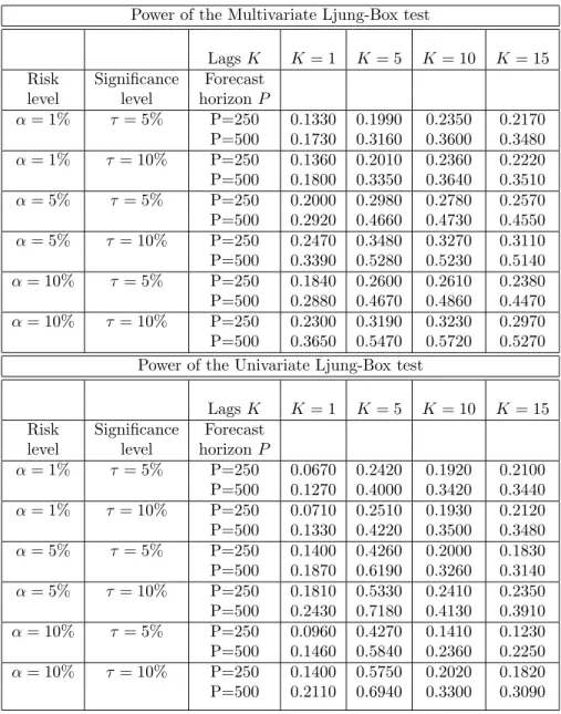
In tables 4 and 5 we report the rejection probabilities at 5% and 10% significance level for the last two parameterizations. The simulation results for the power show that in both cases, spillovers between returns through their mean and variance, we get a significant gain in power for the multivariate test versus the univariate one for the lag lengths 1, 10 and 15, while at the lag 5 the univariate test is more powerful than the multivariate one. The power of the test is also increasing in the out-of-sample size P over all significance levels considered. These findings suggest that the multivariate test is more powerful in capturing the co-movements (positive and significant cross-correlations) among the trading lines hits sequences. Also, by capturing the negative movements among trading lines (negative cross-correlations), our results suggest the multivariate test is a better choice from the operational risk point of view. Proposed procedure makes an accurate assessment of the market risks the financial institution avoiding under-risk as well as over-risk exposure and consequently maintaining excessively high or low capital levels with negative implications as decrease in bank’s profitability or its failure.
The economic intuition of this result is also of interest. A potential explanation of the negative cross-correlation at lag 5 might be due to the fact that banks might use assets (bonds) with different maturities for hedging the risk in their portfolios/business lines or different trading strategies. For example one trading line/bank is shorting the risky assets at day 5 while the other is holding risky assets longer in its portfolio.
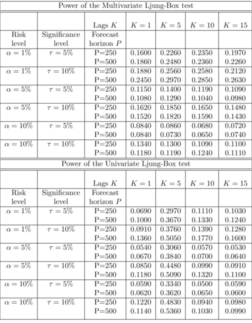
The third Monte Carlo design investigates the power of the multivariate testing procedure using data generated from a bivariate BEKK process as introduced by Engle and Kroner (1995). This specification is recommendable for modeling the dynamic correlation structure among different trading lines (risk categories) as recommended in the Amendment of the Basel Accord (1996).15 Moreover,
BEKK model is a more realistic representation of the financial markets environment with spillovers among time series that occur through various channels without the possibility to clearly identify them. In this set up financial returns are modeled as a multivariate stochastic vector process{Yt}with dimensionHx1 such thatE(Yt) = 0. The vectorYtis assumed to be conditionally heteroscedastic:
Yt=M
1/2
t εt, (33)
given the information setWt−1, whereWt−1 denotes the information set generated by the observed
series{Yt−1}up to and including timet−1. TheHxHmatrixMt= [mijt] is the conditional covariance
matrix ofYt, andεt is an i.i.d. vector error process.
The matrix processMtfor the BEKK model has the form:
Mt=A0A 0 0+ K X k=1 q X i=1 A0kiYt−iY 0 t−iAki+ K X k=1 p X j=1 Bkj0 Mt−jBkj, (34)
whereAki,Bkj, and A0 areHxH parameter matrices, withA0 lower triangular. The decomposition
of the constant term into a product of two triangular matrices is to ensure positive definiteness ofMt.
In our caseYtis a vector of H log-returns corresponding toH trading lines.
Since the number of parameters in a full BEKK model is (p+q)KH2+H(H+1), in order to reduce
the computational burden, we employed in our Monte Carlo simulations a bivariate BEKK(1,1,1), henceH = 2.
As in the case of Hong et al. (2009) design, the BEKK DGP is parametrized using values that we got by fitting the model to the banks’ data:
(a0,11, a0,21, a0,22, a1,11, a1,12, a1,21, a1,22, b11, b12, b21, b22) = (14.8511,0.6318,1.0809,0.2525,−0.2308,
−0.3709,0.0807,0.3503,0.6730,−0.4592,0.3663) (35) Innovations are assumed to follow a bivariate Student-t distribution with ν = 5 degrees of freedom, and the variance-covariance matrix elementsσ11=σ22= 1 and σ12=σ21= 0.4.
The simulation environment follows the same steps and considerations as in the case of Hong et al. (2009) DGP. The fitted risk model for each generated time series from the BEKK DGP is a GARCH(1,1).
Table 6 displays the results for this Monte Carlo experiment. Using BEKK design we get similar results for power as in the Hong et al. (2009) Monte Carlo design.
In summarizing our Monte Carlo results we conclude that our paper contributes to the exiting liter-ature by showing that in moving to a multivariate backtesting procedure from a univariate method we get a power improvement in capturing the co-movements (positive cross-correlations) among the trad-ing lines or financial institutions while avoidtrad-ing financial institution under-risk exposure by capturtrad-ing the negative movements (negative cross-correlations) among her trading lines. Hence the multivariate technique represents an improvement in testing the accuracy of VaR forecasts.
4
Application
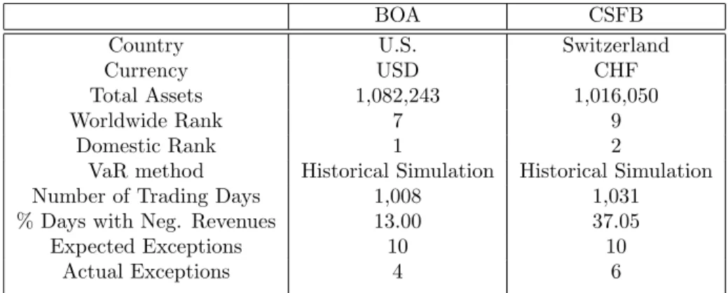
To illustrate how our new proposed backtesting procedure works in a real data environment, we apply the test to two international major banks’ P&L and VaR data. The sample was made available to us by Christophe Perignon and Daniel R. Smith, who developed in Perignon& Smith (2009 a) a method to extract one day-ahead VaRs and daily trading revenues data from the graphs disclosed by the banks. The authors selected a sample of five large banks from five different countries and collected annual 10-K forms from the SEC-EDGAR website, annual reports from the banks’ websites or hardcopies from the banks, for the period 1995-2005. They focused on the largest banks since presumably large banks devote the most resources to computing VaRs. 16
From their sample of five banks we chose for our analysis Bank of America and Credit Suisse First Boston Bank. In their annual statements the two financial institutions report actual revenues that are affected by their intraday trades. Banks’ trading revenues are based on position values recorded at the close of the day and represent the banks’ consolidated trading activities. The usual activities include trading in interest rate, foreign exchange, equity assets, liabilities, and derivative contracts. Perignon&Smith (2009 a) reports that, for these two banks, it is not stated explicitly if their trading revenues are inflated or not by trading fees or commissions, which may create some distortions in backtesting. The banks’ VaRs are calculated for a one-day-ahead-horizon and a 99% confidence level for profit and losses (P&L), that is the 1% lower tail of theirP&Ldistributions.
Figure 1 shows the graphs of the daily trading revenues and one day-ahead 99% VaRs for our selected banks. From the graphs we observe that there are fewer exceptions or days when the actual loss is greater than the VaR consistent with the one percent coverage probability. Bank of America had four exceptions and Credit Suisse First Boston bank had six exceptions over the period considered. Because there are around 1000 observations in the sample, the expected number of exceptions is 10 for both banks. The two banks differ, also, in the magnitude of violations. As one can notice from figure 1 the magnitude of violations for Credit Suisse First Boston is much higher than the ones for Bank of America.
Figure 3 plots the violation sequences for the two banks obtained using their reportedP&Land VaRs. The graph suggests that there is at best a weak relationship between the two banks’ violation sequences. Results for cross correlation between the two banks trading revenue and VaRs displayed in table 11 supports the inference made using figure 3. The correlation of their daily P&L and VaR is low. This low correlation may reflect the difference in portfolios’ composition between the two banks. Tables 9 and 10 present the summary statistics for daily P&L and VaR data for the two banks under our investigation as reported in Perignon&Smith (2009). From the descriptive statistics one can notice significant differences in average P&L, standard deviation and kurtosis between the two banks. The magnitude of trading activity is almost three times larger for Bank of America versus Credit Suisse First Boston Bank. The average daily P&L for Bank of America was 13.8698 million dollars while the average daily P&L for Credit Suisse First Boston bank was 5.0318 million dollars. Trading revenues for both banks are highly volatile with extreme profits and losses, right skewed, and exhibit ARCH effects. The P&L for Credit Suisse First Boston bank displays excess kurtosis relative to the normal distribution. The Dickey-Fuller test indicates that both banks’ trading revenues are stationary. There is also evidence of modest autocorrelation around 5 to 10 % for revenue series of both banks. The summary statistics for their VaR figures shows that they are strongly autocorrelated. The methodology used by banks to construct their VaRs is Historical Simulation. Histograms of P&L and VaRs for the two banks are presented in Figure 4.
We applied our backtesting procedure to the banks’ observed sequences ofP&Land VaRs consid-ering a 250-day moving window. Therefore, with our available data, we repeated the procedure for
a total of four different periods. That is, for the second period we considered the forecasting period fromP = 251 toP = 500, for the third period fromP = 501 toP = 750, and for the last period from
P= 751 to P = 1000.
Table 7 reports statistics for both the multivariate and univariate tests and the number of excee-dences (Vio) for the four windows. We found no rejections at 1% and 5% either for the multivariate test or for the univariate one over the windows and lag lengths considered.
We repeated the testing procedures using the observedP&L but with VaR forecasts obtained by fitting a BEKK (1,1,1) as risk model. To the best of our knowledge this is the first paper to use a multivariate risk model for obtaining the VaR forecasts. The advantage of using a multivariate risk model is capturing in VaRs not only business lines or banks’ conditional variances but also their covariances. Table 8 reports the testing results. We found that for the rolling windowP = 501 : 750 the multivariate test is significant at 1% for lagsK= 1,5,10 while the univariate tests are not. The total number of violations obtained using BEKK(1,1,1) risk model at 1 % risk level is comparable to the one obtained using banks’ reported method which is Historical Simulation.
The results obtained from our two exercises have several implications. First, they are consistent with our Monte Carlo simulations, which found that the multivariate test is more powerful than the univariate test in capturing co-movements (positive and significant cross-correlations). Second, con-sistent with Berkovitz et al. (2006) results, we found that it is difficult to reject historical simulation obtained VaRs even with the multivariate technique and this might be due to their design. Third, the multivariate testing procedure is a more powerful tool, able to capture the systemic risk if cross-correlations are modeled in the VaR forecasts. Fourth, multivariate risk modeling combined with multivariate testing procedures might be the best approach from the operational risk point of view since financial institutions and regulators would like to avoid over- as well as under-risk exposures. Multivariate methods are able to capture markets’ or institutions’ co-movements hence avoiding in-stitutions’ failures at the macro level if systemic risk builds up or a decrease in profitability at the micro level if the negative correlations among trading lines are not considered. Fifth, the presence of forward looking components in trading lines’ or banks’ portfolios, as for example bonds, suggests the incorporation of market expectations or market sentiment in risk models for accurately timing risk spillovers and contagion periods. As one could notice from table 8, tough the 2001 9/11 event belongs to the first rolling window, the multivariate test becomes significant over the third rolling window, in 2003.
The economic significance of backtesting methods and VaR forecasts derives from the fact that results are used to determine the minimum regulatory capital requirements which must be met by banks to guard against credit and market risks. The Basel Accord stipulates that a bank daily capital charge must be set at the higher of the previous day’s VaR or the average VaR over the last 60 business days multiplied by a factor, mft, i.e. CRt = mft∗max{V aR0t.01,601
P60
i=1V aR 0.01
t−i}.
previousT days, whereT = 250 in Basel Accord, but mft must not be lower than 3. Basel Accord
imposes penalties in the form of a higher multiplicative factor on banks which use models that lead to a greater number of violations than would be expected given the specified risk level of 1 %. A high capital charge is undesirable, other things equal, as it reduces banks’ profitability. Table 12 displays the penalties imposed for a given number of violations over a 250 trading days period.
Table 13 shows our calculations for the two banks’ mean daily capital charges using the two risk models to obtain the VaR forecasts. The results for capital charges are comparable for the two risk modeled. This outcome suggests that employing a dynamic model which accounts for the time varying assets’ correlation, as for example BEKK, does not lead to higher capital requirements for banks on one hand, while giving a higher chance to capture potential trading lines commonality in risks (the case of positive cross-correlations) or avoiding under-risk exposure (the case of negative correlations) on the other.
Capital requirement calculations revealed also a drawback of the risk models in use which is their backward looking feature. The lowest capital charges occurred during the period with the highest number of violations for both banks. This might have happened due to the fact that capital charges are based only on backtesting results and VaR forecasts from the previous periods in which volatilities and the number of violations were lower due maybe to more favorable market conditions. This outcome in particular is very important to be investigated in future research since insufficient capital buffers to cover the realized losses may lead to banks or financial institutions’ failures.
5
Conclusion
In this paper we proposed a new backtesting technique that exploits the informational advantage of the multivariate framework. The test is easy to implement and simulation results conducted over a relevant number of sample sizes, number of lags and specifications showed that the proposed multivariate backtesting procedure represents an improvement versus its univariate counterpart in assessing the accuracy of VaR forecasts. Multivariate testing technique allows all the relationships among trading lines to be tested jointly revealing a considerable increase in power for cross-market spillovers. Joint testing is consistent with the notion that spillovers are due to the impact of global news in each market and use of multivariate data allows analyzing markets’ interactions simultaneously.
An application of our proposed procedure to two major international banks real data confirmed the Monte Carlo results. Our findings imply that a partial disaggregation and analysis of risk on classes of risks or trading lines is recommendable to a full financial institution risk aggregation as a way to capture the complexity of financial linkages.
The results from the application part of the paper revealed, also, a drawback of the risk models in use, which is their backward looking feature, with important implications for correct calculation of banks’ capital requirements and identification of the risk spillover periods. Our current work in progress explores in this direction.
6
Appendix
ASSUMPTIONS AND MATHEMATICAL PROOFS
ASSUMPTIONS:
Assumptions 1-5 under which Theorem 1 is derived are similar with the ones in Escanciano and Olmo (2008 a and b).
Let the family of conditional distributions be defined as:
Fx(y) =P(Yt≤y|Wt−1=x), (36)
and letfx(y) be the associated conditional densities. We define theα-mixing coefficients as
α(m) =supn∈Z,B∈Fn,A∈Pn+msup|P(A∩B)−P(A)P(B)|, m≥1 (37)
where the σ-fields Fn and Pn are Fn = σ(Xt, t ≤ n), respectively Pn = σ(Xt, t ≥ n), and Xt =
(Yt, Z
0
t)0. Mixingness is the property that ensures dependence dies out with horizon.
For each trading lineh∈H we assume the following: Assumption 1: {Yh
t , Z
0
t}t∈Z are strictly stationary and strong mixing process with mixing
coef-ficients satisfyingP∞j=1(α(j))1−2
d <∞withd >2.
Assumption 2: The family of distribution functions {Fh
x, x ∈ Rdw} has Lebesque densities {fxh, x∈Rdw} that are uniformly bounded:
supx∈Rdw,y∈R|fxh(y)| ≤C (38)
and equicontinuous: for everyε >0, there exists aδ >0 such that
supx∈Rdw,|y−z|≤δ|fxh(y)−f h
x(z)| ≤. (39)
Assumption 3: The modelmh
α(Wth−1, θh) is continuously differentiable inθh (a.s.) with
deriva-tivesgh(Wth−1, θh) such thatE[supθh∈Θ0|gh(Wth−1, θh)|2]< C, for a neighborhood Θ0 ofθh0.
Assumption 4: The parameter space Θ is compact in Rp. The true parameter θh
0 belongs to
whereHh(t) are a px1 vector such thatHh(t) =R−1PR
s=1l
h(Yh
s, Wsh−1, θh0) for the fixed forecasting
scheme. We assume thatE[lh(Yh s, Wsh−1, θh0)|Wth−1] = 0 a.s., andVh=E[lh(Ysh, Wsh−1, θ0h)lh 0 (Yh s, Wsh−1, θ0h)|Wth−1]
exist and are positive definite.
Moreover,lh(Yth, Wth−1, θh) are continuous (a.s.) inθhin Θ0andE[supθh∈Θ
0|l h(Yh t , W h t−1, θ h)|2]≤
Care small neighborhoods aroundθh
0.
Assumption 5: R, P → ∞asn→ ∞, andlimn→∞PR =π, 0≤π <∞.
PROOF OF THEOREM 1:
We provide a sketch of proof for Theorem 1 using empirical process theory as in Escanciano and Olmo (2008 a) and a variation of weak convergence theorem as developed in Delgado and Escanciano (2007).
For notation simplicity we denote, forθh∈Θ,
Fth−1(θh) =FWhh t−1 (mhα(Wth−1, θh)), (40) and fth−1(θh) =fWhh t−1 (mhα(Wth−1, θh)). (41) As in Escanciano and Olmo (2008 a) we define the process
Knh(c) =√1 P n X t=R+1 [It,αh (θ0h+c(t−1)−1/2)−Fth−1(θ0h+c(t−1)−1/2)], (42) indexed byc∈CD, whereCD={c∈Rp:c≤D}, andD >0 is an arbitrary but fixed constant.
Lemma A1 in Escanciano and Olmo (2008 a) states that, under the Assumptions A1-A5, the processKh
n(c) is asymptotically tight with respect toc∈CD. Moreover it can be shown that for each
c∈CD,
E[|Knh(c)−Knh(0)|2] =o
P(1). (43)
The last equation and the asymptotically tightness ofKh
n(c) imply that if ˆcis bounded in
proba-bility, i.e. ˆc=OP(1), then
|Knh(ˆc)−Knh(0)|=oP(1). (44)
Next we apply these results with ˆc=maxR≤t≤n √
t(ˆθh
t−θ0h) whereRdenotes the in-sample size. We
need to prove that, under the fixed forecasting scheme we considered in this paper,maxR≤t≤n √
t(ˆθh t−
θh0) =OP(1) holds. Since for the fixed forecasting scheme we have |maxR≤t≤n( √ t R) R X s=1 lh(Yth, Wth−1, θh0)| ≤ |(√1 R) R X s=1 lh(Yth, Wth−1, θ0h)|=OP(1), (45)
then equation (44) holds for ˆc=maxR≤t≤n √
t(ˆθh
t −θh0), and hence we have
|√1 P n X t=R+1 [It,αh (ˆθht−1)−Fth−1(ˆθht−1)]−√1 P n X t=R+1 [It,αh (θh0)−Fth−1(θh0)]|=oP(1), (46)
whereP denotes the out-of-sample size. This imply the decomposition 1 √ P n X t=R+1 [It,αh (ˆθht−1)−α] = √1 P n X t=R+1 [It,αh (θ0h)−Fth−1(ˆθ0h)] +√1 P n X t=R+1 [Fth−1(ˆθth−1)−Fth−1(θh0)]+ 1 √ P n X t=R+1 [Fth−1(θ h 0)−α] +oP(1). (47) Using the Mean Value Theorem, and since expectation and differentiation can be interchanged, we have A1n = 1 √ P n X t=R+1 {Fth−1(ˆθht−1)−E[Fth−1(ˆθht−1)]−Fth−1(θh0) +E[Fth−1(θh0)]}= 1 √ P n X t=R+1 {ghα0(Wth−1,θ˜ht−1)fth−1(˜θht−1)−E[ghα0(Wth−1,θ˜th−1)fth−1(˜θth−1)]}(ˆθth−1−θh0), (48)
where ˜θht−1is between ˆθth−1 andθh0.
Assumptions A2 and A3 imply thatE[supθh∈Θ
0|g h0 α(Wth−1, θh)fWhh t−1 (mh α(Wth−1, θh))|]< C.
There-fore by uniform law of large numbers of Jennrich (1969, Theorem 2) and maxR≤t≤n √ t(ˆθh t −θ0h) = OP(1), we have thatA1n=oP(1). Similarly, 1 √ P n X t=R+1 {E[Fth−1(ˆθht−1)]−E[Fth−1(θ0h)]}= √1 P n X t=R+1 E[ghα0(Wth−1, θh0)fth−1(θh0)](ˆθht−1−θh0)+ 1 √ P n X t=R+1 {E[gαh0(Wth−1,θ˜ht−1)fth−1(˜θht−1)]−E[ghα0(Wth−1, θh0)fth−1(θh0)]}(ˆθth−1−θ0h) =B1n+B2n. (49)
By uniform law of large numbers andmaxR≤t≤n √ t(ˆθht −θh0) =OP(1), we have thatB2n=oP(1) holds. Hence, |√1 P n X t=R+1 [Fth−1(ˆθht−1)−Fth−1(θ0h)]−E[ghα0(Wth−1, θ0h)fth−1(θh0)]√1 P n X t=R+1 Hh(t−1)|=oP(1). (50) s
In order to proceed with the proof of theorem 1, for eachi, h∈H,i6=h, we define de process: Kn,kih (c) = √1 P n X t=R+k+1 {It,αi [θi0+c(t−1)−1/2]−Fti−1[θ0i+c(t−1)−1/2]}Ith−k,α[θ0h+c(t−k−1)−1/2], (51) indexed by c ∈ CD, where CD = {c ∈ Rp : |c| ≤ D}, k ≥1, and D > 0 is an arbitrary but fixed
constant.
Applying Lemma A1 from Escanciano and Olmo (2008 a) to the processKih
n,k(c) and following the
previous arguments we get
√ P−k( ˆξP,kih −ξihP,k) =√ 1 P−k n X t=R+k+1 [Fti−1(ˆθit−1)Ith−k,α(ˆθth−k−1)−Fti−1(θi0)Ith−k,α(θ0h)] +oP(1) =√ 1 P−k n X t=R+k+1 [Fti−1(ˆθit−1)Ith−k,α(ˆθth−k−1)−Fti−1(θ0i)Ith−k,α(θ0h)+ Fti−1(θ0i)Ith−k,α(ˆθht−k−1)−Fti−1(θ0i)Ith−k,α(ˆθht−k−1)] +oP(1), (52) whereξkih=cov[It,αi (θ0i), Ith−k,α(θ0h)] at different lagskwithk≥1, which can be consistently estimated byξih P k= 1 P−k Pn t=R+k+1[I i t,α(θi0)Ith−k,α(θ0h)−α2].
The previous expression can be rearranged as following
√ P−k( ˆξP,kih −ξihP,k) = 1 √ P−k n X t=R+k+1 Fti−1(θ0i)[Ith−k,α(ˆθht−k−1)−Ith−k,α(θ0h)]+ 1 √ P−k n X t=R+k+1 Ith−k,α(ˆθht−k−1)[Fti−1(ˆθti−1)−Fti−1(θi0)] +oP(1) = 1 √ P−k n X t=R+k+1 Fti−1(θ0i)[Ith−k,α(ˆθht−k−1)−Ith−k,α(θ0h)]+ 1 √ P−k n X t=R+k+1 [gαi0(Wti−1,θ˜ti−1)fti−1(˜θti−1)Ith−k,α(ˆθht−k−1)](ˆθit−1−θi0) = C1n+C2n+oP(1), (53) where ˜θi t−1is between ˆθti−1 andθi0.
SinceFti−1(θi0) =αa.s., the previous results imply that
C1n=αE[gh 0 α(W h t−k−1, θ h 0)f h t−k−1(θ h 0)] 1 √ P−k n X t=R+k+1 Hh(t−k−1) +oP(1), (54) and |C2n−E[gi 0 α(W i t−1, θ i 0)f i t−1(θ i 0)I h t−k,α(θ h 0)] 1 √ P−k n X t=R+k+1 Hi(t−k−1)|=oP(1), (55)
Hence, we proved that √ P−k( ˆξihP,k−ξP,kih ) =αE[ghα0(Wth−k−1, θh0)fth−k−1(θh0)]√ 1 P−k n X t=R+k+1 Hh(t−k−1)+ E[gαi0(Wti−1, θi0)fti−1(θ0i)Ith−k,α(θ j 0)] 1 √ P−k n X t=R+k+1 Hi(t−k−1) +oP(1). (56)
Furthermore we define the following quantities ˆ ξ1iP,k= √ 1 P−k n X t=R+k+1 [It,αi (ˆθit−1)−α], (57) ˆ ξ1hP,k= √ 1 P−k n X t=R+k+1 [Ith−k,α(ˆθht−k−1)−α], (58) and, similarly, defineξi1P,kandξ1hP,k withθi0and θh0 replacing ˆθit−1 and ˆθth−k−1.
Since ˆ γP,kih = 1 P−k n X t=k+1 [It,αi (ˆθit−1)−α][Ith−k,α(ˆθth−k−1)−α], (59) this implies that
√
P−kˆγP,kih =√P−kξˆP,kih −αξˆi1P,k−αξˆ1hP,k+ 2α2. (60)
The same equality holds forγih
P,k,ξP,kih ,ξi1P,k,ξ1hP,k √ P−kγP,kih = √ P−kξP,kih −αξ i 1P,k−αξ h 1P,k+ 2α 2 . (61)
Hence we have that
√
P−k(ˆγP,kih −γP,kih ) =√P−k( ˆξihP,k−ξP,kih )−α( ˆξ1iP,k−ξi1P,k)−α( ˆξh1P,k−ξ1hP,k). (62) Previous arguments imply that
ˆ ξ1iP,k−ξ1iP,k=E[giα0(Wti−1, θ0i)fti−1(θi0)]√ 1 P−k n X t=R+k+1 Hi(t−1) +oP(1), (63) and ˆ ξh1P,k−ξ1hP,k=E[gh 0 α(Wth−k−1, θ0h)fth−k−1(θh0)] 1 √ P−k n X t=R+k+1 Hh(t−k−1) +oP(1). (64)
Therefore we get that
√ P−k(ˆγP,kih −γP,kih ) =E{giα0(Wti−1, θ0i)fti−1(θi0)[Ith−k,α(θ0h)−α]√ 1 P−k n X t=R+k+1 Hi(t−k−1)}+oP(1). (65)
Corollary 3 in Escanciano and Olmo (2008 a) and our Assumption 5 imply that ˆγih
P,k→d N(0, α2(1−
α)2).
Moving to the multivariate framework, let {It,α(θ0)} be the H dimensional vector that collects
the hits sequences from allH trading lines. The multivariate hits process sample autocovariance and autocorrelation are defined as
ΓP,k= 1 P−k n X t=R+k+1 (It,α(θ0)−α)(It−k,α(θ0)−α)0, (66) and respectively as ρP,k= ΓP,kΓ−P,10, (67)
fork≥1, where both ΓP,k andρP,k areHxH matrices.
The two matrices can be stacked as 1xH2row vectors with rows stacked one next to the other as following ˜Γ0P,k= [γ11
P,k, ..., γP,k1H, ..., γP,kH1, ...γP,kHH] respectively ˜ρ
0
P,k= [ρ11P,k, ..., ρP,k1H, ..., ρHP,k1, ...ρHHP,k].
Chitturi (1974) showed that for largeP(k) the multivariate autocorrelation vector process has, approximately, a multivariate normal distribution with
E[ ˜ρ0P,k] = 0, (68) and cov[ ˜ρP,k,ρ˜ 0 P,l] . = 1 P(V ⊗V −1)δ k−l, (69)
where = denotes an approximate relationship,. ⊗denotes the direct product and δk−l denotes
Kro-necker delta with unity atk−l= 0 and zero elsewhere.
Rao (1973, p. 524) showed that if a random vector x has a multivariate normal distribution
N(0, QΣ) whereQis idempotent of rankpand Σ is positive-definite symmetric, then
x0Σ−1x∼χ2p. (70)
Chitturi (1974) and Hosking (1980, Theorem 2) completed the proofs for the multivariate autoco-variance and autocorrelation functions considering AR and ARMA processes17, hence the result from our Theorem 1 follows. Q.E.D
Table 1: Sizes of the Multivariate Ljung-Box and Univariate Ljung-Box tests for Christoffersen (1998) design. We simulatei.i.d.Bernoulli variables with the probability of having a violation at timetequal withα, the coverage rate, (i.e. p1
00=p110=p200=p102 =α). VaR is computed atα= 0.01,α= 0.05
andα= 0.10. 1000 Monte Carlo simulations were performed andπis fixed at π=P/R= 0.05. Size of the Multivariate Ljung-Box test
LagsK K= 1 K= 5 K= 10 K= 15 Risk Significance Forecast
level level horizonP
α= 1% τ= 5% P=250 0.0580 0.1510 0.1840 0.1650 P=500 0.1140 0.1900 0.1970 0.1760 α= 1% τ = 10% P=250 0.0660 0.1640 0.1920 0.1710 P=500 0.1350 0.2280 0.2270 0.1980 α= 5% τ= 5% P=250 0.0620 0.0760 0.0720 0.0640 P=500 0.0510 0.0590 0.0630 0.0610 α= 5% τ = 10% P=250 0.0950 0.1050 0.1050 0.1030 P=500 0.0880 0.1000 0.1140 0.1110 α= 10% τ= 5% P=250 0.0490 0.0460 0.0500 0.0390 P=500 0.0480 0.0570 0.0590 0.0500 α= 10% τ = 10% P=250 0.0850 0.0930 0.0830 0.0780 P=500 0.0940 0.1050 0.0990 0.1000 Size of the Univariate Ljung-Box test
LagsK K= 1 K= 5 K= 10 K= 15 Risk Significance Forecast
level level horizonP
α= 1% τ= 5% P=250 0.0190 0.0870 0.0920 0.1190 P=500 0.0400 0.1190 0.1500 0.1380 α= 1% τ = 10% P=250 0.0210 0.0890 0.0940 0.1210 P=500 0.0400 0.1290 0.1590 0.1440 α= 5% τ= 5% P=250 0.0580 0.0750 0.0670 0.0630 P=500 0.0360 0.0660 0.0470 0.0570 α= 5% τ = 10% P=250 0.0770 0.1160 0.1040 0.1030 P=500 0.0750 0.0910 0.0940 0.0920 α= 10% τ= 5% P=250 0.0380 0.0420 0.0490 0.0490 P=500 0.0360 0.0320 0.0510 0.0500 α= 10% τ = 10% P=250 0.0890 0.0800 0.0790 0.0770 P=500 0.0890 0.0730 0.0900 0.0900
Table 2: Powers of the Multivariate Ljung-Box and Univariate Ljung-Box tests for Christoffersen (1998) design. We simulate correlated Bernoulli variables with the probability of having a violation at timetequal with α, the coverage rate, (i.e. p1
00=p110=p200 =p210=α) and cross-correlation set
to 0.9. VaR is computed at α= 0.01, α= 0.05 and α= 0.10. 1000 Monte Carlo simulations were performed andπis fixed at π=P/R= 0.05.
Power of the Multivariate Ljung-Box test
LagsK K= 1 K= 5 K= 10 K= 15 Risk Significance Forecast
level level horizonP
α= 1% τ= 5% P=250 0.3300 0.1390 0.1230 0.1160 P=500 0.7670 0.3560 0.2620 0.2240 α= 1% τ = 10% P=250 0.4670 0.1750 0.1540 0.1440 P=500 0.8680 0.4410 0.3350 0.2920 α= 5% τ= 5% P=250 0.9970 0.8990 0.6580 0.5170 P=500 1.0000 1.0000 0.9910 0.9670 α= 5% τ = 10% P=250 0.9980 0.9380 0.7580 0.6240 P=500 1.0000 1.0000 0.9940 0.9790 α= 10% τ= 5% P=250 1.0000 0.9990 0.9650 0.8640 P=500 1.0000 1.0000 1.0000 1.0000 α= 10% τ = 10% P=250 1.0000 1.0000 0.9880 0.9280 P=500 1.0000 1.0000 1.0000 1.0000 Power of the Univariate Ljung-Box test
LagsK K= 1 K= 5 K= 10 K= 15 Risk Significance Forecast
level level horizonP
α= 1% τ= 5% P=250 0.0190 0.0870 0.0920 0.1190 P=500 0.0400 0.1190 0.1500 0.1380 α= 1% τ = 10% P=250 0.0210 0.0890 0.0940 0.1210 P=500 0.0400 0.1290 0.1590 0.1440 α= 5% τ= 5% P=250 0.0580 0.0750 0.0670 0.0630 P=500 0.0360 0.0660 0.0470 0.0570 α= 5% τ = 10% P=250 0.0770 0.1160 0.1040 0.1030 P=500 0.0750 0.0910 0.0940 0.0920 α= 10% τ= 5% P=250 0.0380 0.0420 0.0490 0.0490 P=500 0.0360 0.0320 0.0510 0.0500 α= 10% τ = 10% P=250 0.0890 0.0800 0.0790 0.0770 P=500 0.0890 0.0730 0.0900 0.0900