Cornell University ILR School Cornell University ILR School
DigitalCommons@ILR
DigitalCommons@ILR
Federal Publications Key Workplace Documents
12-16-2011
Seasonal Migration and Risk Aversion
Seasonal Migration and Risk Aversion
Gharad Bryan
London School of Economics Shyamal Chowdhury University of Sydney A. Mushfiq Mobarak Yale University
Follow this and additional works at: https://digitalcommons.ilr.cornell.edu/key_workplace Thank you for downloading an article from DigitalCommons@ILR.
Thank you for downloading an article from DigitalCommons@ILR.
Support this valuable resource today! Support this valuable resource today!
This Article is brought to you for free and open access by the Key Workplace Documents at DigitalCommons@ILR. It has been accepted for inclusion in Federal Publications by an authorized administrator of DigitalCommons@ILR. For more information, please contact [email protected].
If you have a disability and are having trouble accessing information on this website or need materials in an alternate format, contact [email protected] for assistance.
Seasonal Migration and Risk Aversion Seasonal Migration and Risk Aversion
Abstract Abstract
Pre-harvest lean seasons are widespread in the agrarian areas of Asia and Sub-Saharan Africa. Every year, these seasonal famines force millions of people to succumb to poverty and hunger. We randomly assign an $8.50 incentive to households in Bangladesh to out-migrate during the lean season, and document a set of striking facts. The incentive induces 22% of households to send a seasonal migrant, consumption at the origin increases by 30% (550-700 calories per person per day) for the family members of induced migrants, and follow-up data show that treated households continue to re-migrate at a higher rate after the incentive is removed. The migration rate is 10 percentage points higher in treatment areas a year later, and three years later it is still 8 percentage points higher. These facts can be explained by a model with three key elements: (a) experimenting with the new activity is risky, given uncertain prospects at the destination, (b) overcoming the risk requires individual-specific learning (e.g. resolving the uncertainty about matching to an employer), and (c) some migrants are close to subsistence and the risk of failure is very costly. We test a model with these features by examining heterogeneity in take-up and re-migration, and by conducting a new experiment with a migration insurance treatment. We document several pieces of evidence consistent with the model.
Keywords Keywords
migration, risk aversion Comments
Comments Suggested Citation Suggested Citation
Bryan, G., Chowdhury, S., & Mobarak, A. M. (2011). Seasonal migration and risk aversion Washington, D.C.: U.S. Department of Labor, Bureau of International Labor Affairs.
NOTE
NOTE: This paper is a revised paper submitted by the author that combines, replaces, and updates the following two papers originally prepared under contract with Office of Trade and Labor Affairs Contract Research Program:
• "Longer Run Effects of a Seasonal Migration Program in Bangladesh" by Mushfiq Mobarak, Yale University, 2011.
• "Why do Households Fail to Engage in Profitable Migration?" by Mushfiq Mobarak, Yale University, 2011.
U.S. Department of Labor
Bureau of International Labor Affairs
Office of Trade and Labor Affairs
Contract Research Program
Download this and other papers at
http://www.dol.gov/ilab/media/reports/otla/
The views expressed here are those of the author(s) and do not
necessarily represent the views or official positions of the U.S.
Government or the U.S. Department of Labor.
NOTE: This paper is a revised paper submitted by the author that
combines, replaces, and updates the following two papers originally
prepared under contract with Office of Trade and Labor Affairs
Contract Research Program:
"Longer Run Effects of a Seasonal Migration Program in Bangladesh"
by Mushfiq Mobarak, Yale University, 2011.
"Why do Households Fail to Engage in Profitable Migration?" by
Mushfiq Mobarak, Yale University, 2011.
Seasonal Migration and Risk Aversion
Gharad Bryan, London School of Economics Shyamal Chowdhury, University of Sydney
A. Mushfiq Mobarak, Yale University*
Abstract
Pre-harvest lean seasons are widespread in the agrarian areas of Asia and Sub-Saharan Africa. Every year, these seasonal famines force millions of people to succumb to poverty and hunger. We randomly assign an $8.50 incentive to households in Bangladesh to out-migrate during the lean season, and document a set of striking facts. The incentive induces 22% of households to send a seasonal migrant, consumption at the origin increases by 30% (550-700 calories per person per day) for the family members of induced migrants, and follow-up data show that treated households continue to re-migrate at a higher rate after the incentive is removed. The migration rate is 10 percentage points higher in treatment areas a year later, and three years later it is still 8 percentage points higher. These facts can be explained by a model with three key elements: (a) experimenting with the new activity is risky, given uncertain prospects at the destination, (b) overcoming the risk requires individual-specific learning (e.g. resolving the uncertainty about matching to an employer), and (c) some migrants are close to subsistence and the risk of failure is very costly. We test a model with these features by examining heterogeneity in take-up and re-migration, and by conducting a new experiment with a migration insurance treatment. We document several pieces of evidence consistent with the model.
Keywords: Migration, Risk Aversion JEL Codes: O1, O15, J61, R23
December 16, 2011
*Corresponding Author: [email protected], 203-432-5787. We are grateful to AusAID, the International Growth Centre and the U.S. Department of Labor for financial support. We thank, without implicating, Tim Besley, Abhijit Banerjee, Judy Chevalier, Chris Udry, Esther Duflo, Rohini Pande, Chris Woodruff, Ben Polak, John Gibson, Dean Yang, Michael Clemens, Francisco Rodriguez, Chung Wing Tse, Angelino Viceisza, conference participants at the 20th BREAD conference, 2010 ASSA conference,
Federal Reserve Bank of Atlanta, 2011 NEUDC Conference, 2nd IGC Growth Week 2010, and seminar participants at Yale
University, UC-Berkeley, University of Toulouse, Johns Hopkins University, Inter-American Development Bank, UC-Santa Barbara, World Bank, U.S. Department of Labor, IFPRI, Sacred Heart University and Brown University for comments. Alamgir Kabir, Daniel Tello, Talya Wyzanski, Tetyana Zelenska provided excellent research assistance.
1 1. Introduction
This paper studies the causes and consequences of internal seasonal migration in northwestern Bangladesh, a region where over 5 million people live below the poverty line, and must cope with a pre-harvest seasonal famine almost every year (The Daily Star, 2011). This seasonal famine – known locally as “monga’’ – is emblematic of the widespread pre-harvest lean or “hungry” seasons experienced throughout South Asia and Sub-Saharan Africa, in which households are forced into extreme poverty for part of the year.1 Using a randomly assigned program to promote seasonal
out-migration, we first document very large economic returns to migrating away in search of employment during the famine season. Next we explore why the people who were induced to migrate by our program were not already migrating, given the positive expected returns. This analysis helps us understand the role of risk aversion in preventing households from engaging in potentially profitable activities more broadly, especially when those households are close to subsistence and may have a lot to lose from experimenting with new ideas.
The proximate causes of the famine season are easily understood – work opportunities are scarce between planting and harvest in agrarian areas, and grain prices rise during this period (Khandker & Mahmud, forthcoming). Understanding how a famine can occur every year despite the existence of numerous potential mitigation strategies is, however, more challenging. We explore one obvious mitigation option – migration to nearby urban areas that offer better employment opportunities – and take a first step toward understanding whether this is a useful strategy and if so, why it is not employed more often. To do so, we randomly assigned an incentive (of $8.50 or 600 Taka, which covers the round-trip travel cost) to households conditional on seasonal migration.
1 Seasonal poverty has been documented in Ethiopia (Dercon & Krishnan, 2000), who show that poverty and malnourishment
increase 27% during the lean season, Malawi and Mozambique (Brune et al., 2011) – where people refer to a “hungry season”, Madagascar (Dostie et al., 2002), who estimate that 1 million people fall into poverty before the rice harvest, Kenya (Swift, 1989), who distinguishes between years that people died versus years of less severe shortage, Senegal and Francophone Africa (the soudure
2
The random assignment of incentives allows us to generate among the first experimental estimates of the effects of migration. Estimating the returns to migration is the subject of a very large literature, but one that has been hampered by difficult selection issues (Akee, 2010; Grogger & Hanson, 2011; Gibson et al., forthcoming).2 We estimate large returns: migration induced by our
intervention increases food and non-food expenditures of migrants’ family members remaining at the origin by 30-35%, and improves their caloric intake by 550-700 calories per person per day. On an initial investment of about $6-$8 (the average round-trip cost to a destination), migrants earn $110 on average during the lean season and save about half of that, suggestive of a very high rate of return on investment. Most strikingly, households in the treatment areas continue to migrate at a higher rate even after the incentive is removed. The migration rate is 10 percentage points higher in treatment areas a year later, and this figure drops only slightly to 8 percentage points 3 years later.
Our results add to an emerging literature that documents very high rates of return to small capital investments in developing countries (Udry & Anagol, 2006; de Mel et al., 2008; Bandiera et al., 2011; Duflo et al., 2011; Fafchamps et al., 2011). They also help to explain the persistent
productivity gap between rural agriculture and urban non-agriculture sectors (D. Gollin et al., 2002; Caselli, 2005; Restuccia et al., 2008; Vollrath, 2009; McMillan & Rodrik, 2011) and the frictions that keep workers in agriculture despite the low relative productivity (Gollin, Lagakos and Waugh 2011). Finally, our results bolster the case made by Clemens et al (2008), Rosenzweig (2006), Gibson and McKenzie (2010), Clemens (2011), Rodrik (2007) and Hanson (2009) that offering migration opportunities has large effects on welfare, even relative to other promising development interventions in health, education, trade or agriculture. The prior literature largely focuses on
2 Prior attempts use controls for observables (Adams, 1998), selection correction methods (Barham & Boucher, 1998; Acosta et al.,
2007), matching methods (Gibson & McKenzie, 2010), instrumental variables methods (Brown & Leeves, 2007; McKenzie & Rapoport, 2007; Yang, 2008; Macours & Vakis, 2010; BenYishay, forthcoming) and natural policy experiments (Clemens, 2010; Gibson et al., forthcoming) to answer this question.
3
international migration, and we show that the returns to internal migration – a much more common, but under-studied phenomenon3 – are also large.
The large consumption effects and preference for migration revealed by the re-migration beg one very important question: Why didn’t our subjects already engage in such highly profitable
behavior? This puzzle is not limited to our sample: according to nationally representative HIES 2005 data only 5 percent of households in Monga-prone districts receive domestic remittances, while 22 percent of all Bangladeshi households do. Remittances under-predict out-migration rates, but the size and direction of this gap is puzzling. The behavior also mirrors broader trends in international migration. The poorest Europeans from the poorest regions were the ones who chose not to migrate during a period in which 60 million Europeans left for the New World, even though their returns from doing so was likely the highest (Hatton & Williamson, 1998). Ardington et al (2009) provides similar evidence of constraints preventing profitable out-migration in rural South Africa.
The set of facts we document can be explained by a model in which experimenting with a new activity is risky, and rational households choose not migrate in the face of uncertainty about their prospects at the destination, even though they expect positive returns. Given a potential downside to migration (which we show exists in our data), households fear an unlikely but disastrous outcome, in which they pay the cost of moving but return hungry after not finding employment during a period when their family is already under the threat of famine. Inducing the inaugural migration by insuring against this devastating outcome (which our grant or loan with implied limited liability managed to do) can lead to long-run benefits where households either learn how well their skills fare at the destination, or improve future prospects by allowing employers to learn about them.
3 There were 240 times as many internal migrants in China in 2001 as there were international migrants (Ping, 2003), and 4.3 million
people migrated internally in the 5 years leading up to the 1999 Vietnam census compared to only 300,000 international migrants (Anh, 2003).
4
Three key elements of this model - (a) a risky technology, (b) the potential for individual-specific learning about the technology, and (c) that individuals are close to subsistence for whom the downside risk is disastrous – explain the high take-up rate for the intervention, the positive
consumption effects, and the voluntary re-migration in a future period. The theory suggests that we can expect similar large ongoing impacts from small interventions in situations where these elements are present. This provides insight on a number of other important puzzles in growth and
development. For example, green revolution technologies led to dramatic increases in agricultural productivity in South Asia (Evenson & Gollin, 2003), but adoption and diffusion of the new technologies was surprisingly slow, partly due to low levels of experimentation and the resultant slow learning (Munshi, 2004). Smallholder farmers reliant on the grain output for subsistence may not find it in their interest to experiment with a new technology with uncertain returns (given the farmer’s own soil quality, rainfall and farming techniques), even if they believe the technology is very likely to be profitable.4 Aversion to experimentation can also hinder entrepreneurship and business
start-ups and growth (Hausmann & Rodrik, 2003; Fischer, 2009).
Our theory takes the view that the poor are not able to take advantage of a profitable opportunity because they are “vulnerable” and afraid of losses (Banerjee, 2004). This is closely related to the conceptualization of poverty in several other models (Kanbur, 1979; Kihlstrom & Laffont, 1979; Banerjee & Newman, 1991). The Monga setting therefore provides an opportunity to test the “poverty as vulnerability” theory, and we return to our data and conduct a new round of experiments to test five new implications that are drawn from our model.
First, households that are close to subsistence – on whom experimenting with a new activity imposes the biggest risk – should start with lower migration rates, but should be the most responsive
4 The inability to experiment due to uninsured risk has been linked to biases towards low risk low-return technologies that stunt
long-run growth (Yesuf et al., 2009), and to reduced investments in agricultural inputs and technologies such as new high-yield variety seeds and fertilizer (Rosenzweig & Wolpin, 1993; Dercon & Christiaensen, 2011).
5
to our intervention. Second, the incentive should have a larger effect on households that do not have network connections at the destination, because they have more to learn about the destination. Third, households should exhibit learning about migration opportunities and destinations in their subsequent choices on whether and where to re-migrate. Specifically, households with successful outcomes should be more likely to re-migrate, especially to the destinations where we originally induced them to migrate. Fourth, because fear of the disastrous negative outcome is the key
aversion preventing migration, offering a limited liability loan to migrate should have a similar effect on migration rates as a conditional grant. Fifth, migration should be more responsive to incentives (e.g. credit conditional on migration) than to unconditional credit, because the latter also improves the returns to staying at home.5 We find support for all of these predictions using our data and a new
round of treatments.
Although we do conduct a new round of experiments to test two of the model’s
implications, many of these other results are identified through heterogeneity in treatment effects, and are therefore not experimental. There are legitimate omitted variables concerns with the risk-aversion interpretation we provide of the observation that households that are close to subsistence are more responsive to our incentive. That result could be driven by other characteristics correlated with low income, such as behavioral attributes that make certain households liquidity constrained on a regular basis (Banerjee & Mullainathan, 2010; Duflo et al., 2011). Our claim is not that there are no other possible explanations for our findings, but rather that, taken as a whole, the results are consistent with, and highly suggestive of, the model we propose. Furthermore, some of the other supporting evidence we present is based on experimental variation. For example, as part of our incentive scheme we required a subset of households to migrate to a specific destination. This treatment provides exogenous variation in destination choice and we show that being induced to
5 One might think that this is a simple rationality requirement, but it is not implied by a model in which households fail to migrate
6
migrate to a specific destination in the first round significantly predicts second round destination choice. We interpret this as evidence of location-specific learning or creation of location specific capital, which is a key assumption of our model.
Results of these tests notwithstanding, it is still somewhat puzzling that the households we induced were not experimenting with migration in years in which their income realization was high, or that they did not save up to experiment. Our neo-classical explanation may not be a fully
satisfying explanation for this phenomenon (as argued by Duflo et al (2011) to explain low fertilizer use in Kenya). In the penultimate section of this paper we discuss some additional explanations drawing on the literature on behavioral economics. Our view is that our experiment demonstrates that the ingredients of subsistence, risk aversion and learning that we outline in our model are essential parts of any story - very few behavioral stories could explain our results if migration were not risky, households were far from subsistence and there was nothing to learn.
Our analysis provides a possible explanation for surprisingly low adoption rates of
efficacious technologies with the potential to address important development challenges. Studies have shown that adoption rates for a range of technologies from tropical diseases treatment, agricultural productivity improvements, and savings products have remained low (Kremer et al., 2009; Dupas & Robinson, 2011; Meredith et al., 2011; G. Miller & Mobarak, 2011). If adoption is risky (e.g. due to risk of crop failure, or uncertainty about durability of an expensive new stove or water purifying technology) then giving households the opportunity to experiment with the new technology by insuring against failure may be an effective marketing strategy (Dupas, 2010). Our experiments are also related to the recent literature on the effects of unconditional and conditional cash transfers on developing country households (Gertler, 2004; Schultz, 2004; Rawlings & Rubio, 2005; Fiszbein & Schady, 2009; Paxson, 2010; Baird et al., forthcoming). Our findings suggest that providing credit to enable households to search for jobs, and to aid spatial and seasonal matching
7
between people and jobs, may be a useful way to augment the microcredit concept currently more narrowly focused on creating new entrepreneurs and new businesses.
Finally, from a narrow policy perspective, the program we implement appears to be a cost-effective response to the widespread famines that afflict the 5.3 million people residing in the Rangpur region of Bangladesh with disturbing regularity. Such predictable pre-harvest hungry seasons are also widespread in sub-Saharan Africa. The solution we implement is inexpensive; it confers long-run benefits even when offered as a once off; and is therefore more sustainable than subsidizing food purchases. Two important caveats are that our research does not capture long-term psychological and social effects of migration, and we do not study general equilibrium effects. Consideration of general equilibrium effects may not over-turn these findings however, since spillover benefits at the origin (which are found to be substantial in de Brauw and Giles (2008)’s research on migration from rural China) may exceed external costs at the destination. This is because emigrants form a much larger part of the village economy at the origin compared to the destination urban economy.
The next two sections describe the context and the design of our interventions. We present results on program take-up and the effects of migration in Section 4. These findings motivate the risky experimentation model in Section 5. We present statistical tests of various implications of the model in Section 6, discuss alternative explanations of the data in Section 7 and offer conclusions and policy advice in Section 8.
2. The Context: Northwestern Bangladesh and the Monga Famine
Our experiments were conducted in 100 villages in two districts (Kurigram and Lalmonirhat) in the seasonal-famine prone Rangpur region of north-western Bangladesh. The Rangpur region is home to roughly 7% of the country’s population, or 9.6 million people. 57% of the region’s
8
population (or 5.3 million people) live below the poverty line.6 In addition to the level of poverty,
the Rangpur region experiences more pronounced seasonality in income and consumption, with incomes decreasing by 50-60% and total household expenditures dropping by 10-25% during the post-planting and pre-harvest season (September-November) for the main Aman rice crop
(Khandker & Mahmud, forthcoming). As Figure 1 indicates, the price of rice also spikes during this season, particularly in Rangpur, and thus actual rice consumption drops 22% even as households shift monetary expenditures towards food while waiting for the Aman rice harvest.
The lack of job opportunities and low wages during the pre-harvest season and the
coincident increase in grain prices combines to create a situation of seasonal deprivation and famine (Sen, 1981; Khandker & Mahmud, forthcoming).7 The famine occurs with disturbing regularity and
thus has a name: Monga. It has been described as a routine crisis (Rahman, 1995), and its effects on hunger and starvation are widely chronicled in the local media. Agricultural wages in the Rangpur region are already among the lowest in the country over the entire year (BBS Monthly Statistical Bulletins), and further, demand for agricultural labor plunges between planting and harvest. The resultant drastic drop in purchasing power for Rangpur households reliant on agricultural wage employment threatens to take consumption below subsistence.
Several puzzling stylized facts about household and institutional characteristics and coping strategies motivate the design of our migration experiments. First, seasonal out-migration from the monga-prone districts appears to be low despite the absence of local non-farm employment opportunities. According to the nationally representative HIES 2005 data, it is more common for agricultural laborers from other regions of Bangladesh to migrate in search of higher wages and
6 Extreme poverty rates (defined as individuals who cannot meet the 2100 calorie per day food intake even if they spend their entire
incomes on food purchases only) were 25 percent nationwide, but 43 percent in the Rangpur districts. Poverty figures are based on Bangladesh Bureau of Statistics (BBS) Household Income and expenditure survey 2005 (HIES 2005), and population figures are based on projections from the 2001 Census data.
7 Amartya Sen (1981)notes these price spikes and wage plunges as important causes of the 1974 famine in Bangladesh, and that the
9
employment opportunities, and this is known to be one primary mechanism by which households diversify income sources in India (Banerjee & Duflo, 2007).
Second, inter-regional variation in income and poverty between Rangpur and the rest of the Bangladesh have been shown to be much larger than the inter-seasonal variation within Rangpur (Khandker & Mahmud, forthcoming). This suggests smoothing strategies that take advantage of inter-regional arbitrage opportunities (i.e. migration) rather than inter-seasonal variation (e.g. savings, credit) may hold greater promise. Moreover, an in-depth case-study of the Monga phenomenon (Zug, 2006) explicitly notes that there are off-farm employment opportunities in rickshaw-pulling and construction in nearby urban areas during the monga season. To be sure, Zug (2006) points out that this is a risky proposition for many, as labor demand and wages drop all over rice-growing Bangladesh during that season. However, this seasonality is less pronounced than that observed in Rangpur (Khandker & Mahmud, forthcoming).
Finally, both government and large NGO monga-mitigation efforts have concentrated on direct subsidy programs like free or highly-subsidized grain distribution (e.g. “Vulnerable Group Feeding,”), or food-for-work and targeted microcredit programs. These programs are expensive, and the stringent micro-credit repayment schedule may itself keep households from engaging in
profitable migration (Shonchoy, 2010). There are structural reasons associated with rice production seasonality for the seasonal unemployment in Rangpur, and thus encouraging seasonal migration towards where jobs are appears to be a sensible complementary policy to experiment with.
3. Design of Interventions and Experiment
The two districts where the project is conducted (Lalmonirhat and Kurigram) represent the agro-ecological zones that regularly witness the monga famine. We randomly selected 100 villages in these two districts and first conducted a village census in each location in June 2008. Next we
10
randomly selected 19 households in each village from the set of households that reported (a) that they owned less than 50 decimals of land, and (b) that a household member was forced to miss meals during the prior (2007) monga season.8 We conducted a baseline survey of these 1900
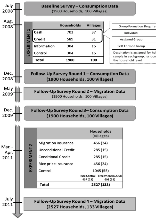
households during the pre-monga season in July 2008. Our analysis will draw on additional rounds of follow-up surveys conducted in December 2008, May 2009, December 2009 and July 2011.
In August 2008 we randomly allocated the 100 villages into four groups: Cash, Credit, Information and Control. These treatments were subsequently implemented in collaboration with PKSF 9 through their partner NGOs with substantial field presence in the two districts. The partner
NGOs were already implementing micro-credit programs in each of the 100 sample villages. The NGOs implemented the interventions in late August 2008 for the Monga season starting in September. 16 of the 100 study villages (consisting of 304 sample households) were randomly assigned to form a control group. A further 16 villages (consisting of another 304 sample households) were placed in a job information only treatment. These households were given
information on types of jobs available in four pre-selected destinations, the likelihood of getting such a job and approximate wages associated with each type of job and destination (see Appendix 1 for details). 703 households in 37 randomly selected villages were offered cash of 600 Taka
(~US$8.50) at the origin conditional on migration, and an additional bonus of 200 Taka (~US$3) if the migrant reported to us at the destination during a specified time period. We also provided exactly the same information about jobs and wages to this group as in the information-only
treatment. 600 Taka covers a little more than the average round-trip cost of safe travel from the two origin districts to the four nearby towns for which we provided job information. We monitored
8 71% of the census households owned less than 50 decimals of land, and 63% responded affirmatively to the question about missing
meals. Overall, 56% satisfied both criteria, and our sample is therefore representative of the poorer 56% of the rural population in the two districts.
9 PKSF (Palli Karma Sahayak Foundation) is an apex micro-credit funding and capacity building organizations in
Bangladesh. It is a not-for-profit set up by the Government of Bangladesh in 1990 .
11
migration behavior carefully and strictly imposed the migration conditionality, so that the 600 Taka intervention was practically equivalent to providing a bus ticket.10
The 589 households in the final set of 31 villages were offered the same information and the same Tk 600 + Tk 200 incentive to migrate, but in the form of a zero-interest loan to be paid back at the end of the monga season. The loan was offered by our partner micro-credit NGOs that have a history of lending money in these villages. There is an implicit understanding of limited liability on these loans since we are lending to the extremely poor during a period of financial hardship. As discussed below, ultimately 80% of households were able to repay the loan.
Table 1 shows that there was pre-treatment balance across the randomly assigned groups in terms of the variables that we will use as outcomes in the analysis to follow. A Bonferroni multiple comparison correction for 27 independent tests requires a significance threshold of α=0.0019 for each test to recover an overall significance level of α=0.05. Using this criterion, no differences at baseline are statistically meaningful.
In the 68 villages where we provided monetary incentives for people to seasonally out-migrate (37 cash + 31 credit villages), we sometimes randomly assigned additional conditionalities to subsets of households within the village. A trial profile in Figure 2 provides details. Some
households were required to migrate in groups, and some were required to migrate to a specific destination. We will not directly analyze the effects of such conditionalities in this paper, but these conditionalities created random within-village variation, which make it possible to study spillover and learning effects from one person to another using instrumental variables.
10 The strict imposition of the migration conditionality implied that some households had to return the 600 Taka if they did not
migrate after accepting the cash. We could not provide an actual bus ticket (rather than cash to buy it) for practical reasons: if that specific bus crashed, then that would have reflected poorly on the NGOs. Our data show that households found cheaper ways to travel to the destination: the average roundtrip travel cost was reported to be 450 Taka. The 150 Taka saving can cover about 5 days of food expenditure for one person at the origin.
12
4. Program Take-up and the Effects of Seasonal Migration
In this section we report results on take-up of the treatment, the effects of seasonal
migration on household consumption at the origin, and on income and savings of the migrant at the destination, and the propensity to re-migrate in 2009 and in 2011 after incentives are removed.
4.1 Migration and Re-migration
Table 2 reports the take-up of the program across the four groups labeled cash, credit, information and control. We have 2008 migration data from two follow-up surveys, one conducted immediately after the monga ended (in December 2008), and another in May 2009. The second follow-up was helpful for cross-checking the first migration report11, and for capturing the migration
experiences of those who left and/or returned later. The two sets of reports were highly consistent with each other, and Table 1 shows the more complete migration rates obtained in May 2009.
In Table 2 we define a household as having a seasonal migrant if at least one household member migrated away in search of work between September 2008 and April 2009. This extended definition of the migration window accounts for the possibility that our incentive merely moved forward migration that would have taken place anyway. This window captures all migration during the Aman cropping season and, as a consequence, all the migration associated with Monga.
About a third (35.9%) of households in control villages sent a seasonal migrant. Providing households information about wages and job opportunities at the destination had no effect on the migration rate (the difference in point estimate is 0.0% and is quite tightly estimated). Either
households already had the information that we made available to them, or the information we made available was not useful or credible. With the $8.50 (+$3) cash or credit treatments, the seasonal
11 Since an incentive was involved, we verified migration reports closely using the substantial field presence of our partner NGOs,
by cross-checking migration dates in the two surveys conducted six months apart, by cross-checking responses across households who reported migrating together in a group, and finally, by independently asking neighbors. The analysis (available on request) shows a high degree of accuracy in the cross reports and, importantly, that the accuracy of the cross reporting was not different in incentivized villages.
13
migration rate jumps to 59.0% and 56.8% respectively. In other words, incentives induced about 22% of the sample households to send a migrant.12 The migration response to the cash and credit
incentives are statistically significant relative to control or information, but there is no statistical difference between providing cash and providing credit.13 Since households appear to react very
similarly to either incentive, we combine the impact of these two treatments for expositional simplicity (and call it “incentive”) for much of our analysis, and compare it against the combined information and control groups (labeled “non-incentive”).
The lower panel of table 2 compares re-migration rates in subsequent years across the incentive and non-incentive groups. We conducted follow-up surveys in December 2009 and in July 2011 and asked about migration behavior in the preceding lean seasons, but we did not repeat any of the treatments in the villages used for the comparisons in the top half of table 2. Strikingly, the migration rate in 2009 was 10 percentage points higher in treatment villages, and this is after the incentives were removed. Regressions of the re-migration choice (discussed in detail in section 6) shows that if a particular household was induced to migrate in 2008, that roughly doubles the chance (a 45 percentage point effect) that it will send a migrant again in 2009. The July 2011 survey focused on migration during the other (lesser) lean season that coincides with the pre-harvest period for the second (lesser) rice harvest. Even two and a half years later, without any further program or
incentive, the migration rate remains 8% higher in the villages randomly assigned to the cash or credit treatment in 2008.
We learn two important things from this migration behavior. First, the propensity to re-migrate absent further inducements serves as a revealed preference based indication that the net benefits from migration were positive for many, and/or that migrants developed some asset during
12 The migrant is almost always male (97%), and often the household head (84% in treatment villages and 76% in control), who is the
only migrant from that household (93%). Migrants make 1.73 trips on average during the season, which implies that migrants often travel multiple times within the season. The first trip lasts 42 (56) days for treatment (control) group migrants. They return home with remittance and to rest, and travel again for 40 (40) days or less on any subsequent trips.
14
the initial experience that makes future migration a positive expected return activity.14 Second, the
persistence of re-migration from 2009 to 2011 (without much further decay after the four potential migration seasons in between) suggests that households learnt something valuable or grew some real asset from the initial migration experience. This persistence makes it unlikely that some households simply got lucky one year, and then it took them several tries to determine (again) that they are actually better off not migrating. It also reduces the likelihood that our results are driven by a particularly good migration year in 2008.
78% of all 2011 migrants provided incentives in 2008 report going back to work for the same employer, which further bolsters our interpretation that the migrants who were induced gained something real and valuable: a connection to an employer. A likely source of uncertainty in the returns to migration thus appears to be the (potential) employer’s incomplete information about the characteristics of specific migrants – are they reliable, honest, hard-working? This would make it difficult for migrants to “learn” from other villagers to resolve the uncertainty, and could explain the null effect of our information treatment. The fact that learning seems to be individual-specific also provides a possible explanation for the fact that some but not all village members migrate. If villagers could learn from the group we would expect to see complete learning overtime driven by the experiences of early adopters (Foster & Rosenzweig, 1995).
We also find that migrants in the incentive treatments (provided cash or credit in 2008) who continue working for the same employer in 2011 are significantly more likely to have formed a connection to that specific employer in 2008, when they were originally induced to go. Specifically, treatment group migrants are 20% more likely to report forming the job connection to their current
14 While we will examine the effect of migration on specific economic outcomes measured in the survey, any one of those outcomes
will necessarily be incomplete, since it is not possible to combine the social, psychological and economic effects of migration in one comprehensive welfare measure. The revealed re-migration preference is therefore a useful complement to other economic outcomes that we use in the analysis below.
15
(2011) employer in 2008 instead of 2007, relative to “regular” migrants in the control group.15 This
is again strongly suggestive that the migrants who were induced to migrate by our treatments formed an asset (a connection to an employer) at the destination, which continued to provide value three years later.
4.2 Effects of Migration on Consumption at the Origin
We now study the effects of migration on consumption expenditures amongst remaining household members during the monga season. Consumption is a broad and useful measure of the benefits of migration, aggregating as it does the impact of migrating on the whole family (Deaton, 1997), and takes into account the monetary costs of investing (although it neglects non-pecuniary costs). Consumption can be comparably measured for migrant and non-migrant families alike, and it helps overcome the problems associated with measuring the full costs and benefits of technology adoption that are highlighted in Foster and Rosenzweig (2010). Our consumption data are detailed and comprehensive: we collect expenditures on 318 different food (255) and non-food (63) items (mostly over a week recall, and some less-frequently-purchased items over bi-weekly or monthly recall), and aggregate up to create measures of food and non-food expenditures and caloric intake.
The effects on expenditures are calculated from a regression where the choice to migrate is instrumented with whether or not a household was randomly placed in the incentive group. In particular we estimate the equation:
Yivj=α+ β Migrantivj + θXivj + φj + υivj
where Yij is per capita consumption expenditure for household i in village v in sub-district j in 2008;
Migrantivj is a binary variable equal to 1 if at least one member of household migrated during Monga
15 The estimating equation is: , , where is a binary variable equal to 1 if
introduced to the employer in 2008 and equal to 0 if introduced in 2007; , is a binary variable equal to 1 if randomly
assigned to receive cash or credit in 2008 and 0 otherwise. P-value for the “sharp” difference test (2008 introduction rather than 2007): 0.09. P-value for the difference test (2008 or 2009 introduction rather than 2007/2006): 0.06. P-value for the difference-in-differences test (2008 vs. 2007, treatment relative to control): 0.26.
16
in 2008 and 0 otherwise; Xivj is a vector of baseline-level controls for household characteristics,
including households income and proxy for assets,φj are fixed effects for sub-districts, and υij is a
mean-zero error term. Migrant is likely an endogenous variable, and we produce consistent estimates of by instrumenting with the experimental treatments. The first stage equation is:
Migrantivj = λ+ ρ Zv+ Xivj +φj+εivj
where the set of instruments Zv includes indicators for the random assignment at the village level
into one of the treatment (cash or credit) or control groups. As is well known, estimates produced in this way show the effect of migration on those households that were induced to migrate by our intervention (that is the local average treatment effect or LATE). In our context this is the most policy relevant parameter: it is the consumption impact of migration on those that are induced to migrate by a policy that incentivizes migration. The LATE is also the average effect of migration on consumption for a well-defined subset of the population.
First stage results in table 3 verify that the random assignments to cash or credit treatments are powerful predictors of the decision to migrate. The second-stage estimates in table 4 show that migration of a household member during the monga season has substantial impact on the remaining household members’ well-being. In all cases the left hand side variables are household level averages using the set of people reported to be living in the household at the time of the survey as the
denominator. We discuss the appropriate choice of denominator in more detail below.
IV estimates using treatment assignment are always larger than OLS estimates. This likely reflects the fact that rich households at the upper end of our sample income distribution are not very likely to migrate (as we will show in section 6) in our analysis of heterogeneity of take-up). In the IV specification, per capita food, non-food expenditures, and caloric intake among induced migrant households increase by 30% to 35% relative to non-migrant households. We also observe
17
some changes towards higher quality diets as food consumption shifts towards protein, and more specifically towards meat and fish, which are more attractive, “tasty” sources of protein in the Bangladesh context. Among non-food items, we observe increases in child education expenditures among migrant households. There is also an increase in expenditures on clothing and shoes, but that is likely an effect of migrants bringing back gifts for their family members.
In terms of magnitude of effects, monthly consumption expenditures among migrant families increase by about $5 per person, or $20 per household due to induced migration. Our survey only asked about expenditures during the second month of monga, and the modal migrant in our sample had not yet returned from their current migration episode (which includes cases where they may have returned once, but left again). We therefore expect the effects to persist for at least another month, and the total expenditure increase therefore easily exceeds the amount of the treatment ($8.50). Furthermore, if households engage in consumption smoothing, then some benefits may persist even further in the future. In any case, the $8.50 is spent two months prior on transportation costs.
Since the act of migration increases both the independent variable of interest and possibly reduces the denominator of the dependent variable (household size at the time of interview), any measurement error in the date that migrants report returning can bias the coefficient on migration upwards. We address this problem directly by studying the effects of migration in 2008 on
consumption in 2009 (where household size is computed using a totally different survey conducted over a year later). The last column of table 4 shows that 2009 effects are about 60-75% as large as the consumption effects in 2008, but still statistically significant. Migration is associated with a 26% increase in household expenditure which is still substantial. These long-run consumption gains are not necessarily from migrants consuming their 2008 earnings over a long period, but because many of those induced to migrate in 2008 were induced to re-migrate a year later.
18
Since the migration decision is serially correlated, measurement error in 2009 migration dates can also bias our estimates. We therefore conduct a number of other sensitivity checks on the consumption results by varying the definition of household size (the denominator). We
conservatively assume that household members present in the house on the day of the interview were present for the entire prior month to consume the reported expenditures, since this variable is least likely to suffer from measurement error and coding problems. The consumption effects in this specification are about 75-80% as large (e.g. 550 calories per person rather than 713), and statistically significant. The effects are similar when we estimate household size based on an entirely different question in the survey (“who currently lives in the household” as opposed to “who is present on the interview date”). Finally, even if we assume that migrants never left and use household size
constructed from baseline data, migration is estimated to increase consumption by 250 calories per person per day.
We can also consider the impact of migration in 2009 on consumption in 2009. Since 2008 treatments do not predict 2009 migration as strongly (first-stage F-stat <5), we have a weak
instrument problem, and do not emphasize these results. Nevertheless, we find that migration in 2009 increases per-capita expenditures by a statistically significant 775 Taka in 2009 (compared to the 355 Taka effect observed in 2008). The larger effect is related to the fact that a select group of “successful” migrants from 2008 were the ones who chose to re-migrate in 2009 (as we show in section 6), and the effects among compliers in the 2009 IV regression are therefore larger.
4.3 Income and Savings at the Destination
Next we examine the data on migrants’ earnings and savings at the destination to see whether the magnitude of consumption gains we observe at the origin are in line with the amount migrants earn, save and remit. Table 5 shows that migrants earn about $110 (7777 Taka) on average and save about half of that. The average savings plus remittance is about a dollar a day. Remitting
19
money is difficult and migrants carry money back in person, which is partly why we observe multiple migration episodes during the same lean season. Therefore, joint savings plus remittances is the best available indicator of money available for consumption at the origin. The destination data suggest that this amount is about $66 (4600 Taka).
The “regular” migrants in the control group earn more per episode, save and remit more per day relative to migrants in the treatment group. This is understandable, since the migrants we induce are new and relatively inexperienced in this activity. Even though the induced migrants had lower earning potential, they earned $105 on average and saved and remitted more than half of that, which suggests a very high rate of return on the $8.50 incentive.
Table 6 breaks down the number of migration episodes and average earnings by sector and by destination. Dhaka (the largest urban area) is the most popular migration destination, and a large fraction of migrants to Dhaka work in the transport sector (i.e. rickshaw pulling). Many others work for a daily wage, often as unskilled labor at construction sites. At or around other smaller towns that are nearer to Rangpur, many migrants work in agriculture, especially in potato-growing areas that follow a different seasonal crop cycle than in rice-growing Rangpur. Migrants earn the most in Dhaka and at other “non-agricultural destinations”: about 5100 Taka or $71 per migration episode, which translates to $121 per household on average given multiple trips. Those working for daily wages in the non-agricultural sector (e.g. construction sites, brick kilns) earn the most.
It is difficult to infer the income these migrants would have received had they not migrated, since we do not have comparable measures of wages and earnings for non-migrants (who engage in a variety of agricultural, self-employment and entrepreneurial tasks at the origin). Observed migrant earnings at the destination (100 Taka per day on average) do compare favorably to the earnings of the sub-sample of non-migrants with salaried employment at the origin (65 Taka per day) and to the profits of small-business entrepreneurs at the origin (61 Taka per day). This comparison is on the
20
basis of a selected sample of migrants and non-migrants with employment, but it is informative about the source from which the extra consumption among migrant households is derived.
While all our data suggest that the extra consumption at the origin is primarily related to migrant earnings, savings and remittance, it is possible that some intensive margin effects (e.g. a switch towards protein or child expenditures) are realized because the husband is away, and there are intra-household gender differences in spending priorities (Thomas, 1994; Duflo, 2003; G. Miller, 2008). However, the intra-household mechanism is unlikely to explain the overall consumption gain (aggregating across food and non-food expenditures). Another possibility is that the overall caloric requirement increases because the migrant works harder, but that also does not directly explain the consumption gain among household members remaining at the origin.
4.4 Is Migration Risky?
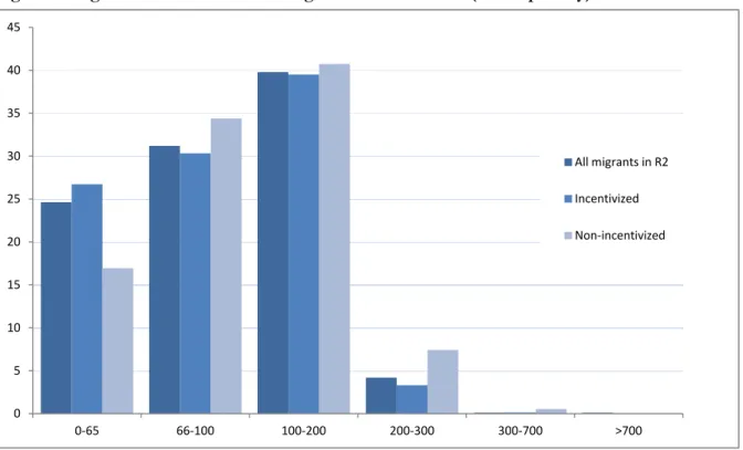
Although migration was profitable on average, and a seemingly sensible strategy for most, there is heterogeneity in the returns to migration. Figure 3 shows that 16% of control group
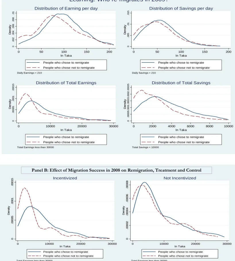
migrants and 27% of migrants from treatment areas earn less than the average earnings for a salaried position at the origin (65 Taka per day). This is admittedly a high bar, since many of the migrants we induced likely would not have been able to secure a steady salaried position at the origin. We asked migrants about their expectations and their actual earnings, and 11% report earning less than they expected. About 80% of households who took a loan to migrate were able to re-pay (there was implicit limited liability on a micro-credit NGOs loan given during a famine). While we cannot accurately measure risk in other (non-economic) dimensions associated with how unpleasant it is for the migrant to stay away from family, the revealed preference (re-migration) data indicates that about half the people induced to migrate the first year choose not to return.
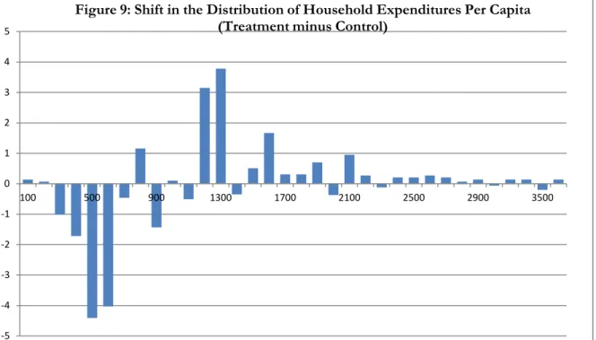
We can examine heterogeneity in the effect of migration on consumption by running “intent to treat” quantile regressions that regresses total expenditures on the cash/credit treatment
21
assignment at different parts of the distribution. This regression shows that the 10th percentile
household in treatment villages experience only a statistically insignificant 14 Taka increase in
expenditures per person, whereas the effect in the top half of the distribution is around 75-115 Taka. The quantile regressions suggest that migration is not valuable for about 10-20% of the population.
In addition to the uncertain returns from migration, the size of the initial investment is not trivial. The travel cost (and the inducement we provided) is equivalent to about 10 days of salaried employment at the origin. The inducement would cover about 25 days of food expenditure for one person during the famine season. Almost always the adult male who is the primary wage earner for the family migrates, and women typically do not work outside the home. In summary, the data suggest that households take a non-trivial risk to travel, and there is about a 10-20% risk of “failure”.
5. A Model of Risky Experimentation
In this section we develop a simple model that is inspired by the three key facts we
documented above: (1) A large number of households were motivated to migrate in response to the 600 Taka incentive, (2) There were positive returns to migration on average, indicating that
households were not migrating despite a positive expected profit, and (3) A large portion of the households that were incentivized to migrate in year one continued to send a seasonal migrant in year two (and again in year 4) and continued to earn a high return to this activity.
Our model is specifically designed to capture the fact that the 600 Taka incentive had a large effect on the migration rate, but is not large in comparison to yearly income variation, nor total income. In particular, the average change in weekly consumption is 307 Taka between rounds 1 and 2 of our survey and 358 Taka between rounds 2 and 3. The standard deviations of these numbers are 635 and 508 Taka respectively. These figures suggest that variation in yearly income dwarfs the size of our 600 Taka payment, a point made forcefully by the observation that weekly expenditures
22
would need to drop just 11 Taka from a base of 860 Taka to save for the bus ticket. Given these observations the challenge for the theory is to explain why 600 Taka can have such an effect on peoples’ choices.
We propose a simple model that is a stripped down version of the classic poverty trap models of Kihlstrom and Laffont (1979) and Banerjee and Newman (1991), and argue that it can explain the three main program evaluation findings. We then use the model to determine additional predictions that should hold in the data. In section 7 we discuss alternative theories that can also generate similar facts and argue that our interpretation is to be preferred on several dimensions.
Consider a household that lives for an infinite number of periods and in each period decides between staying at home and earning a certain income of y and sending a migrant and earning an income of y + b with probability μ(b) and y + g with probability μ (g). We assume that g > b and we also assume that after one migration episode the household becomes informed about whether the return is g or b. The best way to interpret the return in this context is that successful migration (g) requires connections at the destination. Before the first migration episode the household is unsure whether it will be able to find a connection, but once the connection is in place it is permanent.
We assume that the household is a discounted expected utility maximizer with utility function u (that obeys all the usual assumptions), discount factor δand that b and g are such that:
u(y + g) > u(y); and
u(y + b) < u(y).
Given these assumptions, the return to migrating is
Vm= μ g u y+g +μ b 1-δ u y+b +δu y 1-δ
while the return to staying home is
Vh= u y 1-δ .
23
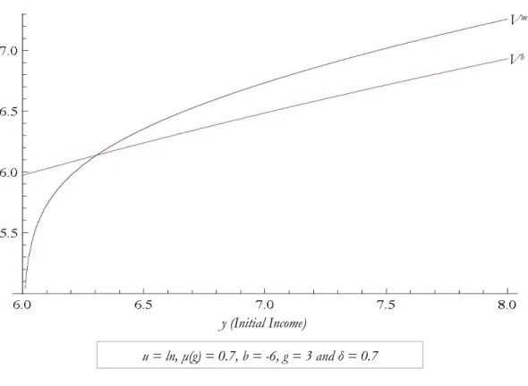
Figure 4 shows a typical plot of Vm and Vh as a function of baseline income y. While the two curves
need not cross, if they do it is usually true that they cross only once with Vm being optimal above
some threshold income y*.16 It is much more likely that the curves will cross like this if the outcome
b is sufficiently bad so that u(y + b) is in the very steep part of the utility function. Figure 4 is drawn under specific parametric assumptions. In particular u is assumed to be the natural logarithm, and in that case the single crossing requires that y + b be close to 0, the point at which the derivative of the log utility function becomes infinite and the utility of consumption infinitely negative. This is a reasonable interpretation of subsistence.
When the conditions for a single crossing are met, the model generates a poverty trap. Households with income y < y* never migrate; they consume their initial income y forever.
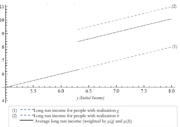
Households that have income of y ≥ y* migrate and learn their migration status. If they are able to find a connection they earn y + g forever after and if they are not able to find a connection they return to consuming y. The long run distribution of income is therefore as depicted in Figure 5. Thus we have a very simple poverty trap, those with initial incomes below a certain level stagnate at that level while those with starting incomes above that point are able to take advantage of migration and push their long run income up by g.
It is well known that this sort of poverty trap requires two things to occur, first, there is a non-convexity in the production technology and second there is a missing market, in that we have shut down borrowing. We believe that both of these assumptions are reasonable in our setting. Migration is clearly a lumpy investment as there is a minimum cost of a bus ticket. Further, despite the influx of micro-credit in this region in recent years, most microcredit organizations require the borrower to spend the money on an entrepreneurial endeavor rather than migration, and
16 The precise conditions for the single crossing can be found in (Banerjee, 2004). Roughly, if y+b is low enough and u is unbounded
below, Vm must lie below Vh in some range. Further, Vm will be above Vh in some range so long as the expected value of migrating
is positive, and u exhibits Decreasing Absolute Risk Aversion (DARA) which implies that the impact of risk aversion becomes negligible at high incomes. Given these conditions DARA is sufficient to ensure that Vmis steeper than Vh and for most common
24
furthermore, require borrowers to remain at the origin to meet the obligations of a frequent
repayment schedule (Shonchoy, 2010; Khandker & Mahmud, forthcoming). We also provide direct evidence that households would like access to credit to migrate by showing that households took up our credit offer, and migrated in response.
Of course, in reality incomes vary across years and those that are close in average income to the cutoff y* will eventually jump from the low-income equilibrium to the high-income equilibrium. Nevertheless, poverty trap models such as this one provide a role for policy in helping those
households whose income is sufficiently low that it is unlikely that they will move between the equilibria. Further, if the return g is large enough, a policy that helps households make the transition can lead to a modest transformation in people’s lives.
5.1 Predictions on the Effects of Different Types of Interventions
We now analyze how external interventions can assist households in making the jump between equilibria. Figure 6 compares three policies. The first panel shows the baseline income threshold y*, identified as the crossing point of the two curves. The second panel shows the new crossing point after a one-off unconditional cash transfer. The third panel shows the crossing point if households are given an incentive similar to our “cash” treatment (of the same size as the transfer in the second panel). The fourth panel shows the impact of an “insurance” program that provides a transfer (again of the same size) only if the household migrates and realizes state b. This fourth panel considers a policy that is similar to a limited liability loan, which is akin to our “credit” treatment.
The figure reveals two testable implications. First, because the poverty trap is driven almost entirely by the possibility of a near subsistence outcome in state b, the limited liability credit
25
(insurance) treatment realizes most of the benefits of the incentive policy.17 The intuition is that if
the poverty trap is driven by income being close to subsistence in the bad state, then removing the possibility of very low consumption removes the lion’s share of the barrier to migration.
Mathematically, the point of intersection of the curves is determined by the implicit equation
u(y+b+x) = 1-μ(b)δ u(y) - μ(g) u(y+g)
with an insurance of size x, and
u(y+b+x)=[1-μ(b)δ] u(y)-μ(g)u(y+g+x)
with an incentive of size x. As discussed above, we require u(y+b) to be small for the poverty trap to exist and as a consequence, adding x to the left hand side of these equations has a large effect. On the other hand, we do not require that u(y+g) be small, in fact it must be relatively large to
compensate for the possible downside of outcome b and ensure a positive expected return. As a consequence, we do not expect the right hand side of the second equation to be changed much by the addition of x. The implication then is that the required change in y* should be similar for an insurance policy or a cash incentive. Empirically, we would predict that our “cash” and “loan” treatments will have a similar size impact on the migration rate.
Second, because the un-conditional transfer increases both Vm and Vh, it has a more limited
impact on y* and migration than an incentive which only increases Vm. This point is obvious, but is
not true in a model in which liquidity constraints are the force that restricts migration. This test is, therefore, an important one because a pure liquidity constraint is probably the most likely alternative explanation for the three facts documented earlier. Under the parametric assumptions used to draw Figure 6, (log utility and specific assumptions about probabilities and investment returns as listed in the figure) an incentive has the same effect on encouraging migration as an unconditional transfer of
17 The insurance policy is also much more cost effective; the incentive must be paid with certainty, while the insurance only pays out
with probability μ(b). To translate this into our practical setting, the loan was repaid in roughly 80% of cases and the total cost of the loan treatment (excluding operating costs) is therefore only 20% of the cost of the incentive treatment.
26
twice the size.18 Since year-to-year variation in income act like un-conditional transfers, this can
explain why our migration incentive scheme induces some households to migrate even when they experience yearly fluctuations in income that exceed the $8.50 incentive.
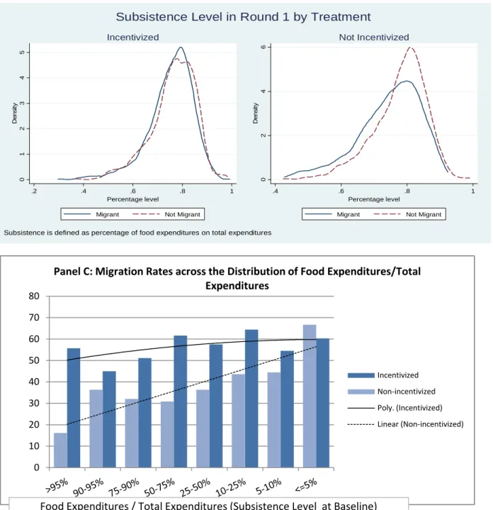
5.2 Predictions on Treatment Heterogeneity: ‘Vulnerability’ and Subsistence
For what types of households do we expect the results above on transfers and incentives to hold? The situation considered in Figure 6 has a particular feature: household income y* is very low. This implies that the transfer policy has a relatively large impact on Vh and therefore that the effect
of the incentive is large relative to the effect of the transfer. This is what is required if we are to match the empirical fact that our incentive has a large effect, but the size of the incentive is small relative to yearly variation in income. If y* is high relative to subsistence then it will no longer be the case that an incentive has a large effect relative to a transfer. Figure 7 illustrates. The left panel shows how a transfer will affect the curves Vm and Vh, while the right panel illustrates the impact of
an incentive. Because income (before considering the effect of the bad outcome) in this example is relatively far from the subsistence point (as illustrated by the fact that Vh is relatively flat) the
transfer has only a small impact on Vh and as a result the incentive and transfer policies have a
similar effect. In such a context it seems unlikely that our incentive would have much of an impact as it is small relative to yearly variation in income and therefore most of the households that are far from subsistence will already have moved to the high income equilibrium. On the other hand, it is easy to see that if income is close to subsistence and Vh is accordingly steeper, then a transfer will
have a much smaller impact on migration rates. This reasoning combined with the fact that the overall impact of our incentive on Vm will be largest when y* is small (due to concavity of the utility
function) leads us to predict that our treatments will have a larger effect on those households that are close to subsistence.
27
5.3 Predictions on Learning
Our model is able to generate such a stark poverty trap because we assume that there is learning about the state of the world after one migration episode. The program evaluation showed that about 50% of households who were induced to migrate in 2008 migrated again in 2009. It would be difficult to generate such a high level of re-migration in a model without learning. We also saw that the majority of households go back to work for the same employer in subsequent years, which suggests that the “learning” is individual-specific, and takes the form of a job connection.
The learning effect generates additional testable implications. First, if we interpret learning as finding out if you can establish a network connection and then keeping that connection, we should see that the incentive has the largest impact on those that do not already have network connections at a destination – this is the group of households that have most to learn. Second, learning should be apparent in the re-migration decision. We should observe households who had a favorable resolution of the uncertainty associated with migration to have higher re-migration propensity, especially in the treatment group. Third, we should see location-specific learning. That is, households that migrate to a particular location (for exogenous reasons) should continue to re-migrate to that location.
Some of the empirical tests implied by the learning assumptions carry an additional benefit in that they help distinguish our model’s predictions from that of the most closely competing
explanation. That alternative model is a simple liquidity constraint (i.e. no money for a bus ticket) preventing migration. In that model, re-migration without the $8.50 incentive in 2009 and 2011 would have to be related to savings from the 2008 migration that gets used for a bus ticket the next year. However, savings from prior period migration operates similarly to an unconditional transfer policy, and as our analysis showed, those savings would have to be very large to generate the same degree of re-migration. Furthermore, location-specific learning and learning from the experiences of
28
others are not necessarily implied by the simple liquidity constraint model, and one would have to add a learning component to that model to get those predictions.
6. Additional Tests of the Model
In summary, our model assumes that households in Rangpur know that there are potentially high returns from migration. They also know that there is a potential downside. Given how close some of them are to subsistence during the Monga season, a failed migration episode would be disastrous. In this situation the incentive we provided is enough to cover a bus ticket plus a little food, and therefore sufficient to rule out the disaster. This enables households to experiment and to discover whether they are able to make an ongoing profit from seasonal migration. If this simple description is correct, then the following additional predictions emerge:
Prediction 1: Cash and Credit treatments should have a similar impact on migration rates;
Prediction 2: The incentive should have a larger effect on households that are close to subsistence;
Prediction 3: The incentive should have a larger impact on households that do not have network connections at the destination;
Prediction 4: Households should exhibit learning in their re-migration choices, including location specific learning;
Prediction 5: Migration should be more responsive to a conditional incentive than an unconditional transfer; and
Prediction 6: Households should be very responsive to an explicit insurance program that covers losses from migration.