ISSN 1440-771X
Australia
Department of Econometrics and Business Statistics
http://www.buseco.monash.edu.au/depts/ebs/pubs/wpapers/
November 2009
Working Paper 14/09
An analytical derivation of the relation between
idiosyncratic volatility and expected stock return
An analytical derivation of the relation between idiosyncratic volatility and expected
stock return
Don U.A. Galagedera*
Abstract
Modelling stock return generating process as a single factor model, we show analytically that the relation between idiosyncratic volatility measured as variance of the residuals and expected stock return in the cross-section may be represented by a parabola that opens to the left and has horizontal axis. This relation is uncovered for stocks of similar volatility and no abnormal return. The sensitivity of the derived relation when these restrictions are relaxed is discussed. Our findings, to a great extent, help uncover the shape of the non-linear inverse relation between idiosyncratic volatility and expected stock return observed in the cross-section in previous empirical studies.
JEL codes: C13, G12
Key words: Idiosyncratic volatility, expected return, analytical derivation , cross-sectional analysis
* Department of Econometrics and Business Statistics, Monash University, 900 Dandenong Road, Caulfield
2 1. Introduction
A number of studies reveal empirical evidence in the cross-section to suggest that idiosyncratic volatility of stocks may have some influence on asset pricing. The evidence however is not consistent. For example, Ang et al (2006), Guo and Savickas (2006) and Frieder and Jiang (2008) report that stocks with high idiosyncratic volatility tend to have very low returns compared to that of stocks with low idiosyncratic volatility. Ang et al (2009) point out that the high idiosyncratic volatility and low return relation is not just a sample-specific or country-specific effect, but it is observed world-wide. Chua, Goh and Zhang (2006) separate idiosyncratic volatility into expected and unexpected idiosyncratic volatility. They use unexpected idiosyncratic volatility to control for unexpected return so that the relationship between expected return and expected idiosyncratic volatility may be observed with more clarity. Chua, Goh and Zhang (2006) find that expected idiosyncratic volatility is positively related to expected return. Jiang and Lee (2005), Malkiel and Xu (2006), Drew, Marsden and Veeraraghavan (2007) and Huang et al (2009) provide evidence that firms that are subject to large idiosyncratic shocks may have high average return. Further evidence of positive association between idiosyncratic volatility and expected return is available in Lintner (1965), Levy (1978), Tinic and West (1986), Merton (1987) and Barberis and Huang (2001). Bollen, Skotnicki and Veeraraghavan (2009) reveal that idiosyncratic volatility is not priced in the Australian market.
The traditional Capital Asset Pricing Model (CAPM) due to Sharpe (1964) suggests that it is the systematic risk that is priced in the market and the unsystematic risk may be diversified away. In this context the relation between idiosyncratic volatility and expected return observed in empirical studies is a puzzle. This relation is observed even when factor models such as the Fama-French (1992) three-factor model and the Carhart (1997) four-factor model known to perform better than the CAPM is used.
Malkiel and Xu (2006) discuss two plausible scenarios as to why idiosyncratic risk may not be completely eliminated through diversification. The basis for one scenario is Merton’s (1987) argument that complexity of rationality of investors may not be captured fully by financial models that assume frictionless markets and complete information. To this end Malkiel and Xu
3
(2006) point out that when one group of investors may not be able to hold the market portfolio due to reasons such as incomplete information, transaction costs and taxes then the rest of the investors may also not be able to hold the market portfolio. This is thought to create an imbalance in the price of stocks thereby investors seeking compensation for idiosyncratic risk. The second scenario stems from the possibility that some investors may not be able to hold the market portfolio notwithstanding the shortcoming that market portfolio is unobservable while others might. In that case a component of the systematic risk may be considered as idiosyncratic risk relative to the theoretically implied market portfolio thereby suggesting that idiosyncratic may be priced. Put simply, market imperfection that may arise due to numerous reasons including heterogeneity in wealth among investors may restrict investors from holding well diversified portfolios. Therefore the investors who do not hold fully diversified portfolios may require a premium for idiosyncratic risk. An account of why idiosyncratic risk may be important is given in Brown and Kapadia (2007) and an investigation of the determinants of idiosyncratic risk is reported in Dennis and Strickland (2004).
The studies that investigate idiosyncratic volatility-expected stock return relation adopt different methods to estimate idiosyncratic volatility. A commonly used measure of idiosyncratic volatility is the standard error estimated in factor models such as the market model, Fama-French three-factor model and Carhart four-factor model. Studies however find that the results are generally robust to the choice of the factor model. Drew, Marsden and Veeraraghavan (2007) consider the difference between total risk and covariance of a stock’s returns with market returns as idiosyncratic volatility. Fama and French (1992) highlight that if systematic risk (beta) of a stock is poorly estimated one should use instead the portfolio beta assigned to individual stocks within the portfolio.1 Following Fama and French (1992), Malkiel and Xu (2006) estimate portfolio residual volatility and assign to individual stocks in the portfolio to obtain idiosyncratic volatility at the stock level.
1 Fitting factor models to a short sample of individual stock returns may induce ‘errors-in-variables’
4
Previous investigations of the relation between idiosyncratic volatility and expected return differ in the study design as well. For example, Ang et al (2006) use daily data and Frieder and Jiang (2008) use monthly data. Many studies estimate idiosyncratic volatility using time series data of one time period and estimate expected return with data of a subsequent time period (Ang et al, 2006 and Frieder and Jiang, 2008). Fu (2009) finds strong evidence that idiosyncratic volatility is time-varying and argues that the negative relationship between expected return and idiosyncratic volatility reported in some studies is questionable as they do not model dynamics of idiosyncratic volatility. Fu (2009) finds a significant positive contemporaneous relation between conditional idiosyncratic volatility estimated in an EGARCH model and expected return. Huang et al (2009) suggest that when investigating the relation between idiosyncratic volatility and expected return the study design should control for immediate prior return. They argue that empirically observed inverse relation between idiosyncratic volatility and expected return may be due to the failure to control for the previous period return. Huang et al (2009) reveal a positive relation between conditional idiosyncratic volatility and expected return and find that the relation remains robust after controlling for return reversal. Jiang, Xu and Yao(2009) highlight that return predictive power of idiosyncratic volatility is induced by its information content about future earnings and once they control for future earning shocks, there is no longer a significantly negative relation between idiosyncratic volatility and future stock returns.
Bali and Cakici (2008) argue that it is difficult to find robustly significant relation between idiosyncratic volatility and expected return due to many issues such as frequency of the data used, weighting scheme used in computing portfolio returns and breakpoints used in the formation of portfolios. Fletcher (2007) highlights that the results in the studies of idiosyncratic risk vary depending on sample period and the model used to estimate idiosyncratic volatility. Wei and Zhang (2005) also express the view that the results in such studies may be driven by data specific to certain sample periods. Bali et al (2005) argue that the significant positive relation between average stock variance (largely idiosyncratic) and the return of the market reported in Goyal and Santa-Clara (2003) is driven by small stocks.
5
Several studies using linear factor models to estimate idiosyncratic volatility reveal a non-linear relation between idiosyncratic volatility and expected return. In this paper we investigate this analytically by assuming a return generating process in the mean-variance framework. That is, we derive the relation between idiosyncratic volatility of a stock and its expected return assuming the market model. Malkiel and Xu (2006) highlight that it is the market factor that captures the most variation in the price of individual securities over time compared to other known factors or proxies. Therefore in our analysis we treat the market model as the base model.2 We reveal analytically that, in the mean-variance framework it is plausible to have an inverse relation between idiosyncratic volatility of a stock and its expected return and this relation may be non-linear. We show that the relation between idiosyncratic volatility estimated as variance in the residuals of the single factor model and expected return of stocks of similar volatility and abnormal return has the shape of a parabola that opens to the left, has horizontal axis and truncated at the vertical axis. While other things being the same, (i) the vertex of the parabola shifts forward and back with increasing and decreasing stock volatility and (ii) the axis of the parabola moves up and down with changing abnormal return. These parabolas demarcate a region where all points associated with idiosyncratic volatility and expected return may lie. When idiosyncratic volatility is estimated as standard deviation in the residuals of the single factor model, the association between idiosyncratic volatility and expected return has the shape of an ellipse which truncated at the vertical axis.
The rest of the paper is organised as follows. The next section presents the derivation of the relation between idiosyncratic volatility and expected return followed by its interpretation in section 3. Section 4 discusses possible extensions of the relation derived in section 2. Section 5 concludes the paper.
2 It is argued that the residuals estimated in the market model may not be considered solely reflecting
idiosyncratic volatility. A reason is that the residuals may be influenced by omitted factors. Later we show that the relation between idiosyncratic volatility and expected return derived here may be extended to multi-factor models as well.
6
2. Derivation of the cross-sectional relation between idiosyncratic volatility and expected
return
We derive a relation between idiosyncratic volatility and expected return assuming the data generating process (DGP) given as
𝑟𝑖𝑡 = 𝛼𝑖+ 𝛽𝑖𝑟𝑚𝑡 + 𝜀𝑖𝑡 (1) where, 𝑟𝑖𝑡is return in stock i in excess of the risk-free rate, 𝑟𝑚𝑡 is the return in the market portfolio in excess of the risk-free rate and 𝜀𝑖𝑡 is an error term independent of 𝑟𝑚𝑡 such that 𝐸 𝜀𝑖𝑡 = 0. The variance of 𝜀𝑖𝑡 is considered as a measure of idiosyncratic volatility and 𝛼𝑖
accounts for abnormal return. 𝛽𝑖 is a measure of systematic risk defined as the ratio of 𝐶𝑜𝑣 𝑟𝑖𝑡, 𝑟𝑚𝑡 and 𝑉𝑎𝑟 𝑟𝑚𝑡 .
Taking the variance of both sides of (1) and re-arranging yields
𝛽𝑖2=𝑉𝑎𝑟 𝑟𝑖𝑡 −𝑉𝑎𝑟 𝜀𝑖𝑡
𝑉𝑎𝑟 𝑟𝑚𝑡 (2)
and taking the mathematical expectation of (1) follows
𝐸 𝑟𝑖𝑡 = 𝛼𝑖+ 𝛽𝑖𝐸 𝑟𝑚𝑡 (3)
Now substituting for beta in (3) from (2) follows
𝐸 𝑟𝑖𝑡 = 𝛼𝑖+ 𝐸 𝑟𝑚𝑡 𝑉𝑎𝑟 𝑟𝑖𝑡 −𝑉𝑎𝑟 𝜀𝑖𝑡
𝑉𝑎𝑟 𝑟𝑚𝑡 (4)
𝐸 𝑟𝑖𝑡 − 𝛼𝑖 2= 𝐸 𝑟𝑚𝑡 2
𝑉𝑎𝑟 𝑟𝑚𝑡 𝑉𝑎𝑟 𝑟𝑖𝑡 − 𝑉𝑎𝑟 𝜀𝑖𝑡 (5)
A sufficient condition for validity of equation (5) is that there exists a linear relation between excess stock return and excess market return.
2.1 Extending the relation to portfolios
In the previous section we derived the relation between idiosyncratic volatility and expected return based on a single-factor model. Here we investigate whether the cross-sectional relation identified at the individual stock level is valid for portfolios as well.
Let us consider a portfolio comprised of n securities with weights 𝑤𝑖 such that 𝑛𝑖=1𝑤𝑖 = 1.
7
𝜀𝑝𝑡 = 𝑟𝑝𝑡 − 𝛼𝑝− 𝛽𝑝𝑟𝑚𝑡 (6)
where 𝑟𝑝𝑡 = 𝑛𝑖=1𝑤𝑖𝑟𝑖𝑡 is the return of the portfolio, 𝜀𝑝𝑡 = 𝑛𝑖=1𝑤𝑖𝜀𝑖𝑡, 𝑉𝑎𝑟 𝜀𝑝𝑡 is the idiosyncratic volatility of the portfolio, 𝛽𝑝 = 𝑛𝑖=1𝑤𝑖𝛽𝑖 is the systematic beta risk of the portfolio
and 𝛼𝑝 = 𝑛𝑖=1𝑤𝑖𝛼𝑖is abnormal return of the portfolio. Now following the same arguments in
section 2 we may obtain the relation between expected return on the portfolio and its idiosyncratic volatility as
𝐸 𝑟𝑝𝑡 − 𝛼𝑝 2= 𝐸 𝑟𝑚𝑡
2
𝑉𝑎𝑟 𝑟𝑚𝑡 𝑉𝑎𝑟 𝑟𝑝𝑡 − 𝑉𝑎𝑟 𝜀𝑝𝑡 (7)
Equation (7) is simply (5) applied to the portfolio and therefore (7) may be interpreted in the same way as we do with (5) in the next section.
3. Interpretation of the relation between idiosyncratic volatility and expected return
In (5) there are four stock specific factors: 𝐸 𝑟𝑖𝑡 , 𝛼𝑖, 𝑉𝑎𝑟 𝑟𝑖𝑡 and 𝑉𝑎𝑟 𝜀𝑖𝑡 . These factors may be considered as variables in the cross-section. Hence to discuss the relation between 𝐸 𝑟𝑖𝑡 and 𝑉𝑎𝑟 𝜀𝑖𝑡 in the cross-section initially we fix the other two variables and later relax those assumptions and explain their influence on the relation between 𝐸 𝑟𝑖𝑡 and 𝑉𝑎𝑟 𝜀𝑖𝑡 . The expression 𝐸 𝑟𝑚𝑡
2
𝑉𝑎𝑟 𝑟𝑚𝑡 is market portfolio specific and therefore for a given market we may treat the
term 𝐸 𝑟𝑚𝑡
2
𝑉𝑎𝑟 𝑟𝑚𝑡 as fixed.
3.1 Case-I: 𝛼𝑖 = 0
Now let us assume that there is no abnormal return so that 𝛼𝑖 = 0. This corresponds to the case
where market model is the true DGP. Then (7) reduces to
𝐸 𝑟𝑖𝑡 2= 𝐸 𝑟𝑚𝑡 2
𝑉𝑎𝑟 𝑟𝑚𝑡 𝑉𝑎𝑟 𝑟𝑖𝑡 − 𝑉𝑎𝑟 𝜀𝑖𝑡 . (8)
Then, for a given market (8) suggests that it is plausible to have an inverse relation between idiosyncratic volatility of a stock and its squared expected return and this association is sensitive to the variation in the stock return.Due to the presence of the variable 𝑉𝑎𝑟 𝑟𝑖𝑡 , equation (8) does
8
idiosyncratic volatility. Therefore we discuss the relation between 𝐸 𝑟𝑖𝑡 2 and 𝑉𝑎𝑟 𝜀𝑖𝑡 given in (8) after controlling for variation in the stock return.3 More specifically, in the mean-variance framework the relation between idiosyncratic volatility and squared expected return in stocks of comparable volatility is negative and linear. This implies that under certain conditions the association between idiosyncratic volatility and expected return may be nonlinear.4
Now we set out to identify the relation between idiosyncratic volatility and expected return as given in (8). For stocks of similar volatility we may assume that 𝑉𝑎𝑟 𝑟𝑖𝑡 is fixed. Then from
(8), for stocks of similar volatility we obtain
𝐸 𝑟𝑖𝑡 2 = 𝐴1− 𝐴2𝑉𝑎𝑟 𝜀𝑖𝑡 (9)
where 𝐴1= 𝐸 𝑟𝑚𝑡
2
𝑉𝑎𝑟 𝑟𝑚𝑡 𝑉𝑎𝑟 𝑟𝑖𝑡 and 𝐴2 =
𝐸 𝑟𝑚𝑡 2
𝑉𝑎𝑟 𝑟𝑚𝑡 which are positive and may be considered fixed.
Consider the equation of two variables x and y given as
𝑦 − 𝑘 2= 4𝑝 𝑥 − 𝑑 (10)
where k, d and p are real numbers and p is non-zero. In the relationship between the variables x and y given in (10), the points (x,y)lie on a parabola with horizontal axis and vertex 𝑑, 𝑘 . If p is positive (negative) the parabola opens to the right (left). Equation (8) has the same structure as (10) such that
𝐸 𝑟𝑖𝑡 − 0 2 = 𝐴2 𝑉𝑎𝑟 𝑟𝑖𝑡 − 𝑉𝑎𝑟 𝜀𝑖𝑡 (11) 𝐸 𝑟𝑖𝑡 − 0 2= −𝐴2 𝑉𝑎𝑟 𝜀𝑖𝑡 − 𝑉𝑎𝑟 𝑟𝑖𝑡 (12)
Hence from (12), for stocks of similar volatility the relation between 𝐸 𝑟𝑖𝑡 and 𝑉𝑎𝑟 𝜀𝑖𝑡 in the
cross-section may be depicted as a parabola that opens to the left with horizontal axis and vertex
3 Interpretation of relationships confining to stocks with specific characteristics is not new. Baker and
Wurgler (2006) in their investigation of investor sentiment and stock returns observe that when beginning-of-period proxies for sentiments are low (high) subsequent returns for small stocks and for stocks with high volatility are high (low).
4 The conditions referred to here are: (i) market model is the true DGP and (ii) stocks have similar volatility
9
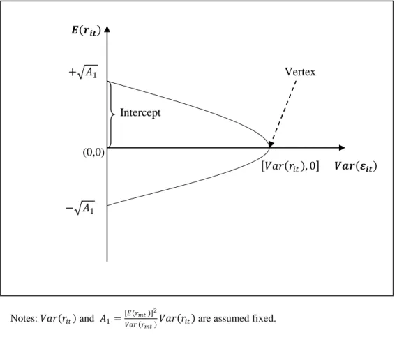
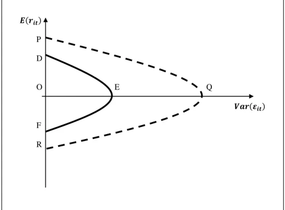
𝑉𝑎𝑟 𝑟𝑖𝑡 , 0 .5 Further, from (9) when 𝑉𝑎𝑟 𝜀𝑖𝑡 = 0 we have 𝐸 𝑟𝑖𝑡 = ± 𝐴1 . The cross-sectional relation between 𝐸 𝑟𝑖𝑡 and 𝑉𝑎𝑟 𝜀𝑖𝑡 identified here is illustrated in Figure 1. Since idiosyncratic volatility is non-negative the parabola is truncated at the vertical axis. Figure 1 reveal that stocks with a given level of idiosyncratic volatility may have high and low expected return. The difference between high and low expected return is higher for stocks with low idiosyncratic volatility than for stocks with high idiosyncratic volatility. The relation between idiosyncratic volatility and expected return for stocks with low volatility and for stocks with high volatility is shown in Figure 2. In Figure 2, the curve DEF (PQR) presents the relation for stocks with low (high) volatility. The intercept associated with the first quadrant in Figure 2 is given by
𝐴1 and is higher for stocks with high volatility than for stocks with low volatility.
3.2 Case-II: 𝛼𝑖 ≠ 0
In this case (16) may be augmented with 𝛼𝑖 as
𝐸 𝑟𝑖𝑡 − 𝛼𝑖 2= −𝐴2 𝑉𝑎𝑟 𝜀𝑖𝑡 − 𝑉𝑎𝑟 𝑟𝑖𝑡 (13)
Equation (13) can be interpreted in the same way as (12) provided 𝛼𝑖 in addition to 𝑉𝑎𝑟 𝑟𝑖𝑡 is considered fixed. Then the vertex of the parabola depicted in (13) lies at 𝑉𝑎𝑟 𝑟𝑖𝑡 , 𝛼𝑖 . An
implication of this is that the curve depicted in Figure 1 now will shift up or down depending on the sign of 𝛼𝑖. The level of shift of course depends on the magnitude of abnormal return estimated
in 𝛼𝑖. An alternative interpretation of this is that, other things being the same, 𝛼𝑖 influences the magnitude of expected return in such a way that (i) when 𝛼𝑖 > 0 the expected return may be
higher than when 𝛼𝑖 = 0 and (ii) when 𝛼𝑖 < 0 the expected return may be lower than when 𝛼𝑖= 0. This is illustrated graphically in Figure 3.
Recall that, a sufficient condition for validity of the above interpretation is a linear relationship between excess stock return and excess market return. Empirical evidence however
5 Equation (11) reveals further, that for stocks of similar idiosyncratic volatility the relation between 𝐸 𝑟
𝑖𝑡
and 𝑉𝑎𝑟 𝑟𝑖𝑡 in the cross-section may be depicted as a parabola that opens to the right with horizontal axis
10
suggests that the market model is not a satisfactory asset price generating process. Further, empirical investigations of the relation between idiosyncratic volatility and expected return generally do so in portfolios. So pertinent questions that arise are whether the relationship between idiosyncratic volatility and expected return uncovered through the single-factor model is valid in the case of DGPs specified by multi-factor models and whether the relationship uncovered at the individual stock level is valid for portfolios. We discuss these issues in section 4. Overall, when the market model is assumed as the true DGP the relation between idiosyncratic volatility in stocks of comparable volatility and no abnormal return (or comparable abnormal return) and expected return has the shape of a parabola that opens to the left and has horizontal axis. All else being the same, (i) the vertex of the parabola moves forwards and backwards with increasing and decreasing stock volatility and (ii) the axis of the parabola moves up and down with varying abnormal return. These parabolas form a region where all points corresponding to idiosyncratic volatility and its associated expected return may lie. We refer to this region as the idiosyncratic volatility-expected return feasible region. Empirical studies investigate the relation between idiosyncratic volatility and expected return under different scenarios. This may cause the points corresponding to idiosyncratic volatility and expected return to be observed in a specific segment of the feasible region as illustrated in Figure 4. This explains why empirical studies may observe mixed results.6 The shaded areas in Figure 4 give examples of segments in the feasible region where empirical observations may be made.
4. Extending the relation to idiosyncratic volatility estimated as standard deviation of the
residuals in the single factor model
In the above analysis we consider variance in the error estimated in the factor model as a proxy for idiosyncratic volatility. Here we derive the relation between idiosyncratic volatility and
6
In empirical investigations there is a possibility of observing a (i) non-linear positive or negative relation, (ii) linear positive or negative relation or (iii) no relation between idiosyncratic volatility and expected return.
11
expected return when idiosyncratic volatility is considered as the standard deviation of the residuals 𝑆𝐷 𝜀𝑖𝑡 estimated in the factor model.
From (5) we have that
𝐸 𝑟𝑖𝑡 − 𝛼𝑖 2 𝑉𝑎𝑟 𝑟𝑚𝑡
𝐸 𝑟𝑚𝑡 2 = 𝑉𝑎𝑟 𝑟𝑖𝑡 − 𝑉𝑎𝑟 𝜀𝑖𝑡 (14)
Now re-arranging the terms in (12) and dividing by 𝑉𝑎𝑟 𝑟𝑖𝑡 follows 𝐸 𝑟𝑖𝑡 −𝛼𝑖2 𝑉𝑎𝑟 𝑟𝑖𝑡 𝑉𝑎𝑟 𝑟𝑚𝑡 𝐸 𝑟𝑚𝑡 2+ 𝑉𝑎𝑟 𝜀𝑖𝑡 𝑉𝑎𝑟 𝑟𝑖𝑡 = 1 (15)
Then substituting 𝐴1 for 𝐸 𝑟𝑚𝑡
2
𝑉𝑎𝑟 𝑟𝑚𝑡 𝑉𝑎𝑟 𝑟𝑖𝑡 and 𝑆𝐷 𝜀𝑖𝑡 for 𝑉𝑎𝑟 𝜀𝑖𝑡 in (13) we obtain
𝐸 𝑟𝑖𝑡 −𝛼𝑖 2
𝐴12
+ 𝑆𝐷 𝜀𝑖𝑡 −0 2
𝑉𝑎𝑟 𝑟𝑖𝑡
2 = 1 (16)
Equation (14) has the form
𝑦−𝑘 2
𝑏2 +
𝑥−ℎ 2
𝑎2 = 1 (17)
where k, h, a and b are real numbers and a and b are positive. In the relationship between the variables x and y given in (17), the points (x,y)lie on an ellipse with center (h,k). If b>a (b<a), the ellipse will have vertical (horizontal) major axis of length 2a (2b). Equation (16) has the same structure as (17). Therefore, for stocks of similar volatility and abnormal return (ie assuming
𝑉𝑎𝑟 𝑟𝑖𝑡 and 𝛼𝑖 are fixed) we may interpret the relation between 𝐸 𝑟𝑖𝑡 and 𝑆𝐷 𝜀𝑖𝑡 as an ellipse
with center (0, 𝛼𝑖), vertices on the vertical axis at 𝛼𝑖± 𝐴1 and the right-hand-side vertex on the
horizontal axis at ( 𝑉𝑎𝑟 𝑟𝑖𝑡 , 𝛼𝑖).7 This is illustrated in Figure 5 for 𝛼𝑖 > 0. Since 𝑆𝐷 𝜀𝑖𝑡 is
non-negative the curve shown there is truncated at the vertical axis.
The curve depicted in Figure 5 moves up and down with changing 𝛼𝑖 and shifts to the left and right with changing 𝑉𝑎𝑟 𝑟𝑖𝑡 demarcating an idiosyncratic volatility-expected return
feasible region. Here too it is clear that, in empirical studies it is plausible to observe a non-linear inverse relation between expected return and standard deviation of the residuals estimated in the factor model. Moreover, for given 𝑉𝑎𝑟 𝑟𝑖𝑡 and 𝛼𝑖 the curve shown in Figure 5 is steeper than the
7 The ellipse will have vertical (horizontal) major axis when 𝐸 𝑟
12
curve in Figure 3. This is because the points on the curve in Figure 5 are the points on the dashed curve in Figure 3 shifted to the left.
As explained in section 2.1, the relationships illustrated in Figures 1-5 are valid for portfolios as well.
5. Concluding remarks
Empirical studies that investigate the association between idiosyncratic volatility and expected stock return report mixed results. For example, there is empirical evidence in the cross-section of a positive, negative and inverse non-linear association between idiosyncratic volatility and expected stock return. It appears that these mixed results may largely be attributed to variation in the study design.
Assuming a linear relation between excess stock return and excess market return, we derive analytically that the relation between idiosyncratic volatility and expected return of stocks of similar volatility and abnormal return may be approximated by a parabola whose axis is horizontal and opens to the left. This finding, to a great extent, helps (i) to explain the inverse relation between idiosyncratic volatility and expected return and (ii) identify the pattern of the non-linear inverse relation between idiosyncratic volatility and expected return that some studies observe in the cross-section. To identify the pattern of association between idiosyncratic risk estimated via a single factor model and expected stock return at individual stock level and at the disaggregated level in the case of portfolios, the study design should simultaneously control for total risk and abnormal return. Studies usually control in one dimension such as for size, total risk and liquidity. We do not refute the findings of previous studies. We provide a framework that may help explain their findings.
13 References
Ang, A., R.J. Hodrick, Y. Xing and X. Zhang (2006) The cross-section of volatility and expected returns, Journal of Finance, 61(1), 259-299.
Ang, A., R.J. Hodrick, Y. Xing and X. Zhang (2009) High idiosyncratic volatility and low returns: international and further U.S. evidence, Journal of Financial Economics, 91, 1-23.
Bali, T.G. and N. Cakici (2008) Idiosyncratic volatility and the cross section of expected returns, Journal of Financial and Quantitative Analysis, 43, 29-58.
Bali, T.G., N. Cakici, X. Yan and Z. Zhang (2005) Does idiosyncratic risk really matter? The Journal of Finance, LX, 905-929.
Baker, M. and J. Wurgler (2006) Investor sentiment and the cross-section of stock returns, Journal of Finance, 61, 1645-1680.
Barberis, N. and M. Huang (2001) Mental accounting, loss aversion and individual stock returns, Journal of Finance, 56, 1247-1292.
Bollen, B., Skotnicki, A. and M. Veeraraghavan (2009) Idiosyncratic volatility and security returns: Australian evidence, Applied Financial Economics, 19, 1573-1579.
Brown, G. and N. Kapadia (2007) Firm-specific risk and equity market development, Journal of Financial Economics, 84, 358-388.
14
Chua, C.T., Goh, J. and Z. Zhang (2006) Idiosyncratic volatility matters for the cross-section of returns- in more ways than one, Working Paper, Lee Kong Chian School of Business, Singapore Management University, http://www.ccfr.org.cn/cicf2006/cicf2006paper/20060126132108.pdf.
Dennis, P.J. and D. Strickland (2004) The determinants of idiosyncratic volatility, Working Paper, McIntire School of Commerce, University of Virginia.
Drew, M.E., Marsden, A. and M. Veeraraghavan (2007) Does idiosyncratic volatility matter? New Zealand evidence, Review of Pacific Basin Financial Markets and Policies, 10, 289-308.
Fama, E.F. and K. R. French (1992) The cross-section of expected stock returns, Journal of Finance, 47, 427-465.
Fletcher, J. (2007) Can asset pricing models price idiosyncratic risk in U.K. stock returns?, The Financial Review, 42, 507-535.
Frieder, L. and G.J. Jiang (2008) Separating up from down: new evidence on the idiosyncratic volatility-return relation, American Finance Association Meetings, New Orleans. Available at SSRN: http://ssrn.com/abstract=970875.
Fu, F. (2009) Idiosyncratic risk and the cross-section of expected returns, Journal of Financial Economics, 91, 24-37.
Goyal, A. and P. Santa-Clara (2003) Idiosyncratic risk maters!, The Journal of Finance, 58, 975-1007.
Guo, H., and R. Savickas, (2006) idiosyncratic volatility, stock market volatility, and expected stock returns, Journal of Business and Economic Statistics, vol.24, pp43-56.
15
Huang, W., Q. Liu, S.G. Rhee and L. Zhang (2009) Return reversals, idiosyncratic risk and expected returns, Review of Financial Studies, (in press), doi:10.1093/rfs/hhp015.
Jiang, G.J., D. Xu and T. Yao (2009) The information content of idiosyncratic volatility, Journal of Financial and Quantitative Analysis, 44, 1-28.
Jiang, X., and Bong-Soo Lee, (2005) On the dynamic relation between returns and idiosyncratic volatility, Working paper, University of Houston.
Levy, H. (1978) Equilibrium in an imperfect market: a constraint on the number of securities in a portfolio, American Economic Review, 68, 643-658.
Lintner, J. (1965) The valuation of risky assets and the selection of risky investment in stock portfolio and capital budgets, Review of Economics and Statistics,vol.47, pp13-37.
Malkiel, B.G. and Y. Xu (2006) Idiosyncratic risk and security returns, Working Paper, University of Texas at Dallas.
Merton, R.C. (1987) A simple model of capital market equilibrium with incomplete information, Journal of Finance, 42, 483-510.
Sharpe W.F. (1964) Capital asset prices: a theory of market equilibrium under conditions of risk, Journal of Finance, 19, 425-442.
Tinic, S. M., and R.R. West, (1986) Risk, return and equilibrium: a revisit, Journal of Political Economy, vol.94, pp126-147.
16
Wei, S.X. and C. Zhang (2005) Idiosyncratic risk does not matter: A re-examination of the relationship between average returns and average volatilities, Journal of Banking and Finance, 29, 603-621.
17
Figure 1. Relation between idiosyncratic volatility and expected return for stocks with similar volatility and no abnormal return relative to the market model
𝑬 𝒓𝒊𝒕 + 𝐴1 Vertex Intercept (0,0) 𝑉𝑎𝑟 𝑟𝑖𝑡 , 0 𝑽𝒂𝒓 𝜺𝒊𝒕 − 𝐴1 Notes: 𝑉𝑎𝑟 𝑟𝑖𝑡 and 𝐴1= 𝐸 𝑟𝑚𝑡 2
18
Figure 2. Relation between idiosyncratic volatility and expected return for stocks of low and high volatility and no abnormal return relative to the market model
𝑬 𝒓𝒊𝒕 P D O E Q 𝑽𝒂𝒓 𝜺𝒊𝒕 F R
Notes: The curve PQR applies to stocks with high volatility and the curve DEF applies to stocks with low volatility.
19
Figure 3. Relation between idiosyncratic volatility and expected return for stocks of similar volatility and with abnormal return relative to the market model
𝑬 𝒓𝒊𝒕 𝛼𝑖+ 𝐴1 Vertex 𝑉𝑎𝑟 𝑟𝑖𝑡 , 𝛼𝑖 > 0 (0,0) 𝑽𝒂𝒓 𝜺𝒊𝒕 − 𝐴1+ 𝛼𝑖 Vertex 𝑉𝑎𝑟 𝑟𝑖𝑡 , 𝛼𝑖 < 0
Notes: The dotted line is the axis of the parabola.
20
Figure 4. Idiosyncratic volatility-expected return feasible region
𝑬 𝒓𝒊𝒕 Feasible region (0,0) 𝑽𝒂𝒓 𝜺𝒊𝒕
Notes: The shaded areas represent examples of segments in the feasible region where empirical observations may be made.
21
Figure 5. Relation between standard deviation of residuals in the market model and expected return for stocks with similar volatility and abnormal return
relative to the market model
𝑬 𝒓𝒊𝒕 𝛼𝑖+ 𝐴1 Vertex 𝑉𝑎𝑟 𝑟𝑖𝑡 , 𝛼𝑖 > 0 (0, 𝛼𝑖) (0,0) SD 𝜺𝒊𝒕 − 𝐴1+ 𝛼𝑖 Notes: 𝑉𝑎𝑟 𝑟𝑖𝑡 and 𝐴1= 𝐸 𝑟𝑚𝑡 2