Conditional Betas

NBER WORKING PAPER SERIES

CONDITIONAL BETAS

Tano Santos

Pietro Veronesi

Working Paper

10413

http://www.nber.org/papers/w10413

NATIONAL BUREAU OF ECONOMIC RESEARCH

1050 Massachusetts Avenue

Cambridge, MA 02138

April 2004

We thank seminar participants at University of Texas at Austin, NYU, University of Illinois at Urbana-Champaign, McGill, MIT, Columbia University, and the University of Chicago. We also thank John Cochrane, George Constantinides, Lars Hansen, John Heaton, Martin Lettau, Lior Menzly, Toby Moskowitz, Monika Piazzesi, and Jessica Wachter for their comments. We thank Arthur Korteweg for outstanding research assistance. Some of the results in this paper were contained in a previous version entitled “The Time Series of the Cross-Section of Asset Prices.” The views expressed herein are those of the author(s) and not necessarily those of the National Bureau of Economic Research.

©2004 by Tano Santos and Pietro Veronesi. All rights reserved. Short sections of text, not to exceed two paragraphs, may be quoted without explicit permission provided that full credit, including © notice, is given to the source.

Conditional Betas

Tano Santos and Pietro Veronesi

NBER Working Paper No. 10413

April 2004

JEL No. G12

ABSTRACT

Empirical evidence shows that conditional market betas vary substantially over time. Yet, little is

known about the source of this variation, either theoretically or empirically. Within a general

equilibrium model with multiple assets and a time varying aggregate equity premium, we show that

conditional betas depend on (a) the level of the aggregate premium itself; (b) the level of the firm's

expected dividend growth; and (c) the firm's fundamental risk, that is, the one pertaining to the

covariation of the firm's cash-flows with the aggregate economy. Especially when fundamental risk

(c) is strong, the model predicts that market betas should display a large time variation, that their

cross-sectional dispersion should be negatively related to the aggregate premium, and that

investments in physical capital should be positively related to changes in betas. These predictions

find considerable support in the data.

Tano Santos

Graduate School of Business

Columbia University

3022 Broadway, Uris Hall 414

New York, NY 10027

and NBER

[email protected]

Pietro Veronesi

Graduate School of Business

University of Chicago

1101 East 58th Street

Chicago, IL 60637

and NBER

I. INTRODUCTION

A firm’s decision to take on a new investment project depends on whether the discounted value of future payouts from the project exceeds the direct current investment cost. To this day, the standard textbook recommendation is to appeal to the CAPM to compute the cost of equity: The rate used to discount future cash-flows should be proportional to the excess return on the market portfolio, where the proportionality factor is the market beta. The task of estimating the cost of equity though is complicated because there is substantial empirical evidence showing that both the market premium and individual assets’ betas fluctuate over time.1 There are many theoretical explanations for the time series variation in the aggregate premium but the same cannot be said of fluctuations in betas.2 Why and how do betas move? How do they depend on the characteristics of the cash-flows that the firm promises to its investors? How do betas correlate with the aggregate premium? How do they correlate with investments in physical capital?

In this paper we answer these questions within a general equilibrium model where both the aggregate equity premium and the expected dividend growth of individual securities are time varying. We show that conditional betas depend on (a) the level of the aggregate premium itself; (b) the level of the firm’s expected dividend growth; and (c) the firm’s fundamental risk, that is, the one pertaining to the covariation of the firm’s cash-flows with the aggregate economy. This characterization yields novel predictions for the time variation of conditional betas as well as their relation with investments in physical capital. Specifically, when the firm’s cash-flow risk (c) is substantial, the model predicts that conditional betas should display a large time variation, that their cross sectional dispersion is high when the aggregate equity premium is low, and that capital investment growth should be positively related to changes in betas. These predictions are met with considerable support in the data

1

On time-varying betas see Bollerslev, Engle, and Wooldridge (1988), Braun, Nelson, and Sunier (1995), Bodhurta and Mark (1991), Campbell (1987), Chan (1988), Evans (1994), Ferson (1989), Ferson and Harvey (1991, 1993), Fama and French (1997), Harvey (1989), and more recently, Franzoni (2001), Lettau and Ludvigson (2001b), and Lewellen and Nagel (2003). On the fluctuations of market premia, see Ang and Beckaert (2002), Campbell and Shiller (1988), Fama and French (1988,1989), Goyal and Welch (2003), Hodrick (1992), Keim and Stambaugh (1986), Lamont (1998), Lettau and Ludvigson (2001a), Menzly, Santos and Veronesi (2004), and Santos and Veronesi (2003).

2

On time varying equity premium, see Campbell and Cochrane (1999), Barberis, Huang, and Santos (2001), Veronesi (2000) and Santos and Veronesi (2003). On time varying betas, see Berk, Green and Naik (1999) and Gomes, Kogan and Zhang (2003).

To grasp intuitively the results in this paper, consider first an asset that has little cash-flow risk, that is, an asset for which cash-cash-flows have little correlation with the “ups and downs” of the economy, see (c) above. In this case, the risk-return trade-off is only determined by the timing of cash-flows, that is by the duration of the asset. As in the case of fixed income securities, the price of an asset that pays far in the future is more sensitive to fluctuations in the aggregate discount rate than an otherwise identical asset paying relatively more today. Clearly, return volatility due to shocks to the aggregate discount rate is systematic. As a consequence, the asset is riskier and thus its beta is higher the longer its duration.

This intuition though does not hold if the asset has substantial cash-flow risk. Indeed, consider now the case of an asset whose cash-flow growth is highly correlated with the growth rate of the aggregate economy. Furthermore, assume as well that the asset has a low duration, that is, it pays relatively more today than in the future. In this case, the total value of this asset is mainly determined by the current level of cash-flows, rather those in the future. The price of the asset is then mostly driven by cash-flow shocks and the fundamental risk embedded in these cash-flows drives also the risk of the asset. Thus, when cash-flows display substantial fundamental risk, the conditional market beta is higher when the duration is lower. If instead the asset has high duration, current cash-flows matter less and the asset becomes less risky.

These findings highlight a tension between “discount effects” (high risk when the asset has a high duration) and “cash-flow risk effects” (high risk when the asset has low duration.) This tension has deep implications for the behavior of the cross section of risk as a function of fluctuations in the aggregate equity premium. Assume first that cash-flow risk effects are negligible compared to discount effects. Then the cross sectional dispersion of conditional betas moves together with the aggregate equity premium: It is low (high) when the aggregate equity premium is low (high). Intuitively, when the aggregate equity premium is low, individual asset prices are determined by the average growth rate of its cash flows over the long run. Given some mean reversion in expected dividend growth – a necessary condition if no asset is to dominate the economy – this implies that the current level of expected dividend growth is not important in determining prices. In this case, assets’ prices have similar sensitivities to changes in the stochastic discount factor and hence have similar market betas as well. Thus when the equity premium is low so is the dispersion in betas. Instead, when the market premium is high, differences in current expected dividend growth matter more in determining the differences in value of the asset. This results in a wide dispersion of price sensitivity to changes in the stochastic discount factor and hence more dispersed betas.

In contrast if cash-flow risk is a key determinant of the dynamics of conditional betas low discount rates lead to an increase in the dispersion of betas. Assets with high cash-flow risk have a component of their systematic volatility that is rather insensitive to changes in the discount rate. However, since a low aggregate discount rate (i.e. good times) tends to yield a low volatility of the market portfolio itself, the relative risk of the individual asset with high cash-flow risk increases, and therefore so does its beta.

Finally we link the fluctuations in market betas to fluctuations in investment. To do so we propose a simple model of firm investment behavior where the standard textbook NPV rule holds. According to this rule, investments occur whenever market valuations are high, which happens when the aggregate risk premium is low, or when the industry is paying relatively high dividends compared to the future, or both. The relation between investment growth and changes in betas is now clear. If cash flow risk is negligible, a decrease in the aggregate equity premium or an increase in current dividend payouts result in a lower conditional beta, as already discussed. Thus a negative relation between changes in betas and investment growth obtains. Instead, when cash-flow risk dominates the risk return trade-off of the asset, there is a positive relation between changes in betas and investment growth. The reason is that now the beta of a low duration asset increases as the aggregate discount decreases.

These observations produce simple empirical tests to gauge the size of discount effects relative to cash-flow effects in determining the dynamics of conditional betas. Empirically, we find that the dispersion of industry conditional betas is high when the market price dividend ratio is high, which in turn occurs when the aggregate market premium is low (e.g. Campbell and Shiller (1989)), confirming that cross sectional differences in cash-flow risk must be large. Similarly, we find that investments growth is higher for industries that experienced increases in their market betas, as well as declines in their expected dividend growth, consistently again with the model and the presence of a significant cross sectional differences in cash-flow risk. Monte Carlo simulations of our theoretical model yield the same conclusion: When cash-flow risk is small and only discount effects matter, the model-implied conditional betas show little variation over time, unlike what is observed in the data. In contrast, when we allow for substantial cash-flow risk our simulations produce fluctuations in conditional betas and investment growth that match well their empirical counterparts.

We obtain our results within the convenient general equilibrium model of Menzly, Santos and Veronesi (2004) – henceforth MSV. This paper, however, differs substantially from MSV, which focused exclusively on the time series predictability of dividend growth and stock returns

for both the market and individual portfolios. The present paper is instead concerned with the equilibrium dynamic properties of the conditional risk embedded in individual securities, a key variable for the computation of the cost of equity and thus for the decisions to raise capital for new investments. As discussed, we fully characterize conditional betas as a function of fundamentals and the aggregate market premium, and obtain numerous novel predictions about their dynamics and their relation to investments in physical capital. This paper is also related to Campbell and Mei (1993), Vuolteenaho (2002), and Campbell and Vuolteenaho (2002), who also investigate the relative importance of shocks to cash flows and shocks to the aggregate discount in determining the cross-section of stock returns and market betas. These papers though focus on unconditional betas while we emphasize the dynamic aspect of betas. This paper relates as well to the recent literature on the ability of the conditional CAPM to address the asset pricing puzzles in the cross section.3 Typically, researchers assume ad-hoc formulations of betas and, in addition, little effort is taken to quantify the magnitude of the variation in betas needed to resolve the puzzles.4 In contrast, in this paper we obtain the market betas within an equilibrium model that successfully reproduces the variation of the aggregate risk premium, as well as the variation in expected dividend growth of individual assets. Our characterization of betas allows us to quantify the magnitude of their variation at the industry level and yields several interesting insights about expected returns: For instance, it is not surprising that industry portfolios have little differences in unconditional expected returns, notwithstanding large differences in conditional betas. In fact, consistently with the model, our empirical results show that the dispersion of betas is high when the aggregate equity premium is low, and viceversa, which imply a little dispersion in expected returns in average. The paper develops as follows. Section II contains a brief summary of the MSV model. Section III contains the theoretical results. In Section IV we propose a simple model of invest-ment and link the fluctuations in betas to changes in investinvest-ments. Section V offers empirical tests as well as simulations of the many implications of the model. Section VI concludes. All proofs are contained in the Appendix.

3

See e.g. Jagannathan and Wang (1996), Lettau and Ludvigson (2001b), Santos and Veronesi (2001), Fran-zoni (2001).

4

II. THE MODEL II.A Preferences

There is a representative investor who maximizes

E _∞ 0 u(Ct, Xt, t)dt =E _∞ 0 e −ρt_{log (C} t−Xt)dt , (1)

where X_t denotes an external habit level and ρ denotes the subjective discount rate.5 In this framework, as advanced by Campbell and Cochrane (1999), the fundamental state vari-able driving the attitudes towards risk is the surplus consumption ratio, St = (Ct−Xt)/Ct.

Movements of this surplus produce fluctuations of the local curvature of the utility function,

Y_t=−uCC u_C Ct= 1 S_t = C_t C_t−X_t = 1 1− Xt Ct >1, (2)

which translate into the corresponding variation on the prices and returns of financial as-sets. MSV assume that the inverse of the surplus consumption ratio, orinverse surplus for short,Y_t,follows a mean reverting process, perfectly negatively correlated with innovations in consumption growth

dY_t=kY −Y_tdt−α(Y_t−λ) (dc_t−E_t[dc_t]), (3) whereλ≥1 is a lower bound for the inverse surplus, and an upper bound for the surplus itself,

Y > λis the long run mean of the inverse surplus and k is the speed of the mean reversion. Herect = log (Ct) and we assume that it can be well approximated by the process:

dc_t=µ_cdt+σ_cdB1_t, (4)

whereµ_c is the mean consumption growth, possibly time varying,σc>0 is a scalar, andBt1is

a standard Brownian motion. Given (3) and (4) then, we assume that the parameter αin (3) is positive (α >0), so that a negative innovation in consumption growth, for example, results in an increase in the inverse surplus, or, equivalently, a decrease in the surplus level, capturing the intuition that the consumption levelCtmoves further away from a slow moving habitXt.6

5

On habit persistence and asset pricing see Sundaresan (1989), Constantinides (1990), Abel (1990), Ferson and Constantinides (1991), Detemple and Zapatero (1991), Daniel and Marshall (1997), Campbell and Cochrane (1999), Li (2001), and Wachter (2000). These papers though only deal with the time series properties of the market portfolio and have no implications for the risk and return properties of individual securities.

6

MSV show thatα≤α(λ) = (2λ−1) + 2λ(λ−1) is needed in order to ensure thatcovt(dCt, dXt)>0

II.B The cash-flow model

There arenrisky financial assets paying a dividend rate, Di t

n

i=1, in units of a

homoge-neous and perishable consumption good. Agents total income is made up of thesencash-flows, plus other proceeds such as labor income and government transfers. Denoting byD0_t the ag-gregate income flow that is not financial in nature, standard equilibrium restrictions require

Ct= _n

i=0Dit. Define the share of consumption that each asset produces, si_t= D

i t

C_t. (5)

Then MSV assume thatsi_t evolves according to a mean reverting process of the form

dsi_t=φisi−si_tdt+si_tσi(s_t)dB_t, for each i= 1, ..., n. (6) In (6) Bt =

B_t1, ..., B_tN is a N-dimensional row vector of standard Brownian motions, si ∈

[0,1) is the average long-term consumption share, φi is the speed of mean reversion, and σi_(s t) =vi− n j=0 sj_tvj = [σi₁(s_t), σ₂i (s_t),· · ·, σi_N(s_t)] (7)

is aN dimensional row vector of volatilities, withvifori= 0,1,· · ·, na row vector of constants withN ≤n+ 1.7

The share process described in (6) has a number of reasonable properties. First, the functional form of the volatility term (7) arises forany homoskedastic dividend growth model. That is, denoting by δi_t = logDi_t, (7) is consistent with any model of the form, dδi_t =

µi(Dt)dt+vidBt, as it is immediate to verify by applying Ito’s Lemma to the quantity si_t =Di_t/(n_j=0D_tj). Second, the assumption that the sharesi_t is mean reverting ensures that no asset will ever dominate the whole economy, as it appears ex-ante reasonable. Third, under the conditionsn_i=1si <1 andφi>n_j=1sjφj, dividends are positive and total income equals total consumption at all times.

In this framework the relative share, si/si_t, stands as a proxy for the asset’s duration. When the relative share is high (low) the assets pays relatively more (less) as a fraction of total consumption in the future than it does presently and then we say that the asset has a high (low) duration. Clearly, high duration assets are also those that experience high dividend growth. Indeed, an application of Ito’s Lemma toδi_t= logDi_t yields

7

The process for the alternative source of income,s0t,follows immediately from the fact that 1−

n i=1sit.

dδi_t=µi_D(st)dt+σiD(st)dBt, where µi_D(s_t) = µ_c+φi si si t −1 −1 2σ i_(s t)σi(st), (8) σi D(st) = σc+σi(st). (9)

andσc = (σc,0, ...,0).8 Notice that the volatility of the share process,σi(st),is parametrically

indeterminate, that is, adding a constant vector to allvi’s leaves the share processes unaltered. A convenient parametrization is then to rescale the vector of constantsvi’s,for i= 0,1, ..., n

so that

n j=0

sjvj =0. (10)

Finally the model offers a simple characterization of the fundamental measure of an asset’s risk, the covariation of the growth rate of its cash-flows with consumption growth,

cov_tdδi_t, dc_t=σ2_c +θi_CF − n j=0

sj_tθj_CF where θ_CFi =vi₁σ_c. (11) The normalization in (10) implies that the unconditionally Ecov_tdδi_t, dc_t = σ2_c +θi_CF, as n_j=0sjθi_CF = 0. Thus, the parameter θi_CF determines the unconditional cross sectional differences ofcash-flow risks across the various assets.9

III. CONDITIONAL BETAS III.A Preliminaries

In the absence of any frictions the price of asseti is given by:

P_ti =E_{t ∞} t e−ρ(τ−t) u_c(C_τ −X_τ) u_c(C_t−X_t) D_τidτ = Ct Y_tEt _∞ t e−ρ(τ−t)si_τY_τdτ , (12)

whereDi_τ =si_τC_τ. Notice that for the total wealth portfolio, the claim to total consumption,

si_τ = 1 for all τ. In this case a complete characterization of the price and return process is possible and they are given by

P_tT W C_t = Φ T W _(S t) = 1 ρ+k 1 +kY ρ St (13) 8

MSV find substantial empirical support for both the fact that dividends and consumption are cointegrated, and that the relative sharesi_/si

tpredicts future dividend growth, as (8) implies.

9

1 +θiCF/σ

2

c can then be taken to be the unconditional cash-flow beta of asseti, the covariance of dividend

anddRT W t =µT WR (St)dt+σT WR (St)dB1,t, where µT W_R (S_t) = (1 +α(1−λS_t))σT W_R (S_t)σ_c (14) σT W_R (St) = 1 +kY St(1−λSt)α kY St+ρ σc. (15)

Equation (13) shows that price of the total wealth portfolio is increasing in the surplus consumption ratio. Roughly, if the surplus consumption ratio is high the degree of risk aversion is low and thus the high price of the total wealth portfolio. As forµT W_R (S_t) andσT W_R (S_t) they are both decreasing inS_t for high values of S_t, as the intuition would have it. However, they are increasing in S_t for very low values of S_t. The reason is that since S_t ∈ (0,1/λ) , the volatility ofS_t must vanish as S_t → 0. This translates in a lower volatility of returns, and, hence, in a decrease in expected returns as well.10

As for individual securities, assume first that their prices can be written as:

P_ti Di t = Φi S_t,s i si t (16) Equation (16) can be intuitively understood appealing to the traditional Gordon model. Here

S_t is the main variable determining movements in the aggregate discount rate, whereassi/si_t, stands for the dividend growth of asseti, as shown in equation (8). In other words, we expect ΦiS_t, si/si_t to be increasing in bothS_tandsi/si_t. Below we provide closed form solutions for ΦiS_t, si/si_t and confirm these intuitions. However, much can be said about conditional betas without making any additional assumptions once we assume that the price dividend ratio can be written as in (16).

Proposition 1: Let the price function be given by (16). Then, (a) the process for returns is given by dRi_t=µi_R,tdt+σi_1,R,tdB1,t+ n j=2 σi_j,R,tdB_j,t (17) where the loadings to the systematic and idiosyncratic shocks are, respectively,

σi_1,R,tS_t, si_t = σ_c+ ∂P_ti/P_ti ∂St/St σ_S(S_t)σ_c+ ∂P_ti/P_ti ∂si_t/si_t σi₁(s_t) ; (18) σi_j,R,tS_t, si_t = 1 + ∂P_ti/P_ti ∂si_t/si_t σi_j(s_t) ;

and σi₁(s_t) and σi_j(s_t) are given in (7) and σ_S(S_t) = α(1−λS_t) is the time varying component of the volatility of the surplus consumption ratiodS_t/S_t.

10

(b) The CAPM beta with respect to the total wealth portfolio can be written as, βiS_t, si/si_t,s_t= covt dRi_t, dRT W_t var_tdRT W t =βi_DISCS_t, si/si_t+βi_CFS_t, si/si_t,s_t (19) where βi_DISCSt, si/sit = 1 + ∂Pi_/Pi ∂St/St σ_S(S_t) 1 + ∂PT W_/PT W ∂St/St σ_S(S_t) ; (20) βi_CF St, si/sit,st = ∂Pi_/Pi ∂si t/sit θ i CF − _n j=0s j tθjCF 1 + ∂PT W_/PT W ∂St/St σS(St) 1 σ2_c (21)

Consider first part (a) of the proposition. As it intuitively follows from (16), consumption shocks,dB_t1,affect returns through three channels: (i) the impact on the dividend of the asset

D_ti =si_tC_t; (ii) the impact on the surplus consumption ratioS_t, which only loads ondB_t1; and (iii) the impact on the sharesi_t, that is, the relative sharesi/si_t.

Part (b) of Proposition 2 now follows naturally from part (a). The CAPM beta has two components to it. The first one captures the component of the covariance that is driven by shocks to the discount factor, and, logically, we refer to it as the “discount beta.” It depends on the sensitivity of the price of the asset to shocks in the surplus consumption ratio, ∂P_∂Si/Pi

t/St. If this elasticity is higher than that of the total wealth portfolio, ∂PT W_∂S/PT W

t/St , the asset is riskier on this account than the total wealth portfolio and thus it has a higher discount beta.

The second component of the return beta is driven by asset’s cash-flow shocks and for this reason we refer to it as the “cash-flow beta.” It depends on the elasticity of prices to shocks in shares, ∂Pi/Pi

∂si t/sit

. Of course, only the component of the shock that covaries with consumption is relevant for pricing and for this reason the expression for the cash-flow beta includes the covariance of dsi_t/si_t with consumption growth itself:

covt dsi_t/si_t, dct =θi_CF − n j=0 sj_tθj_CF, (22)

where we recall thatθi_CF is the parameter that regulates the unconditional covariance between consumption growth and dividend growth, as defined in (11). This component then is driven by the covariance of the cash-flows of assetiwith consumption, and hence with the stochastic discount factor.11

11

Campbell and Vuolteenaho (2002) refer to the “cash flow beta” as bad beta and the discount beta as “good.” Our terminology is closer to that of Campbell and Mei (1996)

The results in Proposition 1 are generic. They rest on assuming that the price dividend ratio can be written as in (16). We show next that this is indeed the case for the two polar cases where either cash-flow effects or discount effects are assumed away. For the general case we show that equation (16) is a very accurate approximation so that the intuitions built in Proposition 1 remain.

III.B The discount beta

To asses the impact of the variation in the discount factor on the cross section of stock prices and returns, we shut down the cross sectional differences in unconditional cash-flow risk, that is, we setθi_CF = 0 for alli= 1, .., nin (11). The next proposition characterizes prices and betas in this case. Part (a) is shown in MSV, and it is reported for completeness:

Proposition 2. Letθi_CF = 0 for alli= 1, .., n.Then, (a) the price dividend ratio of asset i, is given by P_ti Di t = ΦiSt, si/sit ≡ai₀+ai₁Y kSt si si t +ai+ai₂Y kSt (23) whereai =ρ+k+φi−1, ai₀ =aiφi(ρ+k)−1, ai₁ =ai₀2ρ+k+φi/ρρ+φi and ai 2 =ai ρ+φi−1.

(b) The CAPM beta is given by

βi_DISCS_t, si/si_t= 1 + kY St kY St+ρf(si/sit) σ_S(S_t) 1 + kY St kY St+ρσS(St) , (24)

wheref(·) is such that f <0 and f(1) = 1 and it is given explicitly by equation (37) in the Appendix.

Equation (23) shows that asset i’s price dividend ratio is increasing in both si/si_t and

S_t. This is intuitive: As shown in (8), si/si_t is positively associated with the asset’s dividend growth, whereasS_tis negatively associated with the aggregate discount (see equation (14)).

Part (b) of Proposition 2 characterizes the CAPM beta in the case where there are only discount effects. Since f(1) = 1 andfsi/si_t <0, for any level of the surplus consumption ratio, high duration assets, that is, those withsi/si_t >1, have a βi_DISCS_t, si/si_t >1, while the opposite is true for low duration assets. The reason is that high duration assets deliver dividends in the distant future, and thus their prices are particularly sensitive to changes in

the aggregate discount, which is regulated byS_t. These assets are then riskier than otherwise identical assets with lower duration.

An additional characterization of the CAPM beta is provided in the following corollary:

Corollary 3. Let θi_CF = 0 for all i = 1, .., n. Then, for any given level of si/si_t > (<)1, there exists a S_t∗ such that β_DISCSt, si/sit

is decreasing (increasing) in the surplus consumption ratio,St forSt> St∗.

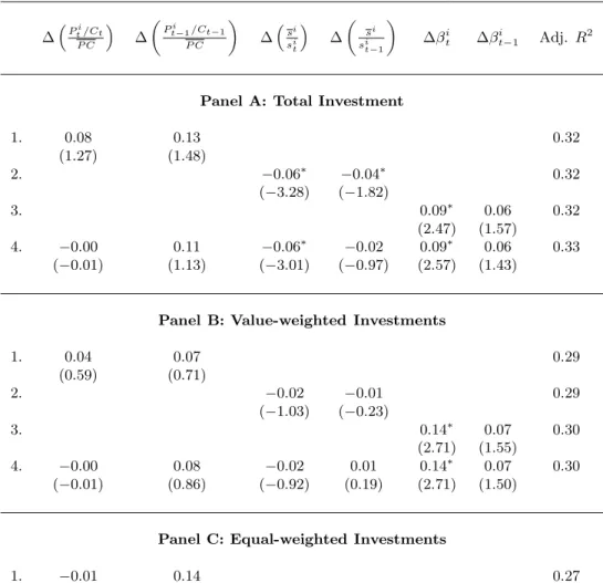
Corollary 3 says that for a given relative sharesi/si_t, the CAPM betas are more dispersed for low, but not too low, levels ofSt.12 To gain some intuition it is useful to turn to Panel A of

Figure 1, where we plot the beta as a function ofSt and si/sit. First, during booms, when St

is high, the aggregate equity premium is low and thus the prices of all assets are mainly driven by the expected dividends in the far future. Mean reversion in expected dividend growth then implies that the variation in the aggregate discount rate has a similar impact on the prices of the different assets, and thus that they all have similar risk: All betas are close to each other and around 1. In contrast, when St is low and the aggregate discount rate is high, agents

discount future dividends considerably, and thus the level of current dividend growth matters more. In this case then, whether the asset has high or low duration is a key determinant of its riskiness and this yields a high cross sectional dispersion of betas when St is low and the

aggregate premium is high.

III.C The cash-flow beta

How do cross sectional differences in unconditional cash-flow risk affect the main conclu-sions obtained in the previous section? In order to obtain sharp implications about cash-flow risk in the context of our cash-flow model (6), we focus in this section on the case with no discount effects, and leave for the next section the more general case. To shut down discount effects, we must ensure that X_t= 0 for all t, and thus we assume α= 0 andY_t=Y =λ= 1.

We then obtain the standard log utility representation with multiple assets. The next propo-sition characterizes the prices and returns of individual securities in this case. Again, part (a) is shown in MSV.

Proposition 4. Letα= 0 and Y_t=Y =λ= 1. Then:

12

Recall that for low levels of the surplus consumption ratio, its volatility has to go down in order to keepSt

above zero. This effect decreases the volatility of the total wealth portfolio. From the stationary density ofSt,

(a) The price dividend ratio of asseti, is given by P_ti Di_t = Φ i_si_/si t ≡ 1 ρ+φi + 1 ρ+φi φi ρ si si_t (25)

(b) The CAPM beta is given by

βi_CF si/si_t,st = 1 + 1 1 + φi ρ si si t  θi_CF − n j=0 sj_tθj_CF   1 σ2_c (26)

Equation (25) shows that, as before, the price dividend ratio is increasing insi/si_t.Part (b) of Proposition 4 provides the CAPM beta with respect to the total wealth portfolio, which is the specialization of the cash-flow beta in equation (21) to this case. In particular, recall that under condition (10),n_j=0sj_tθi_CF ≈0, and thus (26) simply shows that, intuitively, assets with a high unconditional cash-flow riskθi_CF have a high market beta.

Notice that now if θi_CF >0, the premium is higher the lower the relative share, si/si_t, that is the lower the assetsi’s duration. This is also intuitive: assets with lowsi/si_thave prices that are mainly determined by the current flows. Thus, naturally, the covariance of cash-flows with consumption growth, regulated byθi_CF, has substantial impact on the riskiness of the asset. This results in a relatively higher risk for low duration assets. This implication is in stark contrast with the behavior of βi_DISCS_t, si/si_t obtained in the previous section, where we found that high duration assets had a higher risk. As we will see, this implication about the cash-flow beta, βi_CF, carries over in the general case, yielding a tension between discount betas and cash-flow betas.

III.D Betas in the general case

The general model, where the cash-flow and discount effects are combined, is more complex than either one of the cases discussed so far. For this reason, an exact closed form solution for prices and the corresponding CAPM representation is not available. However, there is a very accurate analytical approximate solution of the same form as (16), where the nature of the approximation is contained in the Appendix of MSV. As in equations (23) and (25), we find P_ti/Di_t≈ΦiSt, sit/si = Φi₀(St) + Φi1(St) si si_t (27) where Φi_j(S_t), j = 1,2, are linear functions of S_t given explicitly in (34) and (35), respec-tively. The important additional feature of this pricing formula is that it now depends on the

parameter θi_CF, that is, the parameter defined in equation (11) that regulates the long-term unconditional cash-flow risk. Generically speaking, a high θi_CF tends to decrease the price of the asset.

Given ΦSt, si/sit

in (27), we can apply the general result in Proposition 2 (b), and thus obtain the beta representation (19). The formulas are explicitly given in (36) and (38) in the Appendix. Briefly,βi_DISCSt, si/sit

is essentially identical to the one obtained in equation (24), with the only additional feature that a high unconditional cash-flow riskθi_CF is associated with a higher discount beta.

The most interesting effect of the general model, instead, pertains to the cash-flow beta

βi_CFSt, si/sit,st

.As in the case with no discount effects,βi_CFSt, si/sit,st

is still decreasing in the relative share si/si_t when the unconditional cash-flow risk θi_CF > 0 (see discussion in Section III.C). In addition, however, it now depends also on the surplus consumption ratioSt.

That is, how important cash-flow risk is also depends on the aggregate state of the economy. Panels B and C of Figure 1 plot the βi_CFS_t, si/si_t for the cases where θi_CF > 0 and

θi_CF <0, respectively.13 In contrast to the discount beta βi_DISCS_t, si/si_t, we can see that

βi_CFS_t, si/si_t tends to display a higher relative cross sectional dispersion during good times, that is, whenS_t is high. Intuitively, as we discussed in Proposition 4 (b), a low duration asset with a positive unconditional cash-flow riskθi_CF >0 tends to have a high beta, as its price is mainly determined by current dividends rather than the future ones. This component of the systematic volatility of the asset price is relatively insensitive to the fluctuations in the discount rate, as it stems from cash-flow fluctuations. However, during good times the volatility of the total wealth portfolio is lower than in bad times, as shown in equation (15). Thus, the low duration asset tends to become relatively riskier – compared to the total wealth portfolio – during good times, that is, whenS_t is high. A similar argument holds for θi_CF <0, although in this case the source of the difference stems from the hedging properties of the asset. In this case, we obtain that the cash-flow beta, which is negative, is lower whenS_tis high when assets have low duration. In summary, independently of whetherθi_CF is positive or negative the cross sectional dispersion of cash-flow betas increases when the aggregate premium decreases.

13

We make use of the normalization (10) and thus set Σni=1sitθiCF ≈ 0. The plots are for values of the

parameters of the underlying cash flow process that are of the same magnitude as the ones found in the estimation procedure below for the set of industry portfolios we use.

IV. CONDITIONAL BETAS AND INVESTMENTS

The cost of equity is a key determinant of the firm’s decision to invest. To address the relation between investment decisions and time-varying betas we propose next a simple model of the firm’s investment behavior. In this section, we interpret the n risky assets introduced in Section II as industries, and the betas derived in Section III as industry portfolio betas. We then link the investment decisions of a small firm with its corresponding industry beta, a relation that is taken to the data in the empirical section. MSV indeed show that the cash-flow model (6) offers a reasonable description of the cash-flows associated with industry portfolios.

IV.A A simple model of investment

Consider a small firm in industryi faced with the decision of whether to undertake an investment project at timet. We assume this project can only be undertaken at timet, as it vanishes afterwards, has a fixed scale, and requires an exogenous initial investment amountIt.

We also assume that projects arrive independently of the firm’s previous investment decisions.14 All these assumptions imply that the textbook NPV rule holds and the firm chooses to invest by simply comparing the value of the discounted cash flows to the investment needed to attain them,It.If the investment does take place, the project produces a continuum random cash flow CF_τ up to some random time t+T, whereT is a random variable exponentially distributed with parameterp >0. We assume that the cash flow process is given by

CF_τ =aD_τiε_τ.

whereais a constant. HereD_τi is the aggregate dividend of industryiandετ is an idiosyncratic

component that follows a mean reverting process

dε_t=k_ε(1−ε_t)dt+√ε_tσ_εdB_t,

where dB_t is uncorrelated with the Brownian motions introduced in Section II. This setting ensures that the cash flows produced by the new investment inherits the cash-flow risk char-acteristics of industry i, although the idiosyncratic component may drift these cash flow far away from the industry mean.15

14

Berk, Green, and Naik (1999) and Gomes, Kogan, and Zhang (2003) have recently proposed similar models of investments though to answer different questions.

15_{We do not attempt here to offer a general equilibrium model of investments, as doing so is outside the scope}

The discounted value of the project’s cash-flows, V_t, is now easy to calculate. Assuming that investors are well diversified the value of the project at timetis

Vt=Et _t+T t e−ρ(s−t)uc(Cs−Xs) uc(Ct−Xt) CFsds (28) and investment occurs according to the textbook NPV rule, that is, ifVt> It.

To understand the relation between betas and investments, it is convenient to rewrite (28), the value of the specific project at hand,16 in the more familiar form (see Appendix):

Vt=Et _t+T t e− s t rτ+βτ×µT Wτ dτ_CF sds , (29)

where r_τ is the risk free rate at τ, µT W_τ is the expected excess return on the total wealth portfolio, and β_τ =βS_τ, si/si_τ, ε_τ= Covτ dV_τ/V_τ, dRT W_τ V ar_τdRT W t

is the beta with respect to the total wealth portfolio. Equation (43) in the Appendix shows thatβ_τ has a representation similar to the one in (19).

It is clear now that even when the standard positive NPV rule applies and the conditional CAPM holds, as they do in this simple framework, the prescription of computing separately the cost of capital and expected future cash flows is misleading as

E_t e−tsrτ+βτ×µT Ws dτ_CF s =E_t e−tsrτ+βτ×µT Wτ dτ E_t[CF_s].

Even when the expected excess returns on the market portfolioµT W_s is constant, the presence of predictable components in dividend growth induce time varying betas that naturally cor-relate with the future cash flows of new projects.17 Variation in the aggregate premium only complicates the problem further.

alive at any timetin industryi, anda= 1/N, an application of the central limit theorem shows that the total cash flows from these projects approachesDtiasN → ∞. The model can then potentially be closed by a simple

assumption that the industry produces a total output rate given byKti =Dit+Iti, whereIti is the aggregate

investment defined by the optimal investment rule below.

16

This should not be confused with the value of the firm, which includes the portfolio of current projects plus the options to invest in all future projects that arise.

17

And there are predictable components in dividend growth. MSV show that the relative sharesi/sitforecasts

dividend growth for the majority of industries in our sample (see their Table III.) Ang and Liu (2004) also emphasize that the cost of capital cannot be computed separately from the expected cash-flows in a setting where the beta dynamics are assumed exogenously.

Given that the decision to invest has to be taken before ε_t is known and thatE[ε_t] = 1, the Appendix shows that NPV rule is given by

V_t=aDi_tΦV S_t, si/si_t> I_t (30) where ΦV St, si/sit

is as in (27) but where the parameter ρ is substituted for ρ+p. That is, investments occur when prices are high, which occur when either the surplus consumption ratio St is high, Dti is high or si/sti is high. In our setting, however, Dit = sitCt. From the

formula of ΦV St, si/sit

in (27), and assuming that the size of investment grows with the economy,It=bCt, we find that investment occurs whenever

V_tN = s i t siΦ V 0 (St) + ΦV1 (St)> I∗= b asi, (31)

where V_tN = V_t/C_t, and Φ₀V (S_t) and ΦV₁ (S_t) are as in (34) and (35) in the Appendix with the only exception that ρ is substituted forρ+p,as already mentioned. The implications for the firm’s investment rule are now clear and intuitive. Given that ΦV₀ (S_t) and ΦV₁ (S_t) are positive, increasing functions ofS_t, investments occur when the surplus consumption ratio,S_t,

is high, that is whenever the aggregate premium is low.18 It also occurs wheneversi_t/siis high, that is, when the industry expected dividend growth is low. The reason is that an industry with high dividend today relative to those in the future is one with high valuations as well, as measured for instance by the price consumption ratio.

IV.B Changes in betas and changes in investments

Equation (31) offers a complete characterization of the firm’ investment policy. Our purpose next is to link this behavior to the variation in betas. After all, cross sectional differences in the discount can only arise due to cross sectional differences in betas. Here turning to Figure 1 is helpful to offer intuitive predictions about the relation between investments and betas. The question is whetherβis high when prices are high, or, to put it differently, whether

β increases or decreases when prices increase, since the decision to invest is related to changes in prices that pushV_tN aboveI∗. The classical CAPM setting would intuitively suggest that a high beta implies a high cost of capital, and thus lower prices discouraging the firm to invest. The endogenous time variation in betas offers a more subtle picture of the cross sectional differences in the cost of equity firms may face depending on the industry they belong to.

18

This proposition has, of course, received considerable attention. See, for example, Barro (1990), Lamont (2000), Baker, Stein, and Wurgler (2003), and Porter (2003).

Assume first that there are no cash flow effects (θ_CF = 0) so that β_t=β_DISC(.), which is plotted in the top panel in Figure 1. Equation (31) shows that investment occurs when the surplus consumption ratio St is high or the relative share si/sit is low. As shown in the top

panel of Figure 1, the combination of a highStand a lowsi/sit results in a low discount beta.

Thus, if discount effects dominate the risk-return characteristics of projects, investment occurs when betas decrease.

The opposite conclusion obtains in the presence of substantial cash-flow risk. In this case, the total beta is the sum of the discount beta and the cash flow beta. Consider first the case whereθCF >0 (the middle panel in Figure 1.) The cash-flow beta is high whenever the

surplus consumption ratioStis high or the relative sharesi/sit is low, the conditions that lead

to higher investment according to (31). In addition, a positiveθCF implies that, on average,

an increase in the surplusSt is correlated with an increase in the sharesit and thus negatively

correlated with the relative sharesi/si_t. Thus, on average, the cash-flow beta of assets with a highθ_CF >0 moves along the ray of low surplus−high duration to high surplus−low duration. This implies that ifθ_CF is positive and sufficiently large, a positive relation between investment growth and change in betas should occur.

The case where θ_CF < 0, plotted in the bottom panel of Figure 1, leads to the same conclusion, although the intuition is slightly more involved. First of all, a negativeθ_CF <0 implies on average cash-flow betas move along the ray of low surplus−low duration area to the high surplus−high duration. Moreover β_CF is increasing along this diagonal. Since the effect of changes in S_t on prices is intuitively the most important one – all prices are high in good times – it follows that, on average, a positive relation between investment growth and the cash-flow beta obtains as well.

V. EMPIRICAL ANALYSIS V.A Data

Our data and estimation of parameters can be found in MSV. Briefly, quarterly dividends, returns, market equity and other financial series are obtained from the CRSP database, for the sample period 1946-2001. We use the Shiller (1989) annual data for the period 1927-1945, where we interpolate the consumption data to obtain quarterly quantities. We focus our empirical exercises on a set of twenty value-weighted industry portfolios for which summary statistics are provided in Table AI. There are two reasons to focus on this set of portfolios: The first is that they enable us to obtain relatively smooth cash-flow data that are a-priory consistent with

the underlying model for cash-flows put forward in this paper (equation (6)). We concentrate our analysis on a coarse definition of industries – the first two SIC codes – which are likely to generate cash-flows for a very long time. A second reason to focus on industry portfolios is that, as shown by Fama and French (1997), they display a large time series variation in their betas, precisely the object of interest in this paper.19 Moreover, industry portfolios show little, if any, cross sectional dispersion in average returns. This may suggest that there is little cross sectional dispersion in cash-flow risk across these portfolios. We show how testing whether the cross section of betas is positively or negatively related to the aggregate equity premium uncovers instead important cash-flow effects. This set of test portfolios then seems an ideal laboratory to test many of the implications of the model.

The cash-flow series includes both dividends as well as share repurchases (constructed as in Jagannathan, Stephens, and Weisbach (2000)) a detailed description is included in the Appendix in MSV. With some abuse of terminology we use the expressions “cash-flow” and “dividend” interchangeably throughout the empirical section. Finally consumption is defined as real per capita consumption of non durables plus services, seasonally adjusted and is obtained from the NIPA tables. All nominal quantities are deflated using the personal consumption expenditure deflator, also obtained from NIPA.

MSV contain a number of tests showing that logD_tiand log(C_t) are cointegrated series for most industries (twelve out of twenty), and that indeed the relative share si_t/si_t is the strongest predictor of future dividend growth, as the model implies. Finally, they show that the cross-sectional and time variation in price dividend ratios implied by the model nicely line up with the empirical data.

As for the definition of investments, we define them as Capital Expenditures (Compustat Item 128) over Property, Plants, and Equipment (PPE, Compustat, Item 8). Individual firm investments are aggregated to industry investments in three different ways: Total Capital Expenditure over Total PPE, referred to as Total Investments, or as a value-weighted or equally weighted average of firm investments. Data are available from 1951 - 2001, at the annual frequency.

Finally, Table I reports the estimates of the parameters used for the simulations below.

19

Braun, Nelson, and Sunier (1995, page 1584-5) also find that “the evidence for time-varying betas is some-what strong” for their set of industry and decile portfolios. In addition these authors compare the rolling regression estimate of the five year window beta with the estimate obtained from an EGARCH model and show that these two estimates track each other rather well (see their Figure 1.) Ferson and Harvey (1991) also find substantial variation in the betas of the industry portfolios in their sample.

These parameters are as in MSV and the reader is referred to Appendix B in that paper for details.

Estimation of θi_CF

As repeatedly emphasized, θi_CF is the key parameter in evaluating many of the asset pricing implications of the model. We estimate this parameter using two alternative procedures. Our first estimate relies exclusively on cash-flow data. Specifically we make use of expressions (11) and (10) which yieldθi_CF =Ecov_tdδi_t, dc_t−var(dc_t). Given thatE_t[dc_t] is constant, we simply haveθi_CF = covdδ_ti, dc_t−var(dc_t) and estimate it accordingly. These estimates are reported in Table I in the column denotedθi_CF-Cash-flow.

Our second estimation procedure uses stock return data to back out the cash-flow pa-rameterθi_CF.This estimation procedure is motivated by the fact that, as we show below, when we estimateθi_CF using only cash-flow data, the cash-flow beta βi_CF fluctuates too little. As noted by Campbell and Mei (1993, page 575) cash-flow betas are only imprecisely estimated and thus it is natural to ask whether the lack of variation in betas is due to a downward bias in our estimates ofθi_CF.Specifically, we estimateθi_CF and vi using a GMM procedure where the moment conditions are constructed as follows. First define,

ui_1,t = Ri_t−βiSt, si/sit,st RM_t ui_2,t = Ri_t2−σ2_Ri t S_t, si/si_t,s_t

whereβiS_t, si/si_t,s_t is the theoretical beta as given in expression (19) andσ2 Ri

t

S_t, si/si_t,s_t

is the theoretical variance of returns implied by expression (17). The moment conditions are then given by

Eui_1,t, ui_1,tRM_t , ui_2,t

=0

To make sure that the system is not underidentified we assume, for simplicity, that the vector of constants governing the diffusion component of the share process (see expression (6)) is such that vi = θi_CF σc ,0, . . . ,0, vi,0, . . . ,0 ,

where the only non-zero element besides θi_CF/σ_c, the systematic component, occurs in entry

i+ 1.

The results of the estimation are contained in Table I under the headingθi_CF−Return. As can be readily noted, there is a remarkable difference in the estimates across these two alternative procedures. First notice that the estimates in, absolute terms, are off by a factor of

ten! Estimatingθi_CF using returns emphasizes the point that resorting only to cash-flow data may seriously underestimate the amount of cash-flow risk present in the data. Second, notice as well that many of the estimates flip signs, and whereas negative signs dominate when only cash-flow data is used, positive ones do when returns data is used.

V.B Can the model generate substantial variation in betas?

Fama and French (1997) provide a simple estimator of the time variation in betas: Under the assumption that the sampling error associated with the market betas is uncorrelated with the true value of the beta, the variance of the rolling regression beta is the sum of the variance of the true market beta and the variance of the estimation error, or in symbols,

σ2 β_trolling-regress. =σ2(β_t) +σ2(ε_t), (32)

where β_trolling-regress. is the estimated rolling regression beta, β_t stands for the true beta and

εt is the estimation error.20

Table II reports the estimates forσ2(β_t) for our set of industry portfolios. The average standard deviation of betas is .14, which, incidentally, is only slightly higher than the one obtained by Fama and French (1997) for a set of 48 industry portfolios. Thus if the beta of an average industry were to be one, a two standard deviation of beta yields variation between .74 and 1.28, which is rather substantial. Some of them, like Retail, Petroleum, Mining, Department Stores, Fabrication Metals, and Primary Metals display standard deviation of betas that are above .20. Thus if the average beta of retail is around one, a two standard deviation around the mean yields betas that fluctuate between .46 and 1.54!

Can our model yield comparable variation in betas? The next two columns in Table II report the standard deviation of the betas in our model in 40,000 quarters of artificial data. The column under the heading “θi_CF−Cash-flow” reports the standard deviation of theoretical betas when θi_CF is estimated using only cash-flow data, that is as the covariance of dividend and consumption growth. The variation of betas in this case does not match the one observed in the data and hovers around .02. The only exception is Primary Metals, where the variation of the theoretical beta reaches 0.10.

20

Clearly, when the variance of the true beta is estimated as the difference of the variance of the rolling regression beta and the variance of the estimation error there is no guarantee that the variance of the true beta is greater than zero. In this case we follow Fama and French (1997) and set the variance equal to 0. This occurs in our sample for only two industries, Electrical Equipment and Manufacturing.

The results are rather different when we estimate the cash-flow parameters using returns data, as described in the previous section. These results are reported in the column under the heading “θi_CF−Returns.” In this case the average standard deviation is given by .10, which is close to the average standard deviation obtained through the Fama and French (1997) procedure, see equation (32) above, which was .14. Also notice that in the case ofθi_CF− Cash-flow only one industry out of twenty had a standard deviation of beta above .10, Primary Metals. Now the number has increased up to ten. For instance, the model can generate a substantial variation in the betas of Primary Metals, Utilities and Food, which also had a large variation in the betas as estimated by Fama and French (1997). There are clearly some shortcomings as, for example, Electrical Equipment where the data suggests a very low variation in the market loading whereas the model attributes a standard deviation .22. However, small sample accounts for a large part of these differences. In fact, Figure II reports the results of a different simulation exercise: we obtain 1,000 samples of artificial data, each 54 years long. On each sample we estimate the standard deviation of beta as described in (32). The top panel in Figure II reports the 95% simulation bands of σ(β_t) (solid lines) along with the point estimates in the data (stars) for the case where θi_CF is estimated using cash flows. The bottom panel reports the same quantities for the case whereθi_CF is estimated using stock returns. In this latter case, it is indeed the case that the majority of point estimates ofσ(β_t) from the data (stars) fall in the simulated bands (thirteen out of twenty). Whenθi_CF is instead estimated from cash flow data, the empirical estimate of σ(β_t) fall in the bands for only five industries, a result that is in line with those reported in Table II.

In summary then, the estimate ofθi_CF turns out to have a rather substantial impact on the behavior of the conditional beta, not only the unconditional one, as one may suppose at first. The reason is that the duration effect associated with cash-flow risk, the fact that assets with high cash-flow risk have higher risk the shorter their duration, is a key determinant of risk. But if this is the case, this observation has strong implications for the time series behavior of the cross sectional dispersion of risk over time, to which we now turn.

V.C The cross sectional dispersion of betas

We now investigate the time series properties of the cross sectional dispersion of betas. We run the following time series regressions

Ri_t+1 =αi+βi_{U p} IdxU p_t RM_t+1 +βi_DoIdxDo_t RM_t+1+εi_t+1 whereRi

respectively, andIdxU p_t and IdxDo

t are indicator functions of whether times are good (Up) or

bad (Do), that is, whether the aggregate equity premium is low or high. We consider two different proxies for good and bad times: (i) the market price dividend ratio, withIdxU p_t = 1 if the price dividend ratio of the market is above its historical 70 percentile, and IdxDo_t = 1 if price dividend ratio is below its historical 30 percentile; and (ii) the surplus-consumption ratioSt itself, where againIdxU pt = 1 or IdxDot = 1, if the surplus is above its 70 percentile,

or below its 30 percentile.21 How can we formally test whether the cross sectional variance of βi_{U p} is higher or lower than the cross sectional variance of βi_Do? Assuming that βi_{U p} and

βi_Do are drawn from a normal distribution with two different variances, σ2_{U p} and σ2_Do, we can use the statisticsV arCSβi_{U p}/V arCSβi_Do, which has anF-distribution, with 19 degrees of freedom. The results are in Table III.

Panel A of Table III shows that for both samples, 1927 - 2001 and 1947 - 2001 the dispersion of betas is significantly higher when the aggregate equity premium is low, with the exception of the long sample when the surplus consumption ratio is used a sorting variable, in which case the difference is not statistically significant. In particular, there is no evidence that dispersion of betas is higher during bad times.

These findings have a clear interpretation in light of our model. Essentially, cash-flow effects have to be strong in order to undo the positive relation between the cross sectional dispersion of betas and the aggregate equity premium that discount betas induce (see Corollary 3). That is, these findings can be explained by either a strong time variation in the cross-sectional dispersion of expected dividend growth, proxied by STDCSsi/si_t, and/or substantial unconditional cash-flow riskθi_CF = 0. Indeed, the effect of the time variation insi/si_tcan also be seen in the last line of Panel A, where it shows that the dispersion of betas is higher when also the dispersion of relative shares is high, especially in the postwar period.

To disentangle the effects of the dynamics of the dispersion of relative shares STDCSsi/si_t

from the unconditional cash-flow risk, we decompose in Panel B of Table III the variation in return betas in its two basic sources, variation in aggregate discounts (S_t) and variation in dispersion in cash-flow growth si/si_t. In this case, in addition to Up and Down periods as defined in Panel A, we also define an index of whether the cross sectional dispersion of relative shares STDCSsi/si_t is high or low, where we set the cutoff levels to the median in all cases now in order to have a sufficient number of observations for each of the four categories (Up-Hi,

21

We obtain the surplus consumption ratioSt by computing a sequence of consumption shocks dBt=dct−

Do-Hi, Up-Lo, Do-Lo). As before, we run the time series regressions Ri_t+1=αi+ k=U p,Do h=Hi,Lo βi_kh Idxkh_t RM_t+1 +εi_t+1

and test whether the ratiosV arCSβi_kh/V arCSβi_k,h

are statistically different from 1. Panel B of Table III reports the results for the case where Up and Down periods are defined either with the log price dividend ratio of the market or the surplus consumption ratio. There is a strong difference in the dispersion of market betas between the Up-High period and Down-Low period for both the 1927 - 2001 and the 1947 - 2001 sample. Indeed, the difference in the cross sectional standard deviation of market betas is not only strongly statistically but also economically significant, as it equals 0.27 and 0.39 for the Up-High period in the 1927-2001 and 1947-2001 sample respectively, while it is less than half those numbers during the Do-Low period. The second finding is that even after controlling for the dispersion of relative shares, Up periods are characterized by a higher dispersion of betas than Down periods. The only exception to this is again in the full sample when the surplus consumption ratio is our proxy for the aggregate state of the economy and the cross sectional dispersion of relative shares is high. However, the difference is again not statistically significant.

These results are also important because they help to bring together two statements that may seem difficult to reconcile at first. On the one hand the cross sectional dispersion of unconditional returns in our set of industry portfolio is low whereas as Fama and French (1997) demonstrate, and the results in Section V.B confirm, there is considerable variation in the loadings on the market portfolio. Table III shows why: The main cross sectional variation in betas occurs during good times, that is periods when aggregate expected returns are low. But this implies that when beta are dispersed, they are multiplied by a low aggregate market premium, and thus the dispersion of industry average returns is low. In contrast, when the dispersion of betas is low, the aggregate expected excess return is high, and thus the variation in conditional expected returns of industry portfolio is still low. Unconditionally, then, we should observe relatively little cross sectional dispersion in average returns, precisely what we see in the data for the set of industry portfolios.

To summarize, the evidence in Table II and III supports the view that cash flow effects have to be relatively strong to induce both a substantial variation in the market betas and, in addition, generate a dispersion in betas that is inversely related to the aggregate market premium.22

22