CERDI, Etudes et Documents, E 2010.27
Document de travail de la série Etudes et Documents
E 2010.27
Elections and the structure of taxation in developing countries
Helene EHRHART*
October 2010 18 p.
* University of Auvergne, Center for Studies and Research on International Development (CERDI), 65 Boulevard F. Mitterrand, 63000 Clermont-Ferrand, France.
Mail: [email protected].
The author would like to thank Gérard Chambas, Blessing Chiripanhura, Paul Collier, Jean-Louis Combes, Stuti Khemani, Grégoire Rota-Graziosi, Paul Mosley and Yogesh Uppal as well as participants to the 2010 Annual Conference of the Public Choice Society and to the 2010 CSAE Annual Conference for valuable comments and suggestions.
Abstract
This paper goes beyond traditional political budget cycles studies by considering the impact of the election calendar on the composition of tax revenue (direct taxes versus indirect taxes) rather than on the global level. We develop a theoretical model, based on Drazen and Eslava (2010) to predict how the taxation structure will be mod-ified during election years. Using a panel of 56 developing countries over 1980-2006, our study reveals clear patterns of electorally timed interventions. We found robust evidence that indirect taxes decreases are the preferred vehicle for incumbents in de-veloping countries to increase their popularity just before elections. On average, they are falling of 2.6 percent in an election year while the direct taxes remain unchanged. These manipulations constitute reversals in the developing countries’ tax reforms aim-ing at broaden tax bases and increase tax mobilization and point at the importance of both good fiscal institutions and fiscal discipline.
JEL classification: D72, E62, O10
1
Introduction
This paper investigates how the structure of taxation can be modified, in developing countries, during election times. Just before elections, governments may target a specific type of taxes to decrease in order to improve their re-election chances. For instance, in Ghana, major cuts in petroleum taxes were announced just before the 2008 elections. In some other countries, governments often enact exemptions of taxes on sensible goods, such as rice, in periods close to elections.
The theoretical idea of these electoral manipulations, known as political business cycles, dates back to the seminal papers of Nordhaus (1975) and Lindbeck (1976). Empirical tests of the presence of political business cycles were firstly mainly conducted in developed countries but found mixed results (Alesina and Roubini, 1992; Alesina et al., 1997). The idea then arises that political fiscal cycles might be a phenomenon of countries where democracy is nascent. In their study, Brender and Drazen (2005) analyse fiscal balances, revenues and expenditures and establish that the existence of political cycles in fiscal balances is only driven by the experience of the ”new” democracies. In new democracies, voters do not have enough experience with the competitive electoral process and therefore fiscal manipulation will be rewarded rather than punished. Another particularity of political cycles is reported by Shi and Svensson (2006) who examine the relationship between election and fiscal policy within a large sample of countries. They found a significant deterioration of fiscal balances in election years but stressed that these political budget cycles are greater in developing countries than in developed ones. They explain this larger prevalence of electoral cycles in developing countries by the higher politician’s rent of remaining in power and the lower share of informed voters in the electorate.
It seems therefore that in developing countries and new democracies, fiscal balances are prone to electoral cycles. Many studies tried to distinguish to which aspect, revenue or expenditures, were these fiscal unbalances due to. Block (2002) confirms the presence of political business cycles in a sample of Sub-Saharan African countries, both in the fiscal balance and in public expenditures1 but found no significant electoral manipulation of global tax revenues. Schuknecht (2000) studies fiscal policy cycles in a sample of 24 developing countries for the 1973-1992 period. The estimations reveal that the policy instrument significantly used by policy makers is the increase of targeted public expenditures. No significant electorally-oriented modification of global revenue is revealed. Similarly, in country-level studies, Fall (2007) for Papua-New-Guinea and Gonzalez (2002) for Mexico found significant political manipulation of fiscal balance and public spending but no significant effect on global tax revenue. However, the absence of effect on aggregate variables can mask significant electoral manipulation of specific components of the variables as found for expenditures by Vergne (2009). The modification of taxes for election purposes might therefore be in the structure of tax revenues rather than in the overall revenue.
Thus we will study the electoral impact on the various components of tax revenue instead of on the global tax revenue.
There is, at our knowledge, no study which analyses, for a cross-section of developing
coun-1
Mosley and Blessing (2010) found that these political manipulations in expenditures do not in turn necessarily cause institutional damage.
tries, the political budget cycle of the different kind of tax revenues. Evidence for developed economies are few and mixed 2 and for developing countries, the study of Khemani (2004) for India, distinguishes the types of both expenditures and revenues and found that targeted tax breaks were significantly occurring in commodity taxes but were more suggestive of responses to narrow interest groups rather than populist policies in favour of mass voters. With taxes, on contrary to expenditures, there is no possibility of targeting a specific geographic area but it is possible to target voters through a specific type of tax cuts. In developing countries, a distinction can be made between direct taxes, representing about 5% of GDP in our sample, mainly relying on firms since taxes on personal income are almost non-existent, and broad-based indirect taxes on consumption, on average 9% of GDP, paid by most of the citizens. The aim of this paper is to understand theoretically which kind of taxes is more likely to be manipulated politically and confront these theoretical predictions with an empirical analysis in 56 developing countries over the period 1980-2006 to find which tax instrument governments of developing countries are using around election times to enhance their chance of re-election.
The existence of electoral budget cycles in autocracies might be questioned but, as mentioned in Rogoff (1990), even in dominant-party systems where elections’ issue are often known before the end of the poll, the country’s leader still generally care about its party margin of victory and has to satisfy all the voters in order to reduce the occurrence risk of a coup d’etat. In developing countries, elections are getting more frequent over time with the democratization process (in our sample, 82 elections were held in the 80’s, 114 elections in the 90’s and 83 elections only between 2000 and 2006). This multiplication of elections, as highlighted by Chauvet and Collier (2009), can lead to enhanced government accountability and to policy improvement but if elections are badly conducted the cyclical negative impact is predominant and raises concern. It is therefore crucial to know whether this higher frequency of elections will lead to more political manipulation creating reversals in the tax reforms aiming at broaden the tax base and improve taxes mobilization. A manipulation of taxes for election purposes might be severely damaging to the economy especially given the fact that an eroded tax base one year cannot be easily recovered and may take many years after the election to reach again the level of tax revenues prevalent before elections. To limit these tax revenue impediments, it is crucial to know which kind of taxes is more prone to electoral manipulation by governments in developing countries.
At our knowledge, no existing theoretical model predicts how the tax structure could be modified by incumbents for election purposes. We therefore develop a theoretical model that establishes the median voter’s preferred level of each kind of taxes, direct taxes and indirect taxes, in developing countries. Then, based on the Drazen and Eslava (2010) opportunistic political budget cycle model which establishes the existence of a political budget cycle in the composition of expenditures because voters and policy makers have differing preferences over the kind of expenditures, we apply the same conclusions to the composition of taxes. The theoretical prediction for developing countries is a decrease in indirect taxes in election years compared to non-election years with a corresponding pre-election increase in direct taxes. This proposition of pre-electoral manipulation of the tax structure is empirically tested in a panel of developing
2
See for instance, Andrikopoulos et al. (2004) who found significant election effects on indirect taxes but only in few EU countries or Mikesell (1978) for American states.
countries. Our empirical findings, with a System-GMM estimator, properly dealing with the potential endogeneity of the election timing, provide strong evidence that indirect tax decreases are the preferred vehicle for incumbents in developing countries to increase their popularity just before elections. The indirect taxes are falling on average of 2.6% percent in an election year while the direct taxes are increasing but not significantly.
The paper is divided into five sections. The theoretical model describing the political budget cycle in the taxes composition is presented in section 2. Section 3 describes our empirical framework and the results of the panel analysis are detailed in section 4. Finally, section 5 concludes.
2
The Model
We will adopt an opportunistic approach of political budget cycles rather than a partisan approach because our focus here is on developing countries. In the category of opportunistic political budget cycles models3, cycles arise because of information asymmetry between electors and politicians about the latter’s competence. Voters have to infer policy makers’ competence from observable economic data, inciting opportunistic governments to manipulate policy variables in order to appear competent prior to elections. Some theoretical models predict cycles in the expenditure composition rather than in the global expenditure level. According to the signalling model of Rogoff (1990), the incumbent has an incentive to ”signal” its competence by modifying fiscal policy toward easily observed consumption expenditures, and away from government invest-ment. Drazen and Eslava (2010) present a model of voter-friendly opportunistic changes in the composition of expenditures arising because citizens and politicians have different preferences for types of government spending.
Our contribution here is to adapt the model of Drazen and Eslava (2010) in order to explain the presence of political budget cycles in the tax composition by adding a theoretical explanation of what is the preferred tax policy of the median voter in a developing country (decreased direct or indirect taxes) before following the conclusions of the political budget cycle model of Drazen and Eslava (2010). Therefore, once having established the citizens preferences over tax composition in developing countries, one will explain why a political budget cycle can arise.
2.1 Citizens preferences over tax composition
In a country with N citizens who are voters, each citizen owns a quantity Ki of companies’ total capitalK. We assume that individuals are alike in all respect except for their initial owner-ship shares in the aggregate stock of capital. The share of capital of citizeniis denoted ψi = KKi. Each citizen receives the corresponding share of the companies’ after-tax profit (ψi∗Π(1−tD)) where Π and tD denotes respectively the companies profits and the rate of direct profit taxes. NotingRi the initial endowment of i, the total income of iis therefore given by:
Ii =Ri+ψi∗Π(1−tD) (1)
3
The representative citizen derives utility from the consumption of private goods c and public goods G in a quasi linear form commonly used in the literature (see for instance Barro (1973); Treisman (2007)p.31).
u(c, G) =ln(c) +G (2)
where dudc(.) > 0 and dudG(.) >0. The level of consumption being negatively related to the rate of indirect consumption taxes, tI, the first derivative of consumption with respect to indirect taxes is negative (dcdt(tII) <0). The associated indirect utility ofiis
Vi =Ri+ψiΠ(1−tD) +u(c, G)−(1 +tI)pc (3)
where p is the producer price before consumption taxes. For sake of simplicity, we take the producer price as fixed and normalized at unity. Taxes on imports paid by companies on their imported inputs are supposed to be totally integrated in the final consumer price and are there-fore indirect taxes not supported by producers but by consumers. To determine the preferred tax structure of an individual i and to understand of which factors this choice depends, we fol-low Alesina and Rodrik (1994) and look at the problem that would be solved by a benevolent government who chooses direct and indirect taxes rates to maximisei’s welfare. The government maximisesi’s welfare under its budget constraint which is such that direct and indirect taxes are used to finance a fixed exogenous level of public goodsG:
Π∗tD+c∗N∗tI =G (4)
The government maximisation’s program is therefore M axW =Vi
s/c Π∗tD+N∗c∗tI =G
The resulting level of taxes is the implicit characterization of citizen i’s preferred taxes and can be expressed as dW dtI = d dtI[Ri+ψiΠ +ψi(c∗N∗tI−G) +u(c, G)−tIc−c] = 0 dW dtI = [ψicN+ψitN c 0(tI) +u0(c)c0(tI)−c−tIc0(tI)−c0(tI)] = 0 tI = 1−u 0(c) N(ψi−N1) − c c0(tI) (5)
Given the government budget constraint (4), the corresponding level of direct taxes is:
tD = G Π − cN Π 1−u0(c) ψiN −1 − c c0(tI) . (6)
If citizenicorresponds to the median voter, with the subscriptm designating the median voter’s value of the variables, his preferred level of taxes becomes
tIm = 1−u 0(c) N(ψm− 1 N) − c c0(tI) (7) tDm= G Π − N c Π 1−u0(c) N(ψm−N1) − c c0(tI) ! (8)
Since 0< u0(c)<1 and c0(tI) <0, one can note that when the share of capital possessed by the median voter,ψm, is lower than the mean endowment of capital, (ψm <1/N), then the median voter’s preferred level of indirect taxes (tIm) is lower than when the capital stock of i is higher than the mean stock in the population, (ψm >1/N). The opposite is observed for direct taxes in equation (8). Indeed, when the stock of capital owned by the median voter is lower than the average endowment, the median voter is in favour of less indirect taxes and more direct taxes. On the contrary, if the median voter is relatively more endowed than the mean individual, he will prefer reduced direct taxes to reduced indirect taxes. In developing countries, the median voter is more likely to own less capital than the mean capital endowment and will therefore favour reduced indirect taxes and increased direct taxes.
A benevolent government should always implement the policy preferred by the median voter both in election years and in non-election years. However, business cycles will happen because all governments are neither benevolent nor competent and, in order to be re-elected, want to signal themselves as competent and social welfare oriented.
2.2 The political taxes cycle
Drawing on the political budget cycle model of Drazen and Eslava (2010) which expresses the electoral manipulation of expenditure composition, we will model the manipulation of taxes composition in election periods. The model is constituted of two periods. In the first period, there is an incumbent, G, which might be replaced by the challenger, C, in the second period since elections are taking place at the end of the first period. Having established that, in a de-veloping country, the favoured decrease in taxes is in indirect ones, one can draw the parallel with Drazen and Eslava (2010) considering that citizens solely value decreases in indirect taxes whereas the incumbent will like decreasing direct taxes to favour enterprises and therefore poten-tially gain campaign contributions. The binding government budget constraint is modified, the incumbent has the possibility of modifying the composition of taxes instead of the expenditure composition. The level of public expenditures, G, is thus fixed and exogenous whereas the taxes are endogenously determined and distinguished into two types, direct and indirect taxes.
Π∗tD+c∗N∗tI =G (9)
The single period utility of individual iwhen politician Q∈(G;C) is in power is
Uti(Q) =V(cQt )−(θi−θQ)2 (10)
where V0(.) > 0, V00(.) < 0 and c0(tI) < 0, the level of consumption being decreasing with the indirect tax rate. θi represents the preferred position ofiover non-fiscal policies and is compared
toθQ, the position of the politician which can either be, the government in office in the election year G or the challenger C. The present expected discounted utility of individual iin period 1, withβ the discount factor, can therefore be written as
Wi=U1i(G) +βE1U2i(Q). (11)
Turning now to politicians, a politician’s P utility in period t when Q is in office is a weighted sum of citizen’s utility and of φ(tD), the incumbent’s interest in decreasing direct taxes since companies can support his campaign, plus a fixed value δ which is the utility of being in office and the utility of having its own ideology represented in office.
HtP|Q=aP " V(cQt )− N X i=1 (θi−θQ)2 N # +DPt [b∗φ((tDt )P) +δ]−(θP −θQ)2 (12)
where D is a dummy equals to 1 if P is in office (P = Q) and 0 otherwise. The politician gets utility from companies’ contributions only if he is in office. aP is the weight the politician puts on the citizens relatively to the weight on his own interest, b. These weights are unknown to the voters but are crucial to voters’ choice. Voters will therefore try to infer the value of aP from the observations of the level of tI1 before the election. b is the weight the government gives to contributions from companies φ(tD) which are a decreasing function of the direct tax level (dtdφD <0).
In the election period, t = 1, the incumbent’s objective is to maximise his lifetime utility. β is a discount factor andρ is the probability of re-election which depends ontI
1 because voters
observe the level of indirect taxes to asses the competency of the government in power.
ΩG1(tI1, aG) =aGHG |G 1 +βρ((tI1)G)H G|G 2 +β(1−ρ(tI1)G)EGHG |C 2 (13)
We assume that there are two types of policymakers, one who gives high valueato citizen’s utility and another one who gives a low onea. On the one hand, the people policymaker (charac-terized bya) will implement the preferred policy of citizens, low indirect taxes, both in an election period and in a non-election period. On the other hand, a desk policymaker (characterized by a) will prefer relatively high indirect taxes, in order to provide low direct taxes to companies, in non-election periods and may differ from this favourite policy during election periods in order to mimic a people policymaker and increase his chances of re-election. The assumption is made that there are two possible choices for the level of indirect taxes (tI;tI).
A backward resolution of the problem is used, in period 2 the politician P, either the gov-ernment in place in period 1 or the challenger, chooses (tI2)P to maximiseH2G|Gunder the budget constraint (9). After having detailed the voting behaviour, the political-economic equilibrium established in Drazen and Eslava (2010) is based on Perfect Bayesian Equilibrium and results in the same Proposition 1 as in Drazen and Eslava (2010).
Indeed, the equilibrium outcome depends on whether a desk policymaker values more re-election than favouring companies by decreasing direct taxes. Specifically, a political budget cycle will exist
because a desk-type policymaker chooses, in the election year, with some probabilitytI1=tI, while in a non-election year, he will choose for sure his preferred policytI2=tI. NotingP r(aC =a) =p the probability that the challenger is a people policymaker, the unconditional expected value of indirect taxes is E(tI 1) =p∗tI+ (1−p)∗[tI(P r(tI1 =tI|a) +t I P r(tI 1 =t I |a)] ⇒E(tI1) =tI[p+ (1−p)P r(tI1 =tI|a)] +tI(1−p)P r(tI1 =tI|a)
In the first period, when with probabilityp, the challenger is expected to be a people-policymaker, incumbents will set tI for sure however, when the challenger is not expected to be a people-policymaker (1−p), then a desk-policymaker might even though, with some probabilityP r(tI1 = tI|a) implement a low indirect tax rate in order to mimic a people-policymaker and try to be re-elected. In the second period, politicians implement their preferred policy without trying to influence voters, people-policymakers settI and desk-politicianstI.
E(tI2) =tIp+tI(1−p)
In consequence, on average the level of indirect taxes is lower in an election period than in a non-election one (E(tI1)< E(tI2)) and conversely for direct taxes.
The resulting proposition implies therefore that, if re-election is valuable enough, a political budget cycle exists with indirect taxes expected to be lower in an election year than in a non-election period. Given the binding government’s budget constraint, the level of direct taxes is conversely modified and the budget cycle appears in the taxation structure. The political cycle in taxes composition arises because policy makers try to influence voters by modifying the composition of taxes. In the context of countries where the share of capital of the median voter is lower than the mean share of capital in the population, indirect taxes might be significantly lower in election years than in non-election years. We will now asses the empirical validity of this theoretical prediction on a sample of developing countries.
3
The Empirical Framework
To test empirically the electoral effect on tax policy choices, we use a panel data analysis for 56 developing countries 4 (see Appendix 1). Our period of analysis is 1980-2006. For each kind of taxes, namely direct taxes and indirect taxes, the estimated equation to assess the presence of tax manipulation for electoral purposes is of the following form:
T axrevi,t =α1T axrevi,t−1+α2Electioni,t+α3Xi,t+µi+λt+ui,t (14)
where i and t are country and years indicators respectively, Taxrev is the dependent variable, being alternatively direct tax revenue as part of GDP and indirect tax revenues as part of GDP. The direct taxes variable corresponds to the income tax (corporate tax revenue plus individual
4We consider all the developing countries classified as low income, lower middle and upper middle income in
the World Bank classification but require that they have data for at least 15 years in the period 1980-2006 to be included in our sample. Four of the remaining countries (Bhutan, Jordan, Myanmar and the Syrian Arab Republic) have no election during the considered period and are thus excluded from the sample.
tax revenue) whereas the indirect taxes variable comprises taxes on international trade and do-mestic taxes on consumption (sales tax, value-added tax and excises). T axrevi,t−1 is the lagged
dependent variable included as control variable because of the persistence of tax revenues over time. The dummy Election takes the value 1 in an election year and 0 otherwise and the vector X captures other explanatory variables, discussed further below, affecting the direct and indirect tax revenues. The term µ is a country-specific effect, λis an unobserved time effect andu is an unobserved random error term.
Election years are taken from the Database of Political Institutions (DPI) of Beck et al. (2001) and completed by data from ”The Voter Turnout Since 1945 to Date” of the Institute for Democ-racy and Electoral Assistance (IDEA) and the election guide of the International Foundation for Electoral Systems (IFES). We consider legislative elections for countries with parliamentary systems and presidential elections for those with presidential systems. In our sample, two thirds of the elections happened in democratic countries (countries with a positive Polity2 index on the scale ranging from -10 to +10). Data on taxes come for African countries from Keen and Mansour (2009) who compiled an almost balanced dataset from IMF Government Finance Statistics (GFS) and from Article IV reports. For the other developing countries, data are taken from the same sources, namely GFS and Article IV data.
Drawing on the empirical literature that models the share of tax revenues in GDP (Adam et al., 2001; Khattry and Rao, 2002; Keen and Lockwood, 2010), we include the following variables as control. The GDP per capita is a proxy for overall development, higher level of per capita income is usually found to be positively related to tax revenues. The structure of the economy is both measured by the share of agriculture in GDP usually negatively associated with tax mo-bilization and by the degree of urbanization which is expected to have a positive impact on tax revenue since it is easier to collect taxes in urban areas. Higher inflation is supposed to reduce tax yields according to the Tanzi-Olivera effect. The relationship between aid per capita and tax revenue is uncertain. The relation might depend on the purposes of aid (Gupta et al., 2004). Finally, the level of imports should be positively associated with indirect taxes performance given that, in developing countries, a large part of the value-added tax is levied on imports. All these variables are collected from the World Development Indicators (WDI) database. The table in Appendix 2 reports descriptive statistics for the variables used in our analysis.
The presence of the lagged dependent variable as explanatory variable may produce biased coefficient estimates with the fixed effect estimator since the lagged level of tax revenue is by construction correlated with the error-term (Nickell, 1981). In order to deal with this problem and ensure the robustness of our results with the OLS-Fixed Effect estimator, we adopt the Gen-eralized Method of Moments (GMM) estimator. The first-differenced GMM estimator, proposed by Arellano and Bond (1991), instruments the right-hand-side variables in the first-difference equations using levels of the series in lag (of one period or more). However, subsequent evidence (Arellano and Bover, 1995; Blundell and Bond, 1998) highlight that when the explanatory vari-ables are persistent over time, the lagged levels of these varivari-ables are weak instruments for the equations in differences, and suggest an estimator that reduces potential biases and imprecision associated with the difference GMM estimator. This GMM-system estimator combines in a sys-tem the previous regressions in differences instrumented by lagged values with an additional set
of equations in levels, by using lagged first differences as instruments. To test the validity of our estimations in GMM-system, we will present the Hansen test of over-identification where the null hypothesis is that our instruments are valid since they are not correlated with the residual and the test of serial correlation of the residuals which assesses the presence of first-order se-rial correlation and the absence of second-order sese-rial correlation. Since our time dimension (27 years) is quite long compared to the number of countries (56), we check the stationarity of the dependent variables to ensure that our estimation technique is appropriate. The Maddala-Wu test of stationarity performed on the direct and indirect tax revenues as share of GDP rejects the null hypothesis that the series are non-stationary.
Since elections are constitutionally planned, the assumption of exogeneity of the election variable can seem reasonable. However, because of political exigencies, governments are often calling for mid-term elections or are postponing elections, the timing of elections being thus not anymore exogenous to government policy choices. To deal with the potential endogeneity of elections, due to reverse causation or shocks affecting both the date of election and tax revenues, we will use two alternative strategies. Firstly, as in Shi and Svensson (2006) and Block (2002),the GMM estimator can partly resolve the problem of endogeneity since we treat the election variable not as exogenous but rather as predetermined (Arellano and Bond, 1991), the election being therefore instrumented by its past values. The second strategy, which will confirm whether or not the results from the GMM estimations are robust and unbiased, will be to distinguish the pre-determined elections5, defined as elections occurring according to the constitutionally established interval, from the ”endogenous” ones. In our sample, 190 out of 279 elections (68%) are classified as pre-determined.
4
Results
In this section, we present the results of both OLS fixed-effect and GMM-System estimations of the presence of electoral manipulations in the taxes components, direct taxes and indirect taxes. To asses the robustness of these results we then estimate the distinctive effects of predetermined versus endogenous elections on tax policies.
4.1 Estimation of the election effect on tax revenues components
We present in Table 1 several specifications of the tested equation both with the fixed effect estimator and the GMM-system one, to asses the robustness of the estimations. In the four first columns of Table 1, the fixed effect estimations show a significant decrease of indirect tax revenues during the election year whereas a positive but non significant effect of the election on direct tax revenues. The GMM-system estimator which controls for the potential endogeneity of election timing, confirms these results (columns 5 and 6) and adding aid per capita (columns 7 and 8) as additional control variable does not alter the conclusion that indirect tax revenues are decreased around election time. Among control variables, several regularities emerge. As expected, a bigger agricultural sector is negatively related to tax revenues whereas the imports as share of GDP
5
are positively and significantly related to indirect tax revenues. The reported Hansen, AR(1) and AR(2) tests confirm that our results are reliable. The results largely support our theoretical prediction that governments may modify, for election purposes, only a specific type of taxes to attract voters. The cut in indirect tax revenue for election purposes is non negligible. Indeed, in our preferred specification (column 8), the indirect tax revenue is 0.24 percentage points of GDP lower in election years than in non-election years. For the mean level of indirect tax revenue in our sample (9.1% of GDP), it corresponds to a decrease of 2.6% of indirect tax revenues as share of GDP in election years. However, since we are considering tax revenues as a share of GDP we cannot distinguish whether these significantly lower indirect taxes revenues originate from a decrease in the tax rates of some commodities, which is translated into lower prices for consumers, or from a decrease in the tax collection effort, being thus a favour given to companies. In the context of local government elections in India, Khemani (2004) concludes that, local governments being unable to modify tax rates, the decrease of commodity tax revenues near elections is a favour made to producer through lower tax collection. In our case, the elections considered are occurring at a national level, the incumbent being therefore able to easily modify the tax rates on some sensible goods consumed by a large share of voters. The significant decrease in indirect tax revenues can therefore be a voter-friendly manipulation or could also reflect favour made to producers. Direct taxes, contrary to the theoretical predictions, are not significantly increased to counter the decrease in indirect taxes during the election year but remained unchanged. This can be explained by the fact that it is less easy for governments to increase tax mobilization, given structural impediments, rather than to decrease it. Our result that governments solely decrease a specific type of taxes, namely indirect taxes, for election purposes is an interesting insight adding to the results of studies finding no electoral manipulation of the global tax level. Both results are consistent because statistically significant variations in the indirect taxes but no variation in direct taxes might lead to overall taxes revenues statistically unchanged in election years.
T able 1: Estimation of the election effect on the tax structure(Direct T axes and Indirect T axes (%GDP)) Fixed Effect GMM-System V ARIABLES Direct T axes Indirect T axes Direct T axes Indirect T axes Direct T axes Indirect T axes Direct T axes Indirect T axes (1) (2) (3) (4) (5) (6) (7) (8) Yt − 1 0.698*** 0.691*** 0.702*** 0.690*** 0.724*** 0.640*** 0.722*** 0.626*** (0.0433) (0.0287) (0.0435) (0.0282) (0.137) (0.0737) (0.139) (0.0835) Election 0.042 -0.159** 0.038 -0.159** 0.034 -0.280*** 0.040 -0.236** (0.0457) (0.0769) (0.0456) (0.0771) (0.0575) (0.0775) (0.0564) (0.0766) GDP p er capita (log) 0.292 -0.501 0.247 -0.493 0.474 0.494 0.448 0.282 (0.219) (0.350) (0.215) (0.355) (0.740) (0.784) (0.695) (0.856) Agriculture (%GDP) -0.010 -0.0075 -0.0113 -0.0073 0.0009 0.0102 -0.0009 0.052 (0.0069) (0.0122) (0.0068) (0.0123) (0.0317) (0.0278) (0.029) (0.0333) Urbanization -0.0085 0.0062 -0.0087 0.0065 -0.0124 -0.0031 -0.0116 0.008 (0.0138) (0.0164) (0.0144) (0.0160) (0.0154) (0.0205) (0.0149) (0.0224) Imp orts (%GDP) 0.019*** 0.019*** 0.040*** 0.0411** (0.00625) (0.00614) (0.0124) (0.0134) Inflation (log) -0.356*** -0.171 -0.369*** -0.168 0.418 0.319 0.517 0.409* (0.112) (0.195) (0.113) (0.198) (0.571) (0.233) (0.660) (0.232) Aid p er capita (log) -0.399 0.0917 0.170 2.023 (0.257) (0.465) (1.459) (1.819) Observ ations 1,060 1,224 1,060 1,224 1,060 1,224 1,060 1,224 R-squared 0.595 0.549 0.596 0.549 Num b er of coun tries 56 56 56 56 56 56 56 56 Num b er of in str ume n t 41 45 44 48 Hansen T est (p-v al) 0.233 0.373 0.725 0.179 AR(1) T est (p-v al) 0.000 0.000 0.000 0.000 AR(2) T est (p-v al) 0.743 0.828 0.725 0.858 Robust standard errors in brac k ets. *** p-v alue < 0.01, ** p-v alue < 0.05, * p-v alue < 0.1. Constan t and time fixed effects included in all estimations. GMM-system estimations are tw o-steps estimations with Windmeijer (2005) finite-sample correction. Urbanization and the agriculture share in GDP are considered as exogenous; election, the lagged dep enden t v ariable and imp orts are instrumen ted with first-order to third-order lags and inflation and GDP are instrume n ted with second to thi rd-order lagged v alues. The matrix of instrumen t has b een collapsed.
4.2 Robustness Test: Pre-determined elections versus endogenous ones
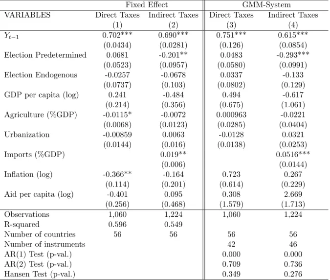
In order to ensure that our results in System-GMM are really reflecting a causality from elections to indirect tax revenues and are not fraught by an endogeneity problem, we follow Brender and Drazen (2005) and Shi and Svensson (2006) by distinguishing the constitutionally determined elections from the endogenous ones. By isolating the strictly exogenous elections, which occurred as constitutionally planned, we make sure that their estimated impact on the different kind of taxes is unbiased. The results are presented in Table 2 and suggest that the previous estimations in GMM-System were correctly dealing with the endogeneity issue because there is a significantly negative effect of the predetermined elections on indirect tax revenues of similar magnitude than previously.
Table 2: Estimation of the election effect on tax structure (direct and indirect taxes as %GDP)
Fixed Effect GMM-System
VARIABLES Direct Taxes Indirect Taxes Direct Taxes Indirect Taxes
(1) (2) (3) (4) Yt−1 0.702*** 0.690*** 0.751*** 0.615*** (0.0434) (0.0281) (0.126) (0.0854) Election Predetermined 0.0681 -0.201** 0.0483 -0.293*** (0.0523) (0.0957) (0.0580) (0.0991) Election Endogenous -0.0257 -0.0678 0.0337 -0.133 (0.0737) (0.103) (0.0802) (0.129)
GDP per capita (log) 0.241 -0.484 0.494 -0.617
(0.214) (0.356) (0.675) (1.061) Agriculture (%GDP) -0.0115* -0.0072 0.000963 -0.0221 (0.0068) (0.0123) (0.0285) (0.0404) Urbanization -0.00859 0.0063 -0.0128 0.0321 (0.0144) (0.016) (0.0138) (0.0253) Imports (%GDP) 0.019** 0.0516*** (0.006) (0.0144) Inflation (log) -0.366** -0.164 0.723 0.267 (0.114) (0.201) (0.614) (0.229)
Aid per capita (log) -0.401 0.095 0.308 2.669
(0.256) (0.468) (1.579) (1.713)
Observations 1,060 1,224 1,060 1,224
R-squared 0.596 0.549
Number of countries 56 56 56 56
Number of instruments 42 46
AR(1) Test (p-val.) 0.000 0.000
AR(2) Test (p-val.) 0.709 0.736
Hansen Test (p-val.) 0.349 0.276
Robust standard errors in brackets. *** p-value<0.01, ** p-value<0.05, * p-value<0.1. Constant and
time fixed effects included in all estimations. GMM-system estimations are two-steps estimations with Windmeijer (2005) finite-sample correction. Urbanization, the agriculture share in GDP, predetermined and
endogenous elections are considered as exogenous; the lagged dependent variable and imports are instrumented with first-order to third-order lags and inflation and GDP are instrumented with second to third-order lagged values. The matrix of instrument has been collapsed.
Again, no significant manipulation of direct taxes is revealed in election years. In developing countries, the incumbent seems therefore more likely to decrease broad-based taxes that could benefit a large number of voters than direct taxes affecting solely firms. Moreover, citizens in developing countries really care about the level of indirect taxes since demonstrations are often happening when some decisions about these taxes seem unfair as in Niger in 2005 where people were in the street during one month to protest against the new dispositions concerning the value added tax.
5
Concluding Remarks
Most studies analysed the presence of political budget cycles in total tax revenues without considering the possibility of an electoral manipulation of specific types of taxes. In this paper we established theoretically, by relying on the political expenditure composition cycle of Drazen and Eslava (2010), the existence of political cycles in the components of taxes. In developing countries, where the median voter’s share of capital is lower than the mean capital endowment of the population, we show that the median voter is more likely to favour low indirect taxes compared to direct taxes. A political cycle will arise in the composition of taxes because voters and politicians have different preferences over tax policy, voters are valuing decreases in indirect taxes whereas politicians prefer decreasing direct taxes in order to favour companies and potentially get contributions. If re-election is valuable enough, a political budget cycle exists with indirect taxes expected to be lower in an election year than in a non-election period. These theoretical prediction were confirmed empirically in a sample of 56 developing countries over the period 1980-2006. Our results reveal significant pre-electoral political budget cycles with non negligible contractions in indirect taxes. No evidence of statistically significant expansions in direct tax revenues were found, they remain unchanged during election periods. By decreasing indirect tax revenues in the election year, governments target the mass of voters rather than firms.
These significant tax cuts in indirect taxes during the election year are an impediment to enhanced tax mobilization, especially in the context of increased democratization in developing countries where more and more elections are held. To limit these detrimental electoral manipula-tions, safeguards should be put in place. Emphasis should be made on fiscal discipline, through regional harmonization for example. WAEMU countries, since 2000, have to comply with the tax policy requirements of the regional union and have therefore less possibilities of electoral manip-ulations. Moreover, strict rules such as deficit and debt limits could also reduce the space for political budget cycles. The prevalence of election-oriented fiscal policies could also be limited with good and strong tax institutions.
References
Adam, C. S., Bevan, D. L., Chambas, G., 2001. Exchange rate regimes and revenue performance in sub-saharan africa. Journal of Development Economics 64 (1), 173–213.
Alesina, A., Rodrik, D., 1994. Distributive politics and economic growth. The Quarterly Journal of Economics 109(2), 465–490.
Alesina, A., Roubini, N., 1992. Political cycles in oecd economies. Review of Economic Studies 59, 663–688.
Alesina, A., Roubini, N., Cohen, G., 1997. Political Cycles and the Macroeconomy. MIT Press, Cambridge, MA.
Andrikopoulos, A., Loizides, I., Prodromidis, K., 2004. Fiscal policy and political business cycles in the eu. European Journal of Political Economy 20, 125–152.
Arellano, M., Bond, S., 1991. Some tests of specification for panel data: Monte carlo evidence and an application to employment equations. Review of Economic Studies 58, 277–297. Arellano, M., Bover, O., 1995. Another look at the instrumental variable estimation of
error-components models. Journal of Econometrics 68, 29–51.
Barro, R., 1973. The control of politicians: an economic model. Public Choice 14, 19–42.
Beck, T., Clarke, G., Groff, A., Keefer, P., W. P., 2001. News tools in comparative political economy: the database of political institutions. World Bank Economic Review 15, 165–176. Block, S. A., 2002. Political business cycles, democratization, and economic reform: the case of
africa. Journal of Development Economics 67, 205–228.
Blundell, R., Bond, S., 1998. Initial conditions and moment restrictions in dynamic panel data models. Journal of Econometrics 87, 115–143.
Brender, A., Drazen, A., 2005. Political budget cycles in new versus established democracies. Journal of Monetary Economics 52, 1271–1295.
Chauvet, L., Collier, P., 2009. Elections and economic policy in developing countries. Economic Policy 24(59), 509–550.
Drazen, A., Eslava, M., 2010. Electoral manipulation via voter-friendly spending: Theory and evidence. Journal of Development Economics 92(1), 39–52.
Fall, E., 2007. Political budget cycle in papua new guinea. IMF WP 07/219.
Gonzalez, M. d. l. A., 2002. Do changes in democracy affect the political budget cycle? evidence from mexico. Review of Development Economics 6(2), 204–224.
Gupta, S., Clements, B., Pivovarsky, A., Tiongson, E. R., 2004. Helping Countries Develop: The Role of Fiscal Policy. Washington: International Monetary Fund, Ch. ”Foreign Aid and Revenue Response: Does the Composition of Aid Matter?”.
Keen, M., Lockwood, B., 2010. The value-added tax: Its causes and consequences. Journal of Development Economics 92(2), 138–151.
Keen, M., Mansour, M., 2009. Revenue mobilization in sub-saharan africa: Challenges from globalization. IMF WP 09/157.
Khattry, B., Rao, J. M., 2002. Fiscal faux pas?: An analysis of the revenue implications of trade liberalization. World Development 30(8), 1431–1444.
Khemani, S., 2004. Political cycles in a developing economy: effect of elections in the indian states. Journal of Development Economics 73, 125–154.
Lindbeck, A., 1976. Stabilization policies in open economics with endogenous politicians. Ameri-can Economic Review Papers and Proceedings, 1–19.
Mikesell, J. L., 1978. Election periods and state tax policy cycles. Public Choice 33 (3), 99–106. Mosley, P., Blessing, C., 2010. The african political business cycle: varieties of experience. paper
presented at Centre for Studies of African Economies conference, Oxford, 21-23 March 2010. Nickell, S., 1981. Biases in dynamic models with fixed effects. Econometrica 49, 1417–1426. Nordhaus, W., 1975. The political business cycle. Review of Economic Studies 42, 169–190. Persson, T., Tabellini, G., 1990. Macroeconomic Policy, Credibility and Politics. Harwood
Aca-demic Publishers, New York NY.
Rogoff, K., 1990. Equilibrium political budget cycles. American Economic Review 80 (1), 21–36. Rogoff, K., Sibert, A., 1988. Elections and macroeconomic policy cycles. Review of Economic
Studies 55(1), 1–16.
Schuknecht, L., 2000. Fiscal policy cycles and public expenditure in developing countries. Public Choice 102, 115–130.
Shi, M., Svensson, J., 2006. Political budget cycles: Do they differ across countries and why? Journal of Public Economics 90, 1367–1389.
Treisman, D., 2007. The Architecture of Government: Rethinking Political Decentralization. Vergne, C., 2009. Democracy, elections and allocation of public expenditures in developing
coun-tries. European Journal of Political Economy 25, 63–77.
Windmeijer, F., 2005. A finite sample correction for the variance of linear efficient two-step gmm estimators. Journal of Econometrics 126, 25–51.
6
Appendices
Appendix 1 - 56 Countries in the sample, type of regime and election years
Argentina (PR) 83, 89, 95, 99, 03 Lesotho (PA) 93, 98, 02
Belize (PA) 84, 89, 93, 98, 03 Madagascar (PR) 82, 89, 93, 96, 01, 06
Bolivia (PR) 80, 85, 89, 93, 97, 02, 05 Malawi (PR) 94, 99, 04
Botswana (PA) 84, 89, 94, 99, 04 Malaysia (PA) 82, 86, 90, 95, 99, 04
Burkina Faso (PR) 91, 98, 05 Mali (PR) 92, 97, 02
Burundi (PR) 84, 93, 05 Mauritania (PR) 92, 97, 03
Cameroon (PR) 80, 84, 88, 92, 97, 04 Mauritius (PA) 82, 87, 91, 95, 00, 05
Cape Verde (PR) 85, 91, 96, 01, 06 Mexico (PR) 82, 88, 94, 00, 06
Central African Rep. (PR) 86, 93, 99, 05 Morocco (PR) 84, 93, 97, 02
Chad (PR) 96, 01, 06 Mozambique (PR) 94, 99, 04
Chile (PR) 89, 93, 00, 06 Niger (PR) 89, 93, 96, 99, 04
Colombia (PR) 82, 86, 90, 94, 98, 02, 06 Nigeria (PR) 83, 93, 99, 03
Congo Rep. (PR) 92, 02 Pakistan (PR) 90, 93, 97
Costa Rica (PR) 82, 86, 90, 94, 98, 02, 06 Peru (PR) 80, 85, 90, 95, 00, 01, 06
Cote d’Ivoire (PR) 80, 85, 90, 95, 00 Philippines (PR) 81, 86, 92, 95, 98, 04
Dominican Rep. (PR) 82, 86, 90, 94, 96, 00, 04 Rwanda (PR) 83, 88, 03
Ecuador (PR) 84, 88, 92, 96, 98, 02, 06 St Vinc.& Grenad. (PA) 84, 89, 94, 98, 01, 05
Egypt Arab Rep. (PA) 84, 87, 90, 95, 00, 05 Senegal (PR) 83, 88, 93, 00
El Salvador (PR) 84, 89, 94, 99, 04 Sierra Leone (PR) 85, 96, 02
Ethiopia (PA) 00, 05 Sri Lanka (PR) 82, 88, 94, 99, 05
Fiji (PA) 82, 87, 92, 99, 01, 06 Sudan (PR) 80, 81, 96, 00
The Gambia (PR) 82, 87, 92, 96, 01, 06 Tanzania (PR) 80, 85, 90, 95, 00, 05
Ghana (PR) 92, 96, 00, 04 Thailand (PA) 83, 87, 92, 95, 96, 01, 05, 06
Guatemala (PR) 82, 85, 90, 95, 99, 03 Togo (PA) 86, 94, 99, 02
Guinea-Bissau (PR) 94, 00, 05 Tunisia (PR) 89, 94, 99, 04
India (PA) 80, 84, 89, 91, 96, 99, 04 Uganda (PR) 96, 01, 06
Iran (PR) 89, 93, 97, 01, 05 Uruguay (PR) 84, 89, 94, 99, 04
Kenya (PR) 83, 87, 92, 97, 02 Zambia (PR) 83, 88, 91, 96, 01, 06
PR: Presidential Regime; PA: Parliamentary Regime in 2000
Appendix 2 - Summary statistics
Variable N Mean Std. Dev. Min. Max.
Indirect Tax (%GDP) 1379 9.101 4.066 .652 31.153 Direct Tax (%GDP) 1201 3.795 1.990 .174 12.0175
Election 1512 .177 .382 0 1
Election Predet 1512 .1237 .329 0 1
Election Endo 1512 .0536 .225 0 1
GDP per capita (log) 1492 7.343 .979 5.278 9.475 Agriculture (%GDP) 1460 25.310 14.205 1.957 72.029
Urbanization 1456 39.702 20.110 4.3 92
Imports (%GDP) 1490 36.608 20.355 2.982 130.923
Inflation (log) 1444 4.122 .413 3.525 9.376