D
D
E
E
P
P
O
O
C
C
E
E
N
N
Working Paper Series No. 2011/07
Growth and convergence in a model with renewable and
non-renewable resources: existence, transitional dynamics, and empirical
evidence
Manh-Hung Nguyen*
Phu Nguyen-Van*
* Toulouse School of Economics, LERNA-INRA
** BETA, CNRS and Université de Strasbourg
The DEPOCEN WORKING PAPER SERIES disseminates research findings and promotes scholar exchanges in all branches of economic studies, with a special emphasis on Vietnam. The views and interpretations expressed in the paper are those of the author(s) and do not necessarily represent the views and policies of the DEPOCEN or its Management Board. The DEPOCEN does not guarantee the accuracy of findings, interpretations, and data associated with the paper, and accepts no responsibility whatsoever for any consequences of their use. The author(s) remains the copyright owner.
Growth and convergence in a model with renewable and
non-renewable resources: existence, transitional dynamics, and
empirical evidence
∗
Manh-Hung Nguyen
a†and Phu Nguyen-Van
b ‡aToulouse School of Economics, LERNA-INRA bBETA, CNRS and Université de Strasbourg
August 21, 2010
Abstract: This paper studies an optimal endogenous growth model using physical capital, labor and two kinds of natural resources in the final goods sector and employing labor to accumulate knowledge. Based on results in calculus of variations, a direct proof of existence of optimal solution is provided. Analytical solutions for the planner case and the balanced growth paths are found for a specific CRRA utility and Cobb-Douglas production function. Transitional dynamics to the steady state from the theo-retical model are used to derive three convergence equations of output intensity growth rate, exhaustible resource growth rate and renewable growth rate, which are tested based on data on production and energy consumption in 27 OECD countries.
Keywords: Optimal growth, existence of equilibrium, transitional dynamics, energy, renewable resource, non-renewable resource.
JEL Classification: C61, D51, E13.
∗We are thankful to Hippolyte d’Albis, Gilles Lafforgue, Cuong Le Van, Francois Salanie for helpful comments and
suggestions. The usual disclaimer applies.
† M.H. Nguyen, Toulouse School of Economics (LERNA-INRA), 21 allée de Brienne, 31000 Toulouse- France. E-mail
address:[email protected]
1
Introduction
An important question that has captivated the attention of environmental economists is whether growth is sustainable in the presence of natural resource scarcity. The issue concerns both academics and public decision-makers, notably in the current context of increasing energy demands and the depletion of fossil fuels expected in the near future. The new growth theory gives the answer that with some technological properties, growth may be sustained in the long-run even if resource stock is finite. This conclusion can be successfully summarized in Smulders (2005): ‘...that a society willing to spend enough on R&D can realize a steady state of technological change sufficient to offset the diminishing returns from capital-resource substitution and sustain long-run growth’, and in Bretschger (2005): ‘...technological change has the potential to compensate for natural resource scarcity, diminishing returns to capital, poor input substitution, and material balance restrictions, but is limited by various restrictions like fading returns to innovative investments and rising research costs.’
However, the literature does not pay enough attention to the existence of the proposed theoretical solution and their empirical justifications. This is particularly due to the difficulty of building a testable version from a complex theoretical framework.
A recent strand of literature concerns the search for empirical evidence for the proposed theoretical models. Pioneer works were done by Brock and Taylor (2004), Alvarez et al. (2005), Bretschger (2006), Miketa and Mulder (2005), and Mulder and De Groot (2007). Brock and Taylor (2004) proposed a Solow growth model with pollution together with empirical justification. They found evidence of an envi-ronmental Kuznets curve (an inverted-U shaped relationship between emissions and income) for OECD countries. They also showed that pollution emissions have a convergence feature, like income convergence in empirical growth studies. Alvarez et al. (2005) provided a Ramsey growth model with pollution which is compatible with the empirical finding about pollution convergence in a panel of European countries. Bretschger (2006) provided an empirical validation of the balanced growth path derived from an endoge-nous growth model with energy. The author also obtained that rising energy prices are not a threat to economic development. Miketa and Mulder (2005) and Mulder and De Groot (2007) found evidence for conditional convergence in energy productivity, i.e. convergence based on country-specific conditions, which seems support the underlying Solow-Swan growth model.
In line with this strand of literature, our paper addresses an endogenous growth model of which the results may be tested with real data. We provide a framework where technological change is endogenized and the production employs labor, physical capital, and both type of renewable and non-renewable resources.1 The roles of renewable and non-renewable resources have been simultaneously analyzed in some recent studies, e.g. Tahvonen and Salo (2001), Gerlagh and van der Zwaan (2003), Tsur and Zemel (2003), André and Cerdá (2006), Grimaud and Rougé (2004, 2005, 2008), Growiec and Schumacher (2008). However, they are mainly related to the substitutability of natural resources (substitution between man-made and natural capitals, substitution between renewable and non-renewable resources) or technological conditions that ensure a sustainable economic growth, and are not explicitly concerned with empirical testing. Our paper investigates a different and more technical issue. We present a rigorous proof of the existence of the optimal solution of a general model, which is often assumed in the many papers in the literature. As always, the arguments for existence of solutions rely on compactness of feasible set and some form of continuity of objective function. We first prove the uniformly boundedness of feasible set (assumptions in d’Albis et al, 2002) that deduces the Lebesgue uniformly integrability. The theorem of Dunford-Pettis ( Dunford-Schwartz (1967)) which characterizes the Lebesgue uniformly integrability and the relatively weak compactness of feasible set is needed in the proof. Then we prove the set of feasible consumption paths is compact. Combined with compactness, upper semi-continuous of objective function is all that is necessary for existence of a maximum. For the proof we also refer the reader to Mazur’s Lemma and Fatou’s Lemma. Next, we propose an analytical model with explicit computation of the transitional dynamics and the balanced growth path. Finally, data on production and energy consumption of OECD countries are used to perform an empirical test based on the transitional equations of this analytical model.
The paper is organized as follows. After the Introduction, in Section 2 we introduce the general optimal endogenous growth model. The existence and uniqueness of a solution is shown in Section 3. A specific model is discussed in Sections 4 where the balanced growth path and analytical optimal growth
1Most of existing studies focus separately renewable and non-renewable resources. However, the literature is very abundant to be cited here. See Kolstad and Krautkraemer (1993), Barbrier (1999), Scholz and Ziemes (1999), Bretschger (2005), Smulders (2005), and Brock and Taylor (2006), among others, for some literature overviews.
rates are found. Section 5 presents the empirical test of the analytical model based on the results of transitional dynamics. Section 6 concludes.
2
The model
The model can be heuristically described as follows. The aggregate output produced from the labor, physical capital and two types of natural resources: non-renewable resources (e.g., fossil fuels) and re-newable resources (solar, thermal, biomass, etc.). The final product is shared between consumption and investment in physical capital. The representative consumer derives her utility from consumption. The production function takes the form
Y =Aθf(K, LY, Q, R)
where A, LY, K, Q and R represent the technological level, labor input, physical capital input, non-renewable resource (or fossil energy), and non-renewable resource (or non-fossil energy), respectively.
We assume the law of motion of technological change is
˙
A= Ψ(A, LA)
where LA is labor employed for research andΨ is a knowledge production function. Normalizing the total flow of labor we have
LY +LA= 1.
The final output can be allocated between consumption and investment (or capital accumulation)
˙
K=Y −C−δK=I−δK,
whereδ∈(0,1)is the depreciate rate of the stock of capital.
It is standard that the dynamics of stock non-renewable resource is following
˙
SQt =−Qt,
whereSQt is the stock of exhaustible resource at timet.It follows from this equation and non-negative restriction onQthat Z
∞
0
Qdt≤SQ0.
The dynamics of stocks of renewable is
˙
SRt =h(SRt)−Rt wherehis a regeneration function.
The representative consumer’s utility function is given by
U = Z ∞
0
u(Ct)e−ρtdt
From now on, as it is not necessary, the time index is not included for simplifying our notation.
3
Existence of optimal solution
In this section, we prove the existence of solution to the social problem (P):
max Z ∞ 0 u(C)e−ρtdt subject to ˙ SR = h(SR)−R, (1) ˙ SQ = −Q, (2) ˙ A = Ψ(A, LA), (3) ˙ K = Aθf(K, L Y, Q, R)−C−δK, (4) LA+LY = 1, (5)
andC≥0, K ≥0, A≥0,0≤LY ≤1,0≤LA≤1, givenA0, LY0, K0, SQ0, SR0.
Note thatθmay be greater than1,the maximal Hamiltonian is not concave in every state variable so the Arrow or Mangasarian sufficiency theorem does not apply in our model. In such an endogenous natural resources dynamic model with non-concave maximal Hamitonian, Kuhn-Tucker first-order conditions together with transversality conditions are necessary and sufficient conditions for an optimal solution is still a conjecture. (see Groth and Schou (2007, footnote 26, p. 93) or Groth and Schou (2002)). As always, the arguments for existence of solutions rely on compactness of feasible set and some form of continuity of objective function. We first prove the uniformly boundedness of feasible set (assumptions in d’Albis et al, 2002) that deduces the Lebesgue uniformly integrability. The theorem of Dunford-Pettis ( Dunford-Schwartz (1967)) which characterizes the Lebesgue uniformly integrability and the relatively weak compactness of feasible set is needed in the proof. Then we prove the set of feasible consumption paths is compact. Combined with compactness, upper semi-continuous of objective function is all that is necessary for existence of a maximum. For the proof we refer the reader to Dunford-Pettis’s Theorem, Mazur’s Lemma and Fatou’s Lemma in the Appendix.
Let us denote by L1(e−ρt) is the set of function f verifying R∞
0 |f(t)|e−ρtdt < ∞. Recall that fi(t) ∈ L1(e−ρt) weakly converges to f(t) ∈ L1(e−ρt) for the topology σ(L1(e−ρt), L∞) (written as
fi * f ) if and only if for everyΨ∈L∞, R∞ 0 fiqe−ρtdt converges to R∞ 0 fΨe−ρtdt as i→ ∞. ( written asR0∞fiΨe−ρtdt−→ R∞ 0 fΨe−ρtdt).
When writingfi−→f∗ we mean that for everyt∈[0,∞),limi→∞fi(t) =f∗(t). We make the following assumptions:
H1. The function u(C) :R+→R is strictly concave, increasing and continuous.
H2. Functions f(K, LY, Q, R) :R4+→R+ is continuously differentiable, increasing on all arguments
and
f(0, .) = 0,
lim
K→+∞fK(K,1, SQ0, SR0) ≤ 0.
H3. FunctionsΨ(A, LA) :R2+→R+is continuously differentiable, increasing in both arguments.Moreover,
there exists a constant b such that
Ψ(A, LA)≤bA.
H4. Functions h(SR) :R+→R+ is continuously differentiable increasing and there exists a constant msuch that h(SR)≤mSR.
H5. There exists κ≥0, κ6=∞, κ≥0, κ6=∞such that−κ≤K/K˙ and−µ≤S˙R/SR,−π≤S˙Q/SQ. H6. ρ >max{b, m, bθ}.
H1-H4 are standards but we do not require the concavity of any function in the technology. Assuming
Ψ(A, LA) ≤ bA has been used in Chichilnisky (1981) and it is weaker than the standard assumption limA→∞ΨA= 0(ΨA= ∂Ψ(∂AA,LA)) and means that after certain levels of technical change the technology is constrained in its knowledge capital increases of productivity by the costs of maintenance, represented by the depreciation parameterb.Similarly for assumption on regeneration functionh.
Assumption H5 is reasonable. It implies that it is not possible that the growth rate of physical capital or stock of renewable resource converges to−∞rapidly and is weaker than those used in the literature whereκis a physical depreciation rate (Chichilnisky (1981), d’Albis et al (2008)). Let us define the net investment : I = ˙K−δK = Aθf(K, L
Y, Q, R)−C. Then H5 implies there exist κ ≥ 0, κ 6=∞ such that I+ (κ−δ)K ≥0.Thus if the standard assumption of non-negative investment holds (that means capital goods cannot be converted back into consumption goods) then H5 holds withκ=δ. Therefore assumption non-negative investment is stronger than A.6 (κcan take any value except for infinity). H4 is similar to A4 in d’Albis et al (2008) which ensures a finite value of objective function and the maximal growth rate of the output is less than discount rate.
Lemma 1 Let us denote byK= (LA, LY, Q, R, SQ, SR, A, K, C)the feasible path fromA0, LY0, K0, SQ0, SR0
which satisfies (1)-(5) and C ≥0, K ≥0, A≥ 0, Q ≥0, R ≥ 0,0 ≤ LY ≤1,0 ≤LA ≤1. Then K is
Proof. By (1) and assumption H4 we haveS˙R≤h(SR)≤mSR and we getS˙R/SR≤m.Thus, there existsS such that
0 ≤ SR≤Semt, ˙
SR ≤ mSemt. (6)
Thus,SRbelongs to the spaceL1(e−ρt)since 0≤ Z ∞ 0 SRe−ρtdt≤S Z ∞ 0 e(m−ρ)tdt <+∞. According to H4,−S˙R≤µSR≤µSemt.It follows from (6) that
¯ ¯ ¯S˙R ¯ ¯ ¯≤max{mS, µS}emt and Z ∞ 0 ¯ ¯ ¯S˙R ¯ ¯ ¯e−ρtdt≤max{mS, µS} Z ∞ 0 e(m−ρ)tdt <+∞. Since0≤R=h(SR)−S˙R≤(m+µ)Semt. Therefore we have
0≤ Z ∞ 0 Re−ρtdt≤(m+µ)S Z ∞ 0 e(m−ρ)tdt <+∞. It follows from (2) that 0 ≤R0tQsds=−
Rt 0S˙Qsds=SQ0−SQ ≤SQ0. Thus ¯ ¯ ¯S˙Q ¯ ¯ ¯ =Q, SQ ≤SQ0
andQ=−S˙Q≤πSQ.We then have Z ∞ 0 SQe−ρtdt ≤ SQ0 Z ∞ 0 e−ρtdt <+∞ Z ∞ 0 Qe−ρtdt = Z ∞ 0 ¯ ¯ ¯S˙Q ¯ ¯ ¯e−ρtdt≤πS Q0 Z ∞ 0 e−ρtdt <+∞.
SincelimK→+∞fK(K,1, SQ0, SR0)≤0, for any ζ∈(0, ρ−bθ)there exist a constantB0such that f(K, LY, Q, R)≤B0+ζK.
It follows that
˙
K≤B0+ζK.
Multiply bye−ζs we gete−ζsK˙ −ζKe−ζs≤B
0e−ζs.Then we get e−ζtK= Z t 0 ∂(e−ζsK) ∂s ds+K0≤ Z t 0 B0e−ζsds+K0=−B0e −ζt ζ + B0+ζK0 ζ .
This implies that there exists constantB1such thatK≤B1eζt. Hence
R∞
0 Ke−ρtdt≤
R∞
0 B1e(ζ−ρ)tdt <
+∞.
Furthermore, since −K˙ ≤κK andK˙ ≤B0+ζK≤B0+ζB1eζt, there exist a constantB2such that
¯ ¯ ¯K˙ ¯ ¯ ¯≤B2eζt. Thus, Z ∞ 0 ¯ ¯ ¯K˙ ¯ ¯ ¯e−ρtdt≤ Z ∞ 0 B2e(ζ−ρ)tdt <+∞.
SinceΨ(A, LA)≤bA,we haveA/A˙ ≤b. There exists a constantD1such thatA≤D1ebt. Moreover,
we have0≤A˙ ≤bA≤D1ebt. Therefore,A, ¯ ¯ ¯A˙ ¯ ¯ ¯belong toL1(e−ρt)because 0 ≤ Z ∞ 0 Ae−ρtdt≤D 1 Z ∞ 0 e(b−ρ)tdt <+∞ 0 ≤ Z ∞ 0 ¯ ¯ ¯A˙ ¯ ¯ ¯e−ρtdt≤D 1 Z ∞ 0 e(b−ρ)tdt <+∞.
As−K˙ ≤κK, we have
C ≤ Aθf(K, LY, Q, R) + (κ−δ)K
≤ D1θebθt(B+ζK) + (κ−δ)B1eζt ≤ D1θebθt(B+ζB1eζt) + (κ−δ)B1eζt
= D1θζB1e(bθ+ζ)t+D1θBebθt+ (κ−δ)B1eζt.
Thus, we can choose a positive constantD2≥D1θB+D1θζB1+ (κ−δ)B1. Then C≤D2e(bθ+ζ)t< D2eρt, which implies 0≤ Z ∞ 0 Ce−ρtdt <+∞.
We have proven that Kis uniformly bounded onL1(e−ρt). Moreover, lima→∞
R∞
a Ke−ρtdt ≤lima→∞ R∞
a B1e(ζ−ρ)tdt = 0. This property is true for other vari-ables inK. ThereforeKsatisfies Dunford-Pettis theorem and it is relatively compact in the weak topology
σ(L1(e−ρt), L∞).
SinceKis relatively compact in the weak topologyσ(L1(e−ρt), L∞),a sequenceX
iinKhas convergent subsequences (denote byXi for simplicity of notation) which weakly converge to limit points inL1(e−ρt). The following Lemma shows that any weakly convergent sequence of control variables in K has a sequence of convex combinations of its members that converges pointwise to the same limit while the limit of weak convergence coincide with limit of pointwise convergence for state variables.
Lemma 2 i)Let(K, A, SR, SQ)i inK and suppose that(K, A, SR, SQ)i*(K∗, A∗, SR∗, SQ∗).
Then (K, A, SR, SQ)i→(K∗, A∗, SR∗, SQ∗)as i→ ∞and( ˙K,A,˙ S˙R,S˙Q)i *( ˙K∗,A˙∗,S˙R∗,S˙Q∗) for the
the topologyσ(L1(e−ρt), L∞).
ii) In addition, suppose thatZi= (R, Q,K,˙ A,˙ S˙R,S˙Q)iinKandZi*Z∗= (R∗, Q∗,K˙∗,A˙∗,S˙R∗,S˙Q∗)
in L1(e−ρt) then there exists a sequence of sets of real numbers {ω
i(n) | i = n, ...,N(n)} such that ωi(n)≥0 and
PN(n)
i=n ωi(n)= 1 such that the sequence (vn)n∈N defined by the convex combinationvn = PN(n)
i=n ωi(n)Zi converges pointwise to Z∗ as n→ ∞, i.e., for everyt∈[0,∞),limn→∞vn(t) =Z∗(t). It
is clearly that, since (LA, LY,)i(n)∈[0,1],(LA, LY,)i(n)→(L∗A, L∗Y)asn→ ∞. Proof. For anyXi∈ K.We first claim that, for t∈[0,∞),
Rt
0Xidt→
Rt
0X∗dt.Note thatXi * X∗
for the topologyσ(L1(e−ρt), L∞)if and only if for everyY ∈L∞,R∞
0 XiY e−ρtdt→
R∞
0 X∗Y e−ρtdt.
Pick anytin [0,∞)and let
Y(s) =
½ 1
e−ρt ifs∈[0, t]
0ifs > t.
Therefore Y(s) ∈ L∞ and we get Rt
0Xi(s)ds = R∞ 0 Xi(s)Y(s)e−θsds → R∞ 0 X∗(s)Y(s)e−θsds = Rt 0X∗(s)ds.
Given thatKi * K∗ andK˙i* y weakly inL1(e−ρt),by the claim above, for all t∈[0,∞)we have Rt
0Kids→
Rt
0yds. This implies, for a fixt, Ki→
Rt
0yds+K0.Thus
Rt
0yds+k0=K∗. ThereforeK˙∗=y
orK˙i*K˙∗.The same reasoning applies for(A, SR, SQ)i inK. ii) A direct application of Mazur’s Lemma.
We are now able to prove the existence of solution to the to the social planner’s problem.
Theorem 1 Under Assumptions H.1-H.7, there exists a solution to the social planner’s problem.
Proof. Since uis concave, for any c >¯ 0, u(C)−u(¯c) ≤u0(¯c)(C−¯c). Thus, ifC ∈L1(e−ρt)then R∞
0 u(C)e−ρtdtis well defined because
Z ∞ 0 u(C)e−ρtdt≤ Z ∞ 0 [u(¯c)−u0(¯c)¯c]e−ρtdt+u0(¯c) Z ∞ 0 Ce−ρtdt <+∞.
Let us define W = supC∈K
R∞
0 u(C)e−ρtdt. Assume thatW > −∞(otherwise the proof is trivial).
LetCi ∈ Kbe the maximizing sequence of R∞
0 u(C)e−ρtdtso limi→∞
R∞
0 u(Ci)e−ρtdt=W.
Since K is relatively weak compact, suppose that Ci * C∗ for some C∗ in L1(e−ρt). By Mazur’s Lemma, there is a sequence of convex combination
xn= NX(n) i=n ωi(n)Ci(n)→C∗, ωi(n)≥0, NX(n) i=n ωi(n)= 1.
Because uis concave, we have
lim sup n→∞u(xn) = lim supn→∞u( NX(n) i=n ωi(n)Ci(n)) ≤ lim sup n→∞[u(C ∗) +u0(C∗)( NX(n) i=n ωi(n)Ci(n)−C∗)] =u(C∗).
Since this holds for almost t,integrate w.r.t e−ρtdt to get Z ∞ 0 lim sup n→∞u(xn)e −ρtdt≤ Z ∞ 0 u(C∗)e−ρtdt <+∞. Using a reverse Fatou’s lemma (see Appendix) we yield
lim sup n→∞ Z ∞ 0 u(xn)e−ρtdt≤ Z ∞ 0 lim sup n→∞u(xn)e −ρtdt≤ Z ∞ 0 u(C∗)e−ρtdt. (7) Moreover, by Jensen’s inequality we get
lim sup n→∞ Z ∞ 0 u(xn)e−ρtdt≥lim sup n→∞ NX(n) i=n ωi(n) Z ∞ 0 u(Ci(n))e−ρtdt. (8)
But since R0∞u(Ci(n))e−ρtdt→W, (7) and (8) imply
R∞
0 u(C∗)e−ρtdt≥W.
So it remains to show thatC∗ is feasible.
The task is now to show that there exists some (K∗, L∗
A, L∗Y, A∗, R∗, Q∗, S∗R, SQ∗) in K such that (C∗, K∗, L∗
A, L∗Y, A∗, R∗, Q∗, SR∗, SQ∗)satisfies (1)-(4).
Consider a feasible sequence(K, LA, LY, A, R, Q, SR, SQ)i(n)inKassociated withCi(n).According to
Lemma2 and Jensen’s inequality we have
C∗ = lim n→∞xn= limn→∞ NX(n) i=n ωi(n)Ci(n) ≤ lim n→∞ NX(n) i=n ωi(n)[Aθif(Ki, LYi, Qi, Ri)−δKi−K˙i] = lim n→∞ NX(n) i=n
ωi(n)[ limn→∞Aθif( limn→∞Ki(n),nlim→∞LYi, Qi, Ri)−δnlim→∞Ki(n)]−nlim→∞
NX(n) i=n ωi(n)K˙i ≤ A∗θf(K∗, L∗Y,nlim→∞ NX(n) i=n ωi(n)Qi, lim n→∞ NX(n) i=n ωi(n)Ri)−δK∗− lim n→∞ NX(n) i=n ωi(n)K˙i = A∗θf(K∗, L∗Y, Q∗, R∗)−δK∗−K˙∗. Therefore, C∗≤A∗θf(K∗, L∗ Y, Q∗, R∗)−δK∗−K˙∗.
Applying a similar argument and using Jensen’s inequality we get ˙ A∗ = lim n→∞ NX(n) i=n ωi(n)A˙i(n)= NX(n) i=n ωi(n)Ψ( limn→∞Ai, lim n→∞LAi) = Ψ(A ∗, L∗ A), ˙ S∗ R = nlim→∞ NX(n) i=n ωi(n)S˙Ri = limn→∞ NX(n) i=n ωi(n)(h(SRi)−R) =h(S ∗ R)−R∗, ˙ S∗ Q = nlim→∞ NX(n) i=n ωi(n)S˙Qi =−nlim→∞ NX(n) i=n ωi(n)Qi=−Q∗ Therefore,(C∗, K∗, L∗ A, L∗Y, A∗, R∗, Q∗, SR∗, SQ∗)satisfies (1)-(4). The proof is done.
Our proof is adapted from works of Chichilnisky (1981) and d’Albis et al (2008) to the endogenous technical change model with less stringent assumptions. The technology is not convex in our model ( d’Albis et al (2002) assumed the technology is convex w.r.t consumption). We prove that the control variable (as consumption C ) and derivative of state variables weakly converge in the weak topology
σ(L1(e−ρt), L∞), while the state variables pointwise converge. And for pointwise converge sequence, the
continuity is all that is necessary to prove the feasibility. Therefore, concavity is not needed for the state variables. Related results on the existence of solution can be found in Chichilnisky (1981) who used the theory of Sobolev weighted space and imposed a Caratheodory condition on utility function.
Once the existence of solution is proven, the solution is unique if utility function is strictly concave and technology is convex. This enable us to derive sufficient conditions for opimality. In other words, the Kuhn-Tucker first-order conditions together with transversality conditions are necessary and sufficient conditions for an optimal solution.
Define σC=−CUUCCc be the elasticity of marginal utility and F =Aθf(K, LY, Q, R).
We have proven that (P) has a solution. Then the necessary conditions are characterized by the Kuhn-Tucker conditions. By setting the current-value Hamiltonian,
H(C, K, Q, R, LY, A) =u(C) +λ[h(SR)−R]−µQ+ν(F−C−δK) +ωΨ(A, LA) whereλ, µ, ν, ω are four costate variables, the first order conditions (∂H
∂C = 0, ∂H∂Q = 0,∂H∂R = 0,∂L∂HY = 0) yield ν = UC, µ = vFQ, λ = vFR, ω = vFLY ΨLA .
From Euler equations ∂H
∂K =ρν−ν,˙ ∂S∂HR =ρλ− ˙ λ, ∂H ∂SQ =ρµ−µ,˙ and ∂H ∂A =ρω−ω˙ we get ˙ ν = (ρ−FK+δ)v ˙ µ = ρµ ˙ λ = (ρ−hSR)λ ˙ ω = (ρ−ΨA)ω−vFA. The transversality conditions are
lim t→+∞λSRe −ρt= lim t→+∞µSQe −ρt= lim t→+∞νKe −ρt= lim t→+∞ωAe −ρt= 0.
Moreover, it is easy to see that, at the optimum, the Ramsey conditions and Hotelling rules are satisfied. ρ+σC ˙ C∗ C∗ =FK−δ= ˙ FQ FQ = F˙R FR +hSR = ˙ FLY FLY −g˙LA gLA +gA+ FAgLA FLY .
4
Characterization of balanced optimal growth paths
Before analyzing the full dynamic system, we look at the characterization of a balanced optimal growth path. The model in Section 2 corresponds to a system with four state variables. As Kolstad and Krautkraemer (1993) remarked, ‘...it is difficult or impossible to characterize the qualitative features of a dynamic model evolving three state variables without restrictive assumptions about the functional forms of important relationships...’, we specify a set of restrictions imposed on preferences and production technology in order to have analytical results that may be tested with real data. We make the following assumptions: H7. u(C) = ½ C1−ε−1 1−ε , ifε6= 1, lnC ifε= 1. , H8. f(LY, K, Q, R) =LγYKξQαRβ whereγ, ξ, α, β≥0, γ+ξ+α+β= 1. H9. Ψ(A, LA) =bAφLAwhereb >0,0< φ≤1 H10. h(SR) =mSR, m >0.
This specification satisfies H1-H6. H9 is widely used in the literature (see, e.g., Aghion and Howitt, 1998, Jones, 2006). Assumption H10 allows for constant infinite growth for renewable which is not realistic for ecological restriction. However, it may be reasonable for a type of of non-fossil energy such as solar energy, wind energy or nuclear energy in which the stock of alternative energy can be considered as infinity.
Let gχ = ˙χ/χ denote the growth rate of any variable χ. We shall summarize the macroeconomic equilibrium in terms of five variables: x=F/K, y=C/K, z =Q/SQ, u=R/SR, q=LYAφ−1, r=Aφ−1 from which other equilibrium ratesgF, gK, gC, gLY, gLA, gA, gQ, gSQ, gR, andgSRcan be derived as in the following proposition.
Proposition 1 The optimal growth rates take the following values
gA = b(r−q), gK = x−y−δ, gC = ξx−δ−ρ ε , gSQ = −z, gSR = m−u, gQ = −y+bθr ξ + mβ+ (1−ξ)δ ξ , gR = −y+bθr ξ + m(β+ξ) + (1−ξ)δ ξ , gLY = −y+ bθr ξ + bθ γq+ mβ+ (1−ξ)δ ξ , gF = ξx−y+bθr ξ + mβ+δ(α+β+γ) ξ −δ, gLA = q q−rgLY.
Proof. See Appendix
A steady state satisfies that all rates of growth are constant. Letχ∗ andg∗
χ denote respectively the value and the growth rate of any variableχat the steady state.
Proposition 2 At the steady state, the growth rates take the following values g∗Q = g∗SQ =−y ∗+bθr∗ ξ + mβ+ (1−ξ)δ ξ , g∗ R = g∗SR=−y ∗+bθr∗ ξ + m(β+ξ) + (1−ξ)δ ξ , gF∗ = g∗K=gC∗ = ξx∗−δ−ρ ε , g∗ LY = g ∗ LA= 0, g∗ A = b(r∗−q∗), where if φ= 1then x∗ = bθ+mβ+δ(1−ξ) ξ(1−ξ) , y∗ = (ε−ξ)(bθ+mβ+δ(1−ξ)) +ξ(1−ε)δ+ρ] εξ(1−ξ) , q∗ = [y∗−mβ+ (1−ξ)δ+bθ ξ ] γ θb, r∗ = 1,
and if φ <1 thenx∗, y∗, q∗, r∗ are given by
ξx∗−δ−ρ ε = x ∗−y∗−δ, (ξ−1)x∗−y∗+δ+bθq∗+mβ+δ(1−2ξ) ξ = 0, (9) −y∗+mβ+ (1−ξ)δ+bθq ∗ ξ + bθ γq ∗ = 0, (10) r∗ = q∗.
Proof. See Appendix
Remark 2 We have z∗ =−g∗
SQ, u
∗ =m−g∗
SR. It follows from transversality conditions at the steady state and the Euler equation thatlimt→+∞µSQ∗e−ρt= 0whereµ=µ(0)e−ρtandSQ∗(t) =SQ∗(0)eg
∗
Qt. We then obtain limt→+∞µ(0)SQ∗(0)eg
∗
Qt= 0. This implies g∗
Q <0. Similarly, since limt→+∞λSRe−ρt = 0
whereλ=λ(0)e(ρ−m)t, we getlim
t→+∞λ(0)SR∗(0)e(g ∗ R−m)t= 0or g∗ R−m <0.
5
Econometric estimation
5.1
Estimated equations
We first study the dynamic behavior of the nonlinear system which is characterized by the behavior of the linearized system around the steady state.We shall summarize the macroeconomic equilibrium in terms of four stationary variables, x= F/K, y =C/K, z =Q/SQ, u = R/SR, q = Aφ−1LY, r =Aφ−1, from which other equilibrium rates can be derived as in Proposition 1. Let us denoteh= (x, y, z, u, q, r). From the theory of linear approximation we know that in the neighborhood of the steady state, the dynamic behavior of the nonlinear system is characterized by the behavior of the linearized system around the steady state ˙h=J(h−h∗)whereh∗= (x∗, y∗, z∗, u∗, q∗, r∗)andJis the Jacobian matrix evaluated at
the steady state, i.e.
J= ∂x/∂x ∂˙ x/∂y ∂˙ x/∂z ∂˙ x/∂u ∂˙ x/∂q ∂˙ x/∂r˙
∂y/∂x ∂˙ y/∂y˙ ∂y/∂z˙ ∂y/∂u ∂˙ y/∂q˙ ∂y/∂r˙
∂z/∂x˙ ∂z/∂y˙ ∂z/∂z˙ ∂z/∂u˙ ∂z/∂q˙ ∂z/∂r˙
∂u/∂x ∂˙ u/∂y ∂˙ u/∂z ∂˙ u/∂u ∂˙ u/∂q ∂˙ u/∂r˙
∂q/∂x˙ ∂q/∂y˙ ∂q/∂z˙ ∂q/∂u˙ ∂q/∂q˙ ∂q/∂r˙ ∂r/∂x˙ ∂r/∂y˙ ∂r/∂z˙ ∂r/∂u˙ ∂r/∂q˙ ∂r/∂r˙ .
Proposition 3 If φ= 1 then the Jacobian matrix has only one negative eigenvalue. If φ <1 then the Jacobian matrix has at most two negative eigenvalues.
Proof. see Appendix.
Remark 3 Let vi, i = 1, ...,6, denote the eigenvectors corresponding to six eigenvalues λi. We may
write the general solution of ˙h=J(h−h∗), where h∗= (x∗, y∗, z∗, u∗, q∗, r∗), as follows:
h(t)−h∗=
6
X i=1
aivieλit
where parameters ai are determined by the initial conditions h(0)−h∗ = P6
i=1aivi. The optimal path
in the neighborhood of the steady state is located in the stable subspace which corresponds to the negative eigenvalues. Thus, ifφ= 1, we can writeh(t)−h∗=c
1v1eλ1t whereλ1<0.
We are now in a position to discuss about the empirical implication of the theoretical model. We focus our analysis on the growth rates gF/K, gQ, and gR at the transition path. We only consider the caseφ= 1, where all of these growth rates only depend onx≡F/K andy≡C/K.2 From the previous analysis forφ= 1, as the components ofhare independent of each other, we can write the approximation expressions forxandy as follows
xt−x∗ = c1v1xeλ1t, (11)
yt−y∗ = c1v1yeλ1t, (12)
wherev1x andv1y, two components ofv1. By using the initial conditions, we get c1v1x = x0−x∗
c1v1y = y0−y∗
Therefore, we obtain the following solution
xt = (1−eλ1t)x∗+eλ1tx0, (13) yt = (1−eλ1t)y∗+eλ1ty0. (14)
Recall that we have
gx = (ξ−1)x+bθ+mβ+δ(1−ξ) ξ , gQ = −y+bθ ξ + mβ+ (1−ξ)δ ξ , gR = −y+bθ ξ + m(β+ξ) + (1−ξ)δ ξ .
We substitute (13) and (14) in these expressions and use definitions x0 = F0/K0, y0 = C0/K0,
and gx =gF/K = T1ln(FT/F0)−T1ln(KT/K0), gQ = T1 ln(QT/Q0) andgR = T1ln(RT/R0), which are
respectively the average growth rates ofF/K,Q, andR, between 0 andT. This results in the transitional dynamics ofgχ, χ=F/K, Q, Rtowards the steady-state of the economy.3
First,gF/K is given by4 gF/K = (ξ−1)xT +bθ+mβ+δ(1−ξ) ξ = bθ+mβ+δ(1−ξ) ξ + (ξ−1)(1−e λ1T)x∗+ (ξ−1)eλ1Tx 0 = α0+α1F0/K0+εF/K, (15)
2It should be noticed that whenφ <1, the model is not identified and then estimation becomes impossible unless some restrictions are imposed.
3The reason of usingg
F/Kinstead ofgF is that the approximation of the latter contains in the right-hand side bothF/K andC/Kwhich are highly correlated. Hence, regression ofgF onF/KandC/Kwill face a problem of multicolinearity.
with α0 = bθ+mβ+δ(1−ξ) ξ + (ξ−1)(1−e λ1T)x∗, α1 = (ξ−1)eλ1T. ConcerninggQ, we have gQ = −(1−eλ1T)y∗−eλ1Ty0+bθ ξ + mβ+ (1−ξ)δ ξ = β0+β1C0/K0+εQ, (16) where β0 = −(1−eλ1T)y∗+bθ ξ + mβ+ (1−ξ)δ ξ , β1 = −eλ1T. Similarly, gR is given by gR = −y+bθ ξ + m(β+ξ) + (1−ξ)δ ξ = −(1−eλ1T)y∗−eλ1Ty 0+bθ ξ + m(β+ξ) + (1−ξ)δ ξ = γ0+γ1C0/K0+εR, (17) where γ0 = bθ ξ + m(β+ξ) + (1−ξ)δ ξ −(1−e λ1T)y∗, γ1 = −eλ1T.
Equations (15), (16), and (17) represent three cross-sectional regressions where εF/K andεQ and εR are the corresponding error terms.5 These equations may be estimated by using Ordinary Least Squares as in Mankiw et al. (1992). However, as underlined by Islam (1995) and subsequent studies on income convergence, we will lose information contained by the data as we only need observations of the initial and final dates, i.e. dates 0 andT, and the sample size is then reduced to to the number of countries.
An alternative approach is to transform the model in a panel structure. In particular, we can rewrite equations (15), (16), and (17) as follows:
g(F/K)it = α0+α1Fi,t−1/Ki,t−1+ε(F/K)it, (18)
gQit = β0+β1Ci,t−1/Ki,t−1+εQit, (19)
gRit = γ0+γ1Ci,t−1/Ki,t−1+εRit, (20) wherei= 1, ..., N, and t= 1, ..., T. As in most studies on income convergence (see Durlauf et al., 2005, for a survey), we use data corresponding to the five year interval period, i.e. data from 1977, 1982, 1987, 1992, and 1997. Hence the length betweentandt−1is equal to 5 andgχit =
1
5ln(χt/χt−1). The purpose
is to reduce the business cycle effect.
The sample size is 108 observations (N = 27, T = 4). In our panel data framework, the error terms
εχit,χ=F/K, Q, R, include country and time effects, i.e. εχit =µi+λt+uχit where µi andλtdenote country heterogeneity and time heterogeneity respectively, anduχit is the idiosyncratic error. Moreover, the model predicts that coefficientsα1,β1, andγ1 are negative.
Estimations of these equations can be obtained with standard panel methods (within estimation for fixed effects, Generalized Least Squares for random effects) which assume the strict exogeneity of regressors, i.e.
E[(Fs/Ks)ε(F/K)t] =E[(Cs/Ks)εQt] =E[(Cs/Ks)εRt] = 0,∀s, t.
5These error terms may correspond to omitted variables or unobserved factors that can affect the growth ratesgF/K,
However, this assumption may be faulty as regressors can be correlated with some unobserved factors or with future values of the dependent variable. This is probably the case when we study macroeconomic data. For example, we may think that current consumption and capital stock may have some impacts not only on current income and energy consumption but also on their future values. This situation arises when regressors arepredetermined, i.e.
E[(Fs/Ks)ε(F/K)t] =E[(Cs/Ks)εQt] =E[(Cs/Ks)εRt] = 0,∀s < t−1.
In this case, the model can be estimated by using Generalized Methods of Moments (see, e.g., Arellano and Bond, 1991, Baltagi, 2005, and Lee, 2002). This is also the approach adopted in our estimation strategy.
5.2
Data
The data covers twenty-seven OECD countries for the period 1977-1997.6 Data on non-renewable energy consumptionQand renewable energy consumptionRare collected from the International Energy Agency (IEA). Non-renewable energy consumption,Q, is measured as the sum of consumption of gas, and liquid fuels (in metric tons oil equivalent, toe). We assume that renewable energy consumption,R, corresponds to the sum of nuclear energy, hydroelectricity, geothermal energy, renewable fuels and waste, solar energy, wind energy, and energy from tide, wave, and ocean (also in toe).
Data on productionF, consumptionC, physical capital stock K, and population are collected from the Penn World Table 6.1 (Heston et al., 2002). We note that all figures, except population, are expressed in PPP and 1996 prices for an international comparison purpose. We use the population series and the series on real GDP per capita in 1996 prices (series RGDPL) to produce the volume of real GDP in 1996 prices. We compute the product between real GDP and investment share of real GDP on the one hand, and the product between real GDP and consumption share of real GDP on the other hand, which correspond respectively to investment and consumption in real terms. Calculation of physical capital stock is based on the investment series (i.e. investment share of real GDP) following the perpetual inventory method.7 Data are used in per capita terms to neutralize the possible scale effect due to the difference in population size observed between countries.
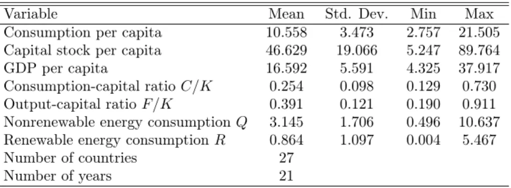
Table 1 here
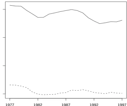
Descriptive statistics of the data are summarized in Table 1. Evolutions of the averages of ratios
F/K and C/K are displayed in Figure ??. These ratios have similar patterns, with two dips around 1982 and 1993, except that F/K has stronger variation thanC/K (standard deviation of F/K, 0.121, is higher than that of C/K, 0.098). Series on consumptions of nonrenewable and renewable resources are presented in Figure ??. The average of consumption of renewable energies R, is much lower than that of nonrenewable energiesQ, which increased over the whole period of the study whereas the latter considerably decreased in the late 70s until the dip in 1983 and then increased thereafter.
Figures??-??here
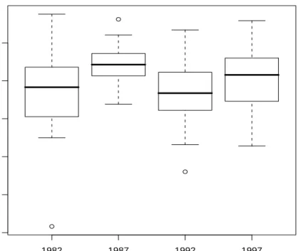
For the estimations, we take data corresponding to the five year interval period (data from years 1977, 1982, 1987, 1992, and 1997) in order to eliminate business cycle effects as in most of empirical studies on economic convergence. Distributions of average annual growth rates (computed from these time intervals) of the output to capital ratioF/K,gF/K, renewable energy consumption per capita,gR, and nonrenewable energy consumption per capita,gQ, are reported in Figures??,??, and??, respectively. The distribution of these growth rates sensitivity changes over time. We also observe a particularity that the dispersion ofgQ andgRdiminishes throughout the period of study.
6The data include Australia, Austria, Belgium, Canada, Denmark, Finland, France, Germany, Greece, Hungary, Iceland, Ireland, Italy, Japan, Korea, Luxembourg, Mexico, the Netherlands, New Zealand, Norway, Portugal, Spain, Sweden, Switzerland, Turkey, United Kingdom, and the United States.
7The perpetual inventory equation isK
t=It+ (1−δ)Kt−1 whereIt is the investment flow. The initial capital stock is given by K0 =I0/(gI+δ) where gI is the average geometric growth rate of investment from the initial date. The depreciation rate,δ, is often set to 4 to 6%. In our paper, changingδ from 4% to 6% does not modify the qualitative conclusion.
5.3
Estimation results
Estimation results by GMM are reported in Table 2. As GMM use the first-difference transformation, the intercept and country effects (which are not separately identified) are deleted from the regressions and therefore not estimated. Furthermore, the assumption of predetermined regressors,
E[(Fs/Ks)ε(F/K)t] =E[(Cs/Ks)εQt] =E[(Cs/Ks)εRt] = 0,∀s < t−1,
allows us to use all values of Fs/Ks and Cs/Ks, s= 1, ..., t−2, as possible instruments forFt/Kt and
Ct/Kt, respectively. As a consequence, there are finally 81 observations used in the estimations.
Table 2 here
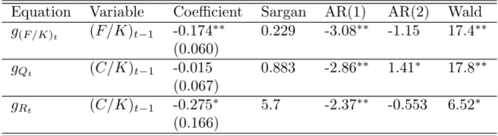
Empirical results based on OECD data confirm the prediction of the theoretical model. Indeed, estimation results show that coefficients α1, β1, and γ1 are negative as expected. Coefficients α1 and γ1 are statistically significant at the 5% and the 10% levels respectively, while β1 is insignificant. The
Wald test confirms the existence of time effects in all regressions. The Sargan specification test for over-identifying restrictions (relative to the use of instrumental variables) is always satisfied in either regressions as these over-identifying restrictions are not rejected.
It should be noted that the GMM estimator is consistent with an AR(1) process for the regression residuals but not consistent with an AR(2). We use the Arellano-Bond (1991) tests to examine this issue. Test results reject the absence of autocorrelation of order 1 but do not reject that of order 2 for regressions withgF/K andgR, suggesting that estimations are consistent in these cases. Concerning gQ, the specification does not seem robust as Arellano-Bond test does not confirm (but only at the 10% level) the absence of an AR(2) process in the residuals.
6
Conclusion
The paper is an attempt to explore theoretically and empirically the interaction between growth, techno-logical level, and consumptions of renewable and non-renewable resources. The necessary and sufficient conditions are provided in a general endogenous growth model. We also characterize the BGP together with the transitional dynamics for an analytical model which are shown helpful for empirical analysis by using panel data on OECD countries. Our estimation strategy is appealing since it accounts for country and time heterogeneities and it allows for a more flexible assumption about regressors than the usual assumption of strictly exogenous regressors in the standard framework.
As underlined previously, it would be of particular interest, in a further work, to study the identifi-cation issue of the empirical specifiidentifi-cation that can be derived from the theoretical model whenφ <1 or from a more general model. Moreover, it would be promising to consider externalities from resource use in utility or production in order to improve the realism of the modeling. Competitive equilibrium and public policy would also require a particular attention.
Appendix
The following theorem and lemmas are used in the proof of existence of an optimal solution.
Let F be a family of scalar measurable functions on a finite measure space (Ω,Σ, µ), F is called uniformly integrable if{RE|f(t)|dµ, f ∈F}converges uniformly to zerowhen µ(E)→0.
Dunford-Pettis Theorem: Denote L1(µ)the set of functions f such that R∞
0 |f|dµ <∞ and K
be a subset of L1(µ).Then K is relatively weak compact if and only if K is uniformly integrable.
The following is the reverse Fatou’Lemma when applying Fatou’s lemma to the non-negative sequence given byg−fn.
Fatou’s Lemma: Let fn be a sequence of extended real-valued measurable functions defined on a
measure space (Ω,Σ, µ). If there exists an integrable function g on Ω such that fn ≤g for all n, then lim supn→∞
R
Ωfndµ≤
R
Ωlim supn→∞fndµ.
Mazur’s lemma shows that any weakly convergent sequence in a normed linear space has a sequence of convex combinations of its members that converges strongly to the same limit. Because strong convergence is stronger than pointwise convergence, it is used in our proof for state variables converge pointwise to the limit obtained from weak convergence.
Mazur’s Lemma: Let (X,|| ||) be a normed linear space and let (un)n∈N be a sequence in X that
converges weakly to someu∗in X. Then there exists a function N : N→N and a sequence of sets of real
numbers{ωi(n)|i=n, ...,N(n)}such thatωi(n)≥0and
PN(n)
i=n ωi(n)= 1such that the sequence(vn)n∈N
defined by the convex combination vn= PN(n)
i=n ωi(n)ui converges strongly in X to u∗,i.e.,||vn−u∗|| →0 asn→ ∞.
Under assumptions H11-H13, the program of the social planner can be written as follows
max Z ∞ 0 u(C)e−ρtdt subject to F = AθLγ YKξQαRβ, ˙ SQ = −Q, ˙ SR = mSR−R, ˙ K = F−C−δK, ˙ A = bAφL A, 1 = LA+LY, LY0, K0, SQ0, SR0 given. Proof of Proposition 1
Proof. The current-value Hamiltonian is
H(C, K, Q, R, LY, A) = u(C) +λ(mSR−R)−µQ
+ν(F−C−δK) +ωbAφ(1−LY) whereλ, µ, ν, ω are four costate variables.
The first order conditions ∂H
∂C = 0, ∂H∂Q = 0,∂H∂R = 0,∂L∂HY = 0yield ν = UC, (21) µ = vFQ, (22) λ = vFR, (23) ω = vFLY bAφ . (24)
From Euler equations ∂H∂K =ρν−ν,˙ ∂S∂H R =ρλ− ˙ λ,∂S∂H Q =ρµ−µ,˙ and ∂H ∂A =ρω−ω˙ we get ˙ ν v = ρ−FK−δ (25) ˙ µ µ = ρ (26) ˙ λ λ = ρ−m (27) ˙ ω = (ρ−bφAφ−1(1−L Y))ω−vFA. By (21) andA/A˙ =bAφ−1(1−L Y)we get ˙ ω= (ρ−φgA)ω−UCFA. (28)
The transversality conditions are
lim t→+∞λSRe −ρt= lim t→+∞µSQe −ρt= lim t→+∞νKe −ρt= lim t→+∞ωAe −ρt= 0. From the identities S˙R=mSR−R,S˙Q=−QandK˙ =F−C−δK, we obtain
gSQ = −z, gSR = m−u, gK = x−y−δ, gA = b(r−q). SinceF =AθLγ YKξQαRβ,we have FK=ξF/K =ξx, ˙ FQ FQ = θgA+γgLY +ξgK+ (α−1)gQ+βgR, (29) ˙ FR FR = θgA+γgLY +ξgK+αgQ+ (β−1)gR, (30) ˙ FLY FLY = θgA+ (γ−1)gLY +ξgK+αgQ+βgR (31) Equation (21) together with (25) yield
ρ−U˙C
UC
=FK−δ=ξx−δ. (32)
It is easy to check that
˙ UC UC =−ε ˙ C C =−εgC. (33) Thus, gC= ξx−δ−ρ ε .
By logarithmic differentiation (22) and together with (26) we have
˙ FQ FQ =ρ− ˙ UC UC =ξx−δ. From (23) and (27) we get
˙ FR FR =ρ− ˙ UC UC −m=ξx−δ−m.
From (24) and (28) we get ˙ UC UC + ˙ FLY FLY −φgA = ρ−φgA− UCFA ω = ρ−φgA− UCFA UCFLY Aφ = ρ−φg A− θF/A γF/LYA φ= ρ−φgA−θ γLYA φ−1 = ρ−φg A−bθ γq. Thus, ˙ FLY FLY =ρ−U˙C UC −bθ γq=ξx−δ− bθ γq.
Now, it follows from (29)-(31) that we have a system of equations with three variables gQ, gR, and
gLY: γgLY + (α−1)gQ+βgR = ξy−bθ(r−q) + (ξ−1)δ=T1, (34) γgLY +αgQ+ (β−1)gR = ξy−m−bθ(r−q) + (ξ−1)δ, (35) (γ−1)gLY +αgQ+βgR = ξy− bθ γq−bθ(r−q) + (ξ−1)δ. (36) From (34)-(35) we have−gQ+gR=m.
From (34)-(36) we get γgLY =bθq+γgQ. Replacing this equation into (34), we have
(γ+α−1)gQ+βgR=T1−bθq
We then have two equations to findgQ andgR:
gQ = mβ+bθq−T1 ξ = bθr−ξy+mβ+ (1−ξ)δ ξ , gR = gQ+m= bθr−ξy+m(β+ξ) + (1−ξ)δ ξ , and gLY = bθ γq+gQ= bθr−ξy+mβ+ (1−ξ)δ ξ + bθ γq. By log-differentiatingF =AθLγ YKξQαRβ we get gF = θgA+γgLY +ξgK+αgQ+βgR= = γgLY + (α−1)gQ+βgR+θgA+ξgK+gQ = T1+θgA+ξgK+gQ = ξy+ (ξ−1)δ+ξ(x−y−δ) +bθr−ξy+mβ+ (1−ξ)δ ξ = ξx−y+bθr ξ + mβ+δ(1−2ξ) ξ = ξx−y+bθr ξ + mβ+δ(α+β+γ) ξ −δ. Finally, sinceLY = qr, gLA= ˙ LA LA =− L˙Y 1−LY = LY LY −1 gLY = q q−rgLY. Proof of Proposition 2
Proof. At the steady state,g∗
A=b(r∗−q∗)is constant. Therefore, sincegC∗ andg∗K are constant, it follows thatx∗ andy∗ are constant. It also follows from constantg∗
andu∗ are also constant. Sincex=F/K andy=C/K, we haveg∗
C=g∗F =g∗K. Moreover,L∗Y =q∗/r∗ is constant, which implies thatL∗
A is constant. So, we get
g∗
LY =g
∗
LA= 0. Sincer∗=A∗φ−1 is constant, we have(φ−1)g∗
A= 0or (φ−1)b(r∗−q∗) = 0.
This equation together withg∗
C=gK∗,gF∗ =gK∗, andg∗LY = 0, yield ξx∗−δ−ρ ε = x ∗−y∗−δ, ξx∗−y∗+bθr ∗+mβ+δ(1−2ξ) ξ = x ∗−y∗−δ, −y∗+mβ+ (1−ξ)δ+bθr∗ ξ + bθ γq ∗ = 0, (φ−1)(r∗−q∗) = 0.
We consider two cases:
a) If φ= 1,r∗=A∗φ−1= 1, we have ξx∗−δ−ρ ε = x ∗−y∗−δ ξx∗−y∗+bθ+mβ+δ(1−2ξ) ξ = x ∗−y∗−δ −y∗+mβ+ (1−ξ)δ+bθ ξ + bθ γq ∗ = 0. Thus, x∗ = bθ+mβ+δ(1−ξ) ξ(1−ξ) , y∗ = (ε−ξ)(bθ+mβ+δ(1−ξ)) +ξ(1−ε)δ+ρ] εξ(1−ξ) , q∗ = [y∗−mβ+ (1−ξ)δ+bθ ξ ] γ θb.
b) If φ6= 1,A∗ = (r∗)1/φ−1, and thenr∗=q∗. Hence, we have three equations which determine the
optimal growth rates at the steady state
ξx∗−δ−ρ ε = x ∗−y∗−δ, ξx∗+bθq∗+mβ+δ(1−2ξ) ξ = x ∗−δ, −y∗+mβ+ (1−ξ)δ+bθq ∗ ξ + bθ γq ∗ = 0.
Finally, sinceS˙Q/SQ=−Q/SQandg∗SQ is constant, we haveg
∗
Q=gS∗Q. Similarly, we haveg
∗
R=g∗SR.
Proof of Proposition 3