Bayesian Hidden Markov Modelling Using
Circular-Linear General Projected Normal Distribution
Gianluca Mastrantonio ∗Department of Economics, University of Romatre and
Antonello Maruotti †
Southampton Statistical Science Research Institute, University of Southampton and
Giovanna Jona Lasinio ‡
Department of Statistical Science, Sapienza University of Rome
Abstract
We introduce a multivariate hidden Markov model to jointly cluster time-series observations with different support, i.e. circular and linear. Relying on the general projected normal distribution, our approach allows for bimodal and/or skewed cluster-specific distributions for the circular variable. Furthermore, we relax the independence assumption between the circular and linear components observed at the same time. Such an assumption is generally used to alleviate the computational burden involved in the parameter estimation step, but it is hard to justify in empirical applications. We carry out a simulation study using different data-generation schemes to investigate model behavior, focusing on well recovering the hidden structure. Finally, the model is used to fit a real data example on a bivariate time series of wind speed and direction.
1
INTRODUCTION
Hidden Markov models (HMMs) have become more frequently used to provide a natural and flexible framework for univariate and multivariate time-dependent data (e.g. time-series, longitudinal data). They are a class of mixture models in which the data-generation distribution depends on the state of an underlying and unobserved Markov process. Hidden Markov modelling has been used as a statistical tool for density estimation (Langrock et al., 2014; Dannemann, 2012), supervised and unsupervised classification (Lagona and Picone, 2012; Alf`o and Maruotti, 2010; Fr¨uhwirth Schnatter, 2006) and a wide range of empirical problems in environmetrics (Martinez-Zarzoso and Maruotti, 2013; Langrock
et al., 2012a), medicine (Langrocket al., 2013; Lagonaet al., 2014), education (Bartolucciet al., 2011). For a comprehensive introduction to fundamental theory of HMMs encountered in practice, see the review papers of Bartolucciet al.(2014), Maruotti (2011) and monographs by Bartolucciet al.(2012), Zucchini and MacDonald (2009) and Capp´e et al. (2005).
The literature on multivariate hidden Markov modelling is dominated by Gaussian HMMs (Spezia, 2010; Bartolucci and Farcomeni, 2010; Geweke and Amisano, 2011). Modelling multivariate time series with non-normal components of mixed-type is challenging. The joint distribution of multivariate (mixed-type) data is usually specified as a mixture having products of univariate distributions as components (see e.g Lagonaet al., 2011; Lagona and Picone, 2011; Zhanget al., 2010). Bartolucci and Farcomeni (2009) is a notable exception. In other words, random variables are assumed conditionally independent given the latent structure. Although conditional independence facilitates parameters estimation, it is a too restrictive assumption in many empirical applications and may not properly accommodate for the complex shape of multivariate distributions (Baudry et al., 2010). Moreover,
∗
[email protected] Corresponding author †
an unnecessary number of latent states is often needed to obtain reasonable fit, at the price of an increased computational burden and difficulties in interpreting results, as shown in the simulation study section.
In this paper, we propose a bivariate distribution for circular-linear time-series in a HMM frame-work. We accommodate for nonstandard features of data including correlation in time and across variables, mixed supports (circular and linear) of the data, the special nature of circular measure-ments, and the occurrence of missing values. We relax the conditional independence assumption between circular and linear variables by taking a fully parametric approach.
This is not the first attempt to jointly modelling circular and linear variables in a HMM framework. Bullaet al. (2012) introduced a latent-class approach to the analysis of multivariate mixed-type data by assuming that circular and linear variables are conditionally independent given the states visited by a latent Markov chain while Katoet al.(2008) propose a hyper-cylindrical distribution. The latter is problematic (in the HMM setting in particular), because little is known about efficient estimation procedures and identifiability issues under hyper-cylindrical parametric models. In addition, mixtures of hyper-toroidal densities would group data according to clusters of difficult interpretation, without necessarily improving the fit of the model.
We introduce a flexible structure, relying on the general projected normal distribution (Wang and Gelfand, 2014), to model circular measurements, and extending Bulla et al. (2012) to a more general setting, allowing for (conditional) correlation between circular and linear variables. We treat the circular response as projection onto the unit circle of a bivariate variable and define the joint circular-linear distribution through the specification of a multivariate model in a multivariate linear setting, extending Wang et al. (2014) to a clustering framework.
The resulting hidden Markov model parameters are estimated in a Bayesian framework. We provide details on how to fit the model by using MCMC methods, and we point out possible drawbacks in the implementation of the algorithm. Advantages of the Bayesian approach, with respect to the EM algorithm, include a convenient framework to simultaneously account for several data features, adjust for identifiability issues and produce natural measures of uncertainty for model parameters. For a general discussion see e.g. (Ryd`en and Titterington, 1998; Ryd`en, 2008; Yildirimet al., 2014).
We illustrate the proposal by a large-scale simulation study in order to investigate the empirical behaviour of the proposed approach with respect to several factors, such as the number of observed times, the association structure between the circular and linear variables and the fuzziness of the classification. We evaluate model performance in recovering the true model structure, we compare several models on the basis of their ability to accurately estimate the vectors of state-dependent parameters and hidden parameters. Finally, we test the proposal by analysing time series of semi-hourly wind directions and speeds, recorded in the period 12/12/2009, 12/1/2010 by the buoy of Ancona, located in the Adriatic Sea at about 30 km from the coast.
The rest of the paper is organized as follows. In Section 2, we briefly review relevant aspects necessary for the introduction of our approach and outline some results about the projected normal distribution. Section 3 discusses the specification of the circular-linear general projected normal hidden Markov model and provides Bayesian inference. Computational details and parameters estimation are discussed as well. Section 4 presents a large-scale simulation study. In Section 5, the application of the proposed methodology is illustrated through a real-world data set. Some concluding remarks are given in Section 6.
2
PRELIMINARIES
Circular data are a particular class of directional data, specifically, they are directions in two dimen-sions. To analyze circular data is challenging because usual statistics, which have been developed for linear data (for example the mean and variance), will not be meaningful and will be misleading when applied to directional data without taking into account the particular definition of the domain. There are many ways to define distributions in a circular domain, see the book of Mardia and Jupp (1999) for a comprehensive overview. The one we used in this paper is to radially project onto the circle a probability distribution originally defined on the plane. LetZ= [Z1, Z2]0 be a 2-dimensional random
vector such that Pr(Z=0) = 0. Then, its radial projection W= W1 W2 = ||ZZ|| is a random vector on the unit circle, which can be converted to a random angle X relative to some direction treated as 0 via the transformation X = arctan∗ W2
W1 = arctan
∗ Z2
Z1 ∈[0,2π), where the function arctan
∗ is a
quadrant specific inverse of the tangent function, sometimes calledatan2, that takes into account the signs of W1 and W2 to identify the right quadrant of X; for a formal definition see Jammalamadaka
and SenGupta (2001), pag. 13. Note that W =
cosX
sinX
and let R = ||Z|| the following relation holds: Z1 Z2 = RcosX RsinX =RW. By assuming Z ∼ N2(·|µ,Σ), with Σ = σ12 σ1σ2ρ σ1σ2ρ σ22 and µ = µ1 µ2 , X is said to have a 2-dimensional projected normal distribution, denoted by P N2(·|µ,Σ). Since the distribution of X
does not change if we multiply Zfor a positive constant c >0, for identifiability purposes, following Wang and Gelfand (2012), σ22 is set to be 1. The projected normal distribution is specified as a four parameters distribution: P N2(·|µ1, µ2, σ21, ρ).
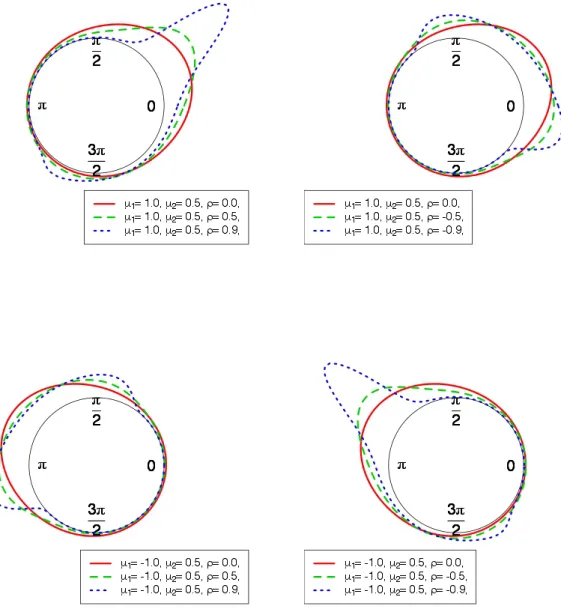
We provide some examples to illustrate the flexibility of the projected normal (PN) distribution. The PN density can be symmetric, asymmetric or possibly bimodal and apart form some special case, the interpretation of the parameters can be difficult. The number of modes and the shape depend on the value of the all parameters and different sets of parameters can give really similar shapes. As a general comment we highlight thatµ1 and µ2 are the means of the two Cartesian coordinatesz1 and z2 and are respectively connected to the cosine and sine of the circular variable. By fixing σ12 = 1
and ρ = 0, the resulting distribution is unimodal and symmetric and if µ1 =µ2 = 0 the distribution
becomes a circular uniform. Departure from zero for the two means, in the case of identity covariance matrix, creates one mode in the trigonometric quadrant with the same sign of the means, e.g. ifµ1>0
and µ2 <0 then the mode is in the quadrant with positive cosine and negative sine; higher values of
a mean attract the mode to its correspondent axis. By allowing the ρ parameter to vary, we obtain very flexible shapes. The resulting distribution shows asymmetry with more mass of probability near the axis with the highestµ. By increasing |ρ|, bimodality is detected, Figure 1. Moreover, for σ12<1 the modes are closer to the sine axis; while forσ21 >1 the modes are closer to the cosine axis.
3
THE CIRCULAR-LINEAR GENERAL PROJECTED NORMAL
HIDDEN MARKOV MODEL
3.1 The Model
Let T = {0,1, . . . , T −1, T}, in this paper we consider a bivariate time series [x,y] = {[xt, yt];t ∈
T \{0}}with circular,xt, and linear,yt, components. Our aim is to jointly classify [xt, yt] inK classes,
generally called regimes or states, with a HMM-based classifier.
Letπk,h indicates the probability to move from statek to stateh and letξtk be an indicator variable
such that if we are in state k on timet it is 1, otherwise is 0. Then f(ξth = 1|ξt−1k = 1) = πk,h and
we set f(ξ0k) =πk. We indicate with
π= π1,1 π1,2 · · · π1,K π2,1 π2,2 · · · π2,K · · · · πK,1 πK,2 · · · πK,K , K X h=1 πk,h= 1, k= 1,2, . . . , K,
the transition matrix that governs the evolution of the Markov chain, π0 = [π1, π2, . . . , πK]0 and ξ= [ξ0,ξ1, . . . ,ξT]0 whereξt= [ξt1, ξt2, . . . , ξtK]0.
Letnk,h=PTt=1ξt−1kξthbe the number of times we move from statekto stateh, the joint density of
the vector of states isf(ξ|π,π0) =QKk=1πkξ0kQKk=1QKh=1πnk,hk,h. In the literature on HMM for
circular-linear variables, see for example Bullaet al.(2012) and Holzmannet al.(2006), it is generally assumed that conditioning to the latent vectorξ, the pairs [xt, yt] and [xg, yg] are independent ifg6=tand at the
Figure 1: Shape of the projected normal distribution forσ2 = 1 and different values ofρ,µ1 and µ2
same time xt⊥yt. As a result, the conditional distribution of the observed process, given the latent
process, takes the form of a product density, sayf(x,y|ξ) =QK
k=1
QT
t=1[f(xt|ξtk = 1)f(yt|ξtk = 1)] ξtk.
We maintain the so-called conditional independence property: given the hidden state at time t, the distribution of the observation at this time is fully determined, but we relax the assumption on in-dependence between the circular and linear variables observed at the same time. Thus, we get a multivariate conditional distribution f(x,y|ξ) =QK
k=1 QT t=1f(xt, yt|ξtk = 1)ξtk. Let Zt|ξtk = 1 ∼ N(µk,Σk), with Zt = Zt1 Zt2 , µk = µk1 µk2 Σk = σ2k1 σk1ρk σk1ρk 1 and let Rt = ||Zt||. We define Xt as the radial projection of Zt: Xt = arctan∗ZZ12 and then Xt|ξtk =
1 ∼ P N2(µk,Σk). We can write easily the joint density of [Xt, Rt] that is the density that arises
by a variable transformation from the bivariate normal Zt to its polar system representation. Let φh(ζ|M,V) be the probability density function of a h-variate normal distribution with meanM and
covariance matrixV evaluated in ζ, then
We built the (conditional) joint density f(xt, yt|ξtk = 1) = f(yt|xt, ξtk = 1)f(xt|ξtk = 1) as a
marginalization over the latent variable Rt: f(xt, yt|ξtk = 1) =
R
rtf(yt|xt, rt, ξtk = 1)f(xt, rt|ξtk =
1)drt, where f(xt, rt|ξtk = 1) is specified in equation (1) and yt|xt, rt, ξtk = 1 is defined through
a circular-linear regression. However, there is not an obvious and standard way to formalize the relations between circular and linear variables. Jammalamadaka and SenGupta (2001) propose a flexible approach using trigonometric polynomials while Mardia (1976) and Johnson and Wehrly (1978) proposed a regression where the covariates are the sine and cosine components of the circular variable. Here, following Wanget al.(2014), we specify the relation asyt=γk0+γk1rtcosxt+γk2rtsinxt+tk,
with tk ∼ N(0, σky). Thus, yt|xt, rt, ξtk = 1 is distributed as a normal variable with mean γk0 + γk1rtcosxt+γk2rtsinxtand variance σky2 . Note that the regression can be seen as a linear regression
between yt and the inline variables rtcosxt and rtsinxt. This type of representation gives more
flexibility to the circular linear regression than the ones proposed by Mardia (1976) and Johnson and Wehrly (1978). Notice that with thert variable, for a given value of the circular variable at different
time point, say xt =xt0, t 6= t0, the relation between xt and yt and xt0 and yt0 can be different as it
depends on the realization of the non observed variable rt.
Then we have that
f(xt, yt|ξtk = 1) = φ1(yt|γk0, σ2ky)φ2(µk|02,Σk) h mtkΦ mtk √ vtk +φ1(mtk|0, vtk) i φ1(mtk|0, vtk) , (2)
where Φ is the cumulative density function of a standard normal distribution,w=
cosxt sinxt ,vtk = c2 tk σ2 ky +w0tΣ−1k wt −1 , mtk = vtk ctk(yt−γk0) σ2 ky +wt0Σ−1k µk and ctk =w0t γk1 γk2
. The Circular Linear General projected normal (CL-GPN) distribution with parameters [µk1, µk2, σk12 , ρk, γk0, γk1, γk2, σ2ky]0
is thus defined in (2). In this setting the parameter γk1 and γk2 govern the dependency between the
two variables (linear and circular),γk1 is connected to the correlation between the linear variable and
the cosine of the circular, γk1 is connected to the correlation between the linear variable and the sine
of the circular.
Wang et al. (2014) and Wang and Gelfand (2012) argue that working with the projected normal density is not easy and its form is practically intractable (to see the closed form of the PN density see Wang and Gelfand (2012)). Since the CL-GPN is based on the PN, is itself an intractable distribution and the implementation of the MCMC algorithm can be difficult. However the introduction of rt is
of practical use as it simplifies the implementation of the MCMC algorithm, see Section 3.3.
3.2 Posterior Inference
LetΨbe the vector of all the parameters of the CL-GPN in all theK regimes, we have the following posterior distribution f(π,ξ,π0,Ψ,r|x,y) = f(r,x,y|Ψ,ξ)f ξ−0|ξ0,π f(π)f(ξ0|π0)f(π0)f(Ψ) f(x,y) where r = [r1, . . . , rt]0 and f(x,y,r|ξ) = QKk=1 QT t=1f(xt, rt, yt|ξtk = 1)ξtk. As prior distribution we assume: µki ∼ N(·,·), σ2k1 ∼ IG(·,·), ρk ∼ N(·,·)I(−1,1), σky2 ∼ IG(·,·), γkj ∼ N(·,·) for k =
1, . . . , K, i= 1,2, j= 1,2,3, whereIG(·,·) indicates the Inverse Gamma distribution,π0 ∼Dir(·) and πk,.∼Dir(·) whereDir(·) indicates the Dirichlet distribution andπk,. is thekth row ofπ: we assume πk⊥πk0 ifk6=k0. The prior specification allows us to marginalized overπandπ0reducing ofK2the
number of parameters to simulate and leads to a more efficient and stable algorithm (see Banerjeeet al.
(2004) and Section 3.3). Note that we can always sample from f(πk,.|x,y) = Pξf(πk,.|ξ)f(ξ|x,y)
and f(π0|x,y) = Pξf(π0|ξ)f(ξ|x,y) given the set of B posterior samples {ξb}Bb=1 of ξ, with an
MCMC integration. For each sample ξb we draw a sample from πbk,.|ξb ∼ Dir(β+ PT
t=2 ξt−1kb ξbt1, . . . , β +PT
t=2ξt−1kb ξtKb ) and one from πb0|ξb ∼ Dir β+ξ01b , . . . , β+ξ0Kb
. The sets {πbk,.}B b=1 and
{πb0}B
b=1 are draw from their respectively marginal posterior distributions. The posterior distribution
we will work with is then
f(ξ,Ψ,r|x,y) = f(r,x,y|Ψ,ξ)f(Ψ)f(ξ−0|ξ0)f(ξ0) f(x,y) . wheref(ξ−0|ξ0) = R πf ξ−0|ξ0,π f(π)dπand f(ξ0) =R π0f(ξ0|π0)f(π0)dπ0 can be computed in closed form: f(ξ−0|ξ0) = Γ(Kβ)K Γ(β)K2 QK k=1 QK h=1Γ(nk,h+β) QK k=1Γ(nk−ξT ,k+Kβ) and f(ξ0) = 1 K 3.3 Computational Details
Model parameters are estimated with a MCMC algorithm. More precisely the µs, γs, σy2s and ξ
are simulated with a Gibbs sampler while the remaining parameters require the introduction of a Metropolis step. The full conditionals ofµs and γs are normal distributions, those ofσ2ys are inverse gamma. The full conditionals for the latent variables ξt, t ∈ T are multinomial and the vector of probabilities depends on the entire vector of ξ−t = ξ\{ξt}. More precisely, let s− and s+ be the
regimes on time t−1 and t+ 1, i.eξt−1s− = 1 andξt+1s+ = 1 respectively, let n−t
0 k = PT t=0 t6=t0 ξtk and n−tk,h0 =PT t=1 t6=t0,t6=t0+1 ξt−1kξt,h. If t∈ T \{0, T}. f(ξt|r,x,y,ξ−t,Ψ)∝ K Y k=1 n−ts−,k+β+as−,k,s+ n−t k,s++β n−tk −ξT,k+Kβ f(rt, xt, yt|ξt,Ψ)
whereas−,k,s+ assumes value 1 if s−=k=s+, 0 otherwise, while
f(ξT|r,x,y,ξ−T,Ψ)∝ K Y k=1 n−Ts−,k+β f(rT, xT, yT|ξT,Ψ). and f(ξ0|r,x,y,ξ−0,Ψ)∝ K Y k=1 n−0k,s+ +β n−0k −ξT,k+Kβ .
It is well known that the MCMC sampler for HMM tends to mix really slow (Andrieuet al., 2010). To speed up the convergence we try to find an optimal proposal distribution for the Metropolis step, that samplesK σ12variables,K ρvariables andT rvariables, using the algorithm described in Robert and Casella (2009), page 258. With the goal to speed up the MCMC convergence, as a general advice, is suggested to decrease the dimension of the parameters space, i.e. do as much marginalization as possible (Banerjee et al., 2004). In our model we found convenient to marginalize over the vectors
πk., k= 1, . . . , K and π0 but not overr. Marginalization overrdecreases significantly the number of
random variables to simulate but does not allow to have closed form for full conditional distributions of γk1,γk2 and µk. Without employing the Gibbs step, the MCMC algorithm becomes considerably
slower in moving toward its stationary distribution and then the computational burden increases as a larger number of iterations is required. On the other hand, marginalization over πk., k= 1, . . . , K
and π0 has impact only on the way we simulate ξt, t = 0,1, . . . , T, but their simulation is simple in
both cases, with or without πk., k= 1, . . . , K and π0, and can be carried out in a Gibbs step.
In the estimation step, we take into account the label-switching issue, common to all latent-class-based models. This problem occurs when exchangeable priors are used for the state specific parameters, which is common practice if there are not prior informations about the hidden states. In these cases, the posterior distribution is invariant to permutations of the state labels and, hence, the marginal posterior distributions of the state specific parameters are identical for all states. Therefore, direct inferences about the state specific parameters are not available from the MCMC output. Various approaches to deal with the label switching problem in finite mixture models have been proposed in the literature; see Jasra et al.(2005) for a recent review. To tackle the label switching we decide to use the post processing technique calledpivotal reordering, proposed in Spezia (2009) or in Marin and Robert (2013), Chapter 6.5.
3.4 Model Selection
To decide the number of regimes, we considered the idea of use the Reversible Jump (Green, 1995) or a non parametric approach, as the one proposed by Teh et al.(2004). However, our main goal is to demonstrate that the CL-GPN is suitable in a HMM Bayesian framework to model circular-linear variables. Thus, we do not want to further increase the complexity of an already highly complex model by introducingK as random variable.
Common model choice criteria are AIC, BIC, ICL and different classification-based information criteria which are minimized among a set of potential models. We evaluate these criteria using the set of parameters, among the MCMC draws, that maximize the posterior distribution (called maximum at posterior, MAP or MAP estimator) (Fr¨uhwirth Schnatter, 2006, Section 4.4.2, 7.1.4). Let ˜Ψbe the MAP estimator, we compute the BIC and AIC as BIC = −2 logfx,y|Ψ˜+ #parameters×
log(T) and AIC =−2 log
f x,y|Ψ˜ + 2×#parameters.
The BIC and AIC are generally criticized since they do not take into account the quality of classification of the variables in the K regimes. For classification purpose Biernacki et al. (2000) propose to use the ICL; an index based on the likelihood of observed variables and the vector of regimes indicator that is used by Celeux and Durand (2008) in a HMM context. We compute a BIC approximation of theICL=f(x,y|ξ˜,Ψ˜)−2 logf(˜ξ) + #parameters×log(T),(see for example Fr¨uhwirth Schnatter, 2006, pag. 214)
in the latter case, as suggested by McLachlan and Peel (2000), pag. 216, we first obtain an estimator of ξ, i.e. the MAP ˜ξ, and then, as for the BIC and AIC, we compute the ICL using the MAP estimator ofΨconditioning on the value ˜ξ.
4
SIMULATION STUDY
In this Section we carried out a simulation study to investigate the performance of the proposed approach in recovering model parameters and the hidden structure of the data. We empirically demonstrate that the CL-GPN can be used in presence of both unimodal or bimodal state-dependent circular distributions and that ignoring the dependencies between the circular and linear variable at a given time leads to a higher number of states.
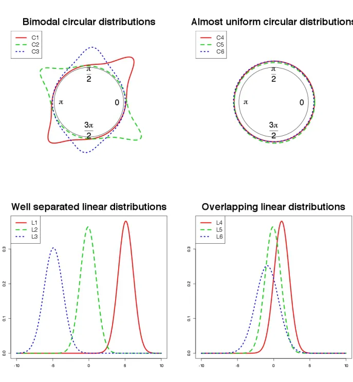
We plan the simulation study to cover schemes with different underlying null models assuming bimodal or almost uniform shapes for the circular variable, and overlapping or well-separated state-dependent distributions for the linear variable. On each simulated datasets, we estimate three models: 1) the CL-GPN model; 2) a constrained model, defined as diagonal CL-GPN (CL-DPN), withΣk=I2,
so that the state-dependent circular distribution is symmetric and unimodal; 3) a CL-GPN model with all theγk1 andγk2equal to zero, i.e. assuming independence between circular and linear variable given
the latent state (indicated as Ind-CL-GPN). 4.1 Designing the simulation study
For each null model, we simulated 200 datasets considering two time-series lengths, T = 500 and
T = 2000, with K = 3, ξ0 = 1 and transition matrix π with diagonal elements equal to 0.8 and extradiagonal elements equal to 0.1. The considered schemes are summarized in Figure 2, and are characterized by the following settings:
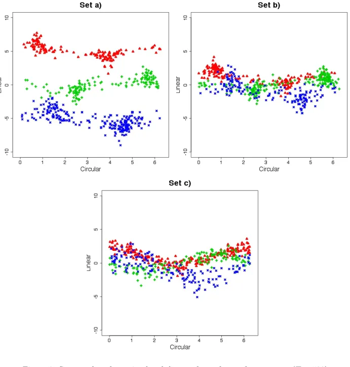
a) distributions C1 and L1, C2 and L2 and C3 and L3 are considered as state-dependent distribu-tions for the first, the second and the third regime, respectively. The joint representation through scatters is displayed in Figure 3. This scheme has bimodal state-dependent circular distributions and well separated linear ones. The following parameters are used to generate data:
µ= µ11 µ12 µ13 µ21 µ22 µ23 = 0.1 0.1 0.0 0.1 −1.0 −0.1
Figure 2: Marginal distributions used in the simulation examples. γ= γ01 γ02 γ03 γ11 γ12 γ13 γ21 γ22 γ23 = 5.0 0.0 −5.0 1.0 0.0 1.0 0.0 −1.0 1.0 σk12 = 1 k= 1 2 k= 2 0.1 k= 3 ; σ2ky = 0.1 k= 1 0.2 k= 2 0.5 k= 3 ; ρk= 0.9 k= 1 −0.9 k= 2 0.2 k= 3
b) this setting shares circular distributions with scheme a) while the state-dependent linear distri-butions are respectively the density L4, L5 and L6 of Figure 2. The joint representation through scatters is displayed in Figure 3. With respect to scheme a), we change the values ofγ:
γ= γ01 γ02 γ03 γ11 γ12 γ13 γ21 γ22 γ23 = 1.0 0.0 −1.0 1.0 0.0 1.0 0.0 −1.0 1.0
Figure 3: Scatter plot of one simulated dataset for each set of parameters (T = 500).
to have more overlapping state-dependent distributions for the linear variable.
c) the state-dependent distributions for the linear variable are the same as in scheme b), whilst the circular ones are respectively the density C4, C5 and C6 of Figure 2. The joint representation through scatters is displayed in Figure 3. In this case we simulate from a CL-DPN since we use σ112 =σ212 =σ132 = 1 and ρ1 = ρ2 =ρ3 = 0, i.e. the circular variable has state-dependent
unimodal (almost uniforms) distributions.
On each dataset we estimate models with K from 2 to 6 and assuming the following prior distri-butions: µki ∼ N(0,5), γkj ∼ N(0,5), ρk ∼N(0,5)I(−1,1), σ2k1 ∼IG(2,1)1,σ2ky ∼IG(2,1), β = 1
withi= 1,2 and j= 1,2,3; i.e. they do not depend on the regime. 1
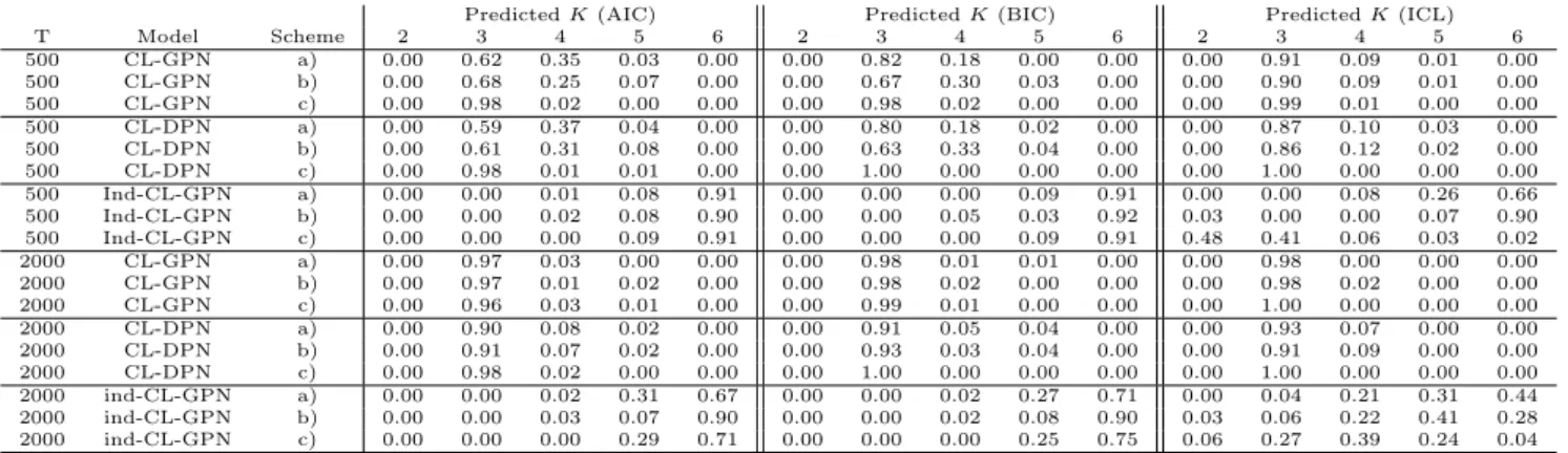
Table 1: Frequency distribution of predicted number of regimes
PredictedK(AIC) PredictedK(BIC) PredictedK(ICL)
T Model Scheme 2 3 4 5 6 2 3 4 5 6 2 3 4 5 6 500 CL-GPN a) 0.00 0.62 0.35 0.03 0.00 0.00 0.82 0.18 0.00 0.00 0.00 0.91 0.09 0.01 0.00 500 CL-GPN b) 0.00 0.68 0.25 0.07 0.00 0.00 0.67 0.30 0.03 0.00 0.00 0.90 0.09 0.01 0.00 500 CL-GPN c) 0.00 0.98 0.02 0.00 0.00 0.00 0.98 0.02 0.00 0.00 0.00 0.99 0.01 0.00 0.00 500 CL-DPN a) 0.00 0.59 0.37 0.04 0.00 0.00 0.80 0.18 0.02 0.00 0.00 0.87 0.10 0.03 0.00 500 CL-DPN b) 0.00 0.61 0.31 0.08 0.00 0.00 0.63 0.33 0.04 0.00 0.00 0.86 0.12 0.02 0.00 500 CL-DPN c) 0.00 0.98 0.01 0.01 0.00 0.00 1.00 0.00 0.00 0.00 0.00 1.00 0.00 0.00 0.00 500 Ind-CL-GPN a) 0.00 0.00 0.01 0.08 0.91 0.00 0.00 0.00 0.09 0.91 0.00 0.00 0.08 0.26 0.66 500 Ind-CL-GPN b) 0.00 0.00 0.02 0.08 0.90 0.00 0.00 0.05 0.03 0.92 0.03 0.00 0.00 0.07 0.90 500 Ind-CL-GPN c) 0.00 0.00 0.00 0.09 0.91 0.00 0.00 0.00 0.09 0.91 0.48 0.41 0.06 0.03 0.02 2000 CL-GPN a) 0.00 0.97 0.03 0.00 0.00 0.00 0.98 0.01 0.01 0.00 0.00 0.98 0.00 0.00 0.00 2000 CL-GPN b) 0.00 0.97 0.01 0.02 0.00 0.00 0.98 0.02 0.00 0.00 0.00 0.98 0.02 0.00 0.00 2000 CL-GPN c) 0.00 0.96 0.03 0.01 0.00 0.00 0.99 0.01 0.00 0.00 0.00 1.00 0.00 0.00 0.00 2000 CL-DPN a) 0.00 0.90 0.08 0.02 0.00 0.00 0.91 0.05 0.04 0.00 0.00 0.93 0.07 0.00 0.00 2000 CL-DPN b) 0.00 0.91 0.07 0.02 0.00 0.00 0.93 0.03 0.04 0.00 0.00 0.91 0.09 0.00 0.00 2000 CL-DPN c) 0.00 0.98 0.02 0.00 0.00 0.00 1.00 0.00 0.00 0.00 0.00 1.00 0.00 0.00 0.00 2000 ind-CL-GPN a) 0.00 0.00 0.02 0.31 0.67 0.00 0.00 0.02 0.27 0.71 0.00 0.04 0.21 0.31 0.44 2000 ind-CL-GPN b) 0.00 0.00 0.03 0.07 0.90 0.00 0.00 0.02 0.08 0.90 0.03 0.06 0.22 0.41 0.28 2000 ind-CL-GPN c) 0.00 0.00 0.00 0.29 0.71 0.00 0.00 0.00 0.25 0.75 0.06 0.27 0.39 0.24 0.04
4.2 Simulation Study Results
To evaluate the performance of AIC, BIC and ICL as selection criteria for the number of regimes, in Table 1 we report the frequency distribution of the predicted K under each simulation setting considered for the CL-GPN, CL-DPN and Ind-CL-GPN models. With respect to the CL-GPN model, we can observe that ICL performs considerably well in all cases. In fact, the predicted K is only occasionally different from the true one, and, when this happens, the former is always larger than the latter. On the other hand, AIC and BIC have an excellent behavior with the exception of the cases
T = 500, schemes a) and b). As may be expected, these criteria perform better as the amount of information in the data increases.
Ignoring the (state-dependent) correlation between circular and linear measurements may strongly affect the hidden structure. Indeed, by looking at information criteria for the Ind-CL-GPN model, we have that the latent structure is not well recovered and a higher number of regimes than expected is estimated. Of course, this affects parameter estimates and results interpretation, as a not needed number of (latent) regimes is identified in the data.
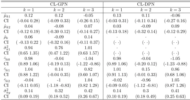
Here we briefly summarize the results of the simulation study for scheme c). By looking at parameters estimates (see Table 2), we have that the CL-GPN and the CL-DPN models lead essentially to the same results. Point estimates and credibility intervals are very close, suggesting that the CL-GPN distribution can be used whenever we cast doubts on the unimodality of circular distributions. Indeed, the CL-DPN distribution is a specific case of the CL-GPN one, in which conditional circular distribution are constrained to be unimodal.
To further resemble empirical situations, we randomly drop 10% observation of a randomly selected dataset simulated accordingly to the scheme c) with T = 500 and estimate the GPN and a CL-DPN models. Along with model parameters, we also simulate the missing observations. We compute the average continuous ranked probability score (CRPS) for both the circular (Grimitet al., 2006) and linear variable (Gneiting and Raftery, 2007) from the posterior samples of the missing observations, as well as the average prediction error (APE) for the circular variable (Jona Lasinioet al., 2012) and the mean squared error for the linear ones (MSE). With the CRPS we evaluate the model performance regarding the entire predictive distribution. APE and MSE allow us to measure the distance between the true values and the simulated ones. The CPRPs for the circular variable and the MSE are identical under the two models while the CRPS for the linear one is 0.66 under the CL-GPN and 0.67 under the CL-DPN and the APE is respectively 0.76 and 0.75 for the CL-GPN and the CL-DPN. Then the two models have the same performances in dealing with the missing values as well.
From the computational point of view, in the datasets with T = 2000 our C++ implementation of the model needs 1000000 iterations with a burnin of 700000 and a thin of 100 while with T = 500 the iterations needed are 800000, with a burnin of 400000 and again a thin of 100. The computational work for the simulation study and the real data application of Section 5, has been executed on the IT resources made available by ReCaS, a project financed by the MIUR (Italian Ministry for Education, University and Re-search) in the “PON Ricerca e Competitivit 2007-2013 - Azione I - Interventi di rafforzamento struttural” PONa3 00052, Avviso 254/Ric. The computational time are of the order
Table 2: posterior median estimates of the parameter (ˆ) and credibility intervals (CI) for scheme c) and T = 500 CL-GPN CL-DPN k= 1 k= 2 k= 3 k= 1 k= 2 k= 3 ˆ µk1 0.12 0.12 -0.05 0.13 0.11 -0.06 CI (-0.04 0.28) (-0.09 0.33) (-0.26 0.15) (-0.03 0.31) (-0.11 0.34) (-0.27 0.16) ˆ µk2 0.04 -0.08 0.07 0.03 -0.09 0.09 CI (-0.12 0.19) (-0.30 0.12) (-0.14 0.27) (-0.13 0.18) (-0.32 0.14) (-0.12 0.29) ˆ ρk 0.06 -0.09 0.14 · · · CI ( -0.13 0.22 ) (-0.32 0.16) (-0.11 0.37) (· ·) (· ·) (· ·) ˆ σ2 k1 0.94 0.76 1.01 · · · CI (0.65 1.35) (0.47 1.22) (0.63 1.57) (· ·) (· ·) (· ·) ˆ γk0 0.98 -0.04 -1.04 0.98 -0.04 -1.05 CI (0.89 1.06) (-0.19 0.13) (-1.22 -0.86) (0.89 1.06) (-0.20 0.12) (-1.23 -0.88) ˆ γk1 1.04 0.14 0.82 1.01 0.15 0.86 CI (0.88 1.22) (-0.04 0.35) (0.60 1.07) (0.91 1.13) (-0.01 0.33) (0.68 1.06) ˆ γk2 -0.04 -1 1.04 -0.02 -0.96 1.05 CI (-0.11 0.05) (-1.18 -0.83) (0.82 1.28) (-0.09 0.05) (-1.12 -0.81) (0.87 1.26) ˆ σky2 0.14 0.32 0.42 0.14 0.3 0.41 CI (0.09 0.19) (0.18 0.52) (0.26 0.67) (0.10 0.19) (0.18 0.49) (0.25 0.63)
of 1 hour for T = 500 and 5 hours for T = 2000. All the results shown are from MCMC chains that reach the convergence, checked using the standard tool on the R package coda.
5
REAL DATA EXAMPLE
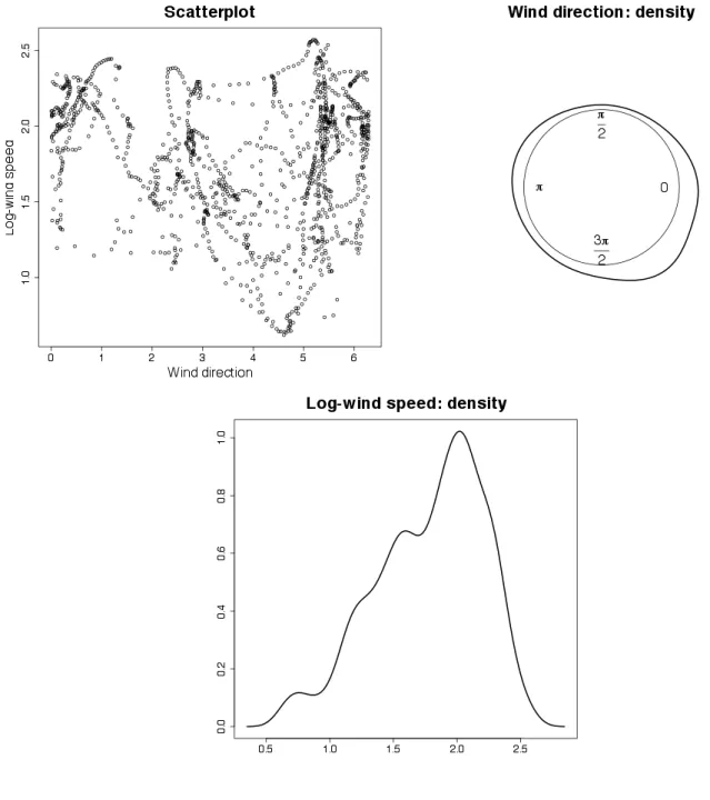
Finally, we apply the CL-GPN hidden Markov model to a bivariate time series of wind directions and (log-transformed) speeds. Data are recorded on a semi-hourly base from 12/12/2009 to 12/1/2010 in Ancona (Italy) at a bouy located in the Adriatic Sea 30km from the coast (see Figure 4). Data are recorded onT = 1500 times and have been previously analysed by Bullaet al. (2012).
As often arise in environmental studies, data are not complete. 213 and 210 missing values are recorded for directions and speeds, respectively; 125 profiles are completely missing.
During wintertime, relevant wind events in the Adriatic Sea are typically generated by the south-eastern Sirocco, the north-south-eastern Bora and the north-western Maestral. Sirocco arises from a warm, dry, tropical air mass that is pulled northwards by low-pressure cells moving eastwards across the Mediterranean Sea. By contrast, Bora episodes occur when a polar high-pressure area sits over the snow-covered mountains of the interior plateau behind the coastal mountain range and a calm low-pressure area lies further south over the warmer Adriatic. Finally, the Maestral is a sea-breeze wind blowing northwesterly when the east Adriatic coast gets warmer than the sea. While Bora and Sirocco episodes are usually associated with high-speed flows, Maestral is in general linked with good meteorological conditions. Hence, the marginal distribution of (log-transformed) wind speed may be interpreted as the result of mixing different wind-speed regimes.
As for the simulation examples, we look at the AIC, BIC and ICL to select the appropriated number of components. The ICL suggest to useK = 3 while the AIC and BICK = 4. To help decide between the two number of regimes, we look ar their predictive ability, the CRPScand APE highlight
loss of predictive ability on the circular variable if we choose K = 4 (CRPSc=0.59 and APE=0.75
with K = 4 while CRPSc=0.34 and APE= 0.35 with K = 3). For the linear variable, looking at
the values of CRPSl and MSE, there is a small difference between K = 3 and K = 4 however both
CRPSl and MSE favour K = 3 (CRPSl=0.17 and APE=0.39 with K = 4 while CRPSl=0.16 and
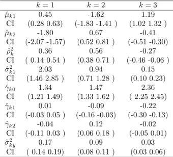
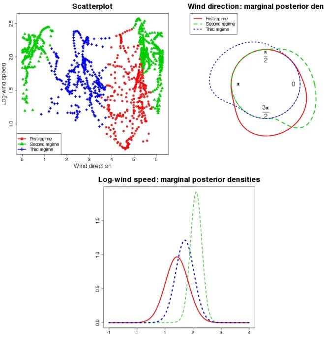
APE= 0.34 with K = 3). We decide to adopt K = 3, that is also the choice of Bulla et al. (2012) following their suggestion that three regimes provide well-separated and more interpretable states. The resulting classification is displayed in Figure 5 and all the credibility intervals and point estimates of the parameters are in Table 3. The estimated transition probabilities are displayed in Table 4. As
Figure 4: Real data.
expected, the transition probability matrix is essentially diagonal, reflecting the temporal persistence of the regimes, i.e. of wind conditions . Furthermore, the small off-diagonal transition probabilities between states indicate that direct transitions between Sirocco and Bora episodes are very unlikely. The model hence confirms that the Adriatic Sea typically alternates relevant wind events with periods of good conditions.
For a more clear interpretation of the state dependent distributions, we compute some feature of the CL-GPN distribution. In detail, we look at the posterior marginal mean and variance of the linear distribution for each regime (¯µky and ¯σky2 ), the circular mean (¯µkx) and concentration(¯gkx) of
the circular variable and a measure of correlation between the circular and linear variables ( ¯ρ2kxy) as in Mardia and Jupp (1999), pag. 245. Point estimates and credibility intervals are provided in Table 5).
The regimes are ordered accoridng to the marginal log-wind speed. In the three regimes the point estimates are respectively ˆµky = 1.42,1.70,2.11 (which correspond to 4.14m/s, 5.47m/s,8.25m/s in
the natural scale). With the increases of the velocity, the distribution becomes more concentrated: the marginal linear variance, ˆσ¯ky2 , is respectively 0.17,0.11,0.04, for a plot of the distributions see
Table 3: Real data: posterior median estimates of the parameter (ˆ) and credibility intervals (CI) k= 1 k= 2 k= 3 ˆ µk1 0.45 -1.62 1.19 CI (0.28 0.63) (-1.83 -1.41 ) (1.02 1.32 ) ˆ µk2 -1.80 0.67 -0.41 CI (-2.07 -1.57) (0.52 0.81 ) (-0.51 -0.30) ˆ ρ2 k 0.36 0.56 -0.27 CI ( 0.14 0.54 ) (0.38 0.71 ) (-0.46 -0.06 ) ˆ σ2 k1 2.03 0.94 0.15 CI (1.46 2.85 ) (0.71 1.28 ) (0.10 0.23) ˆ γk0 1.34 1.47 2.36 CI (1.21 1.49) (1.33 1.62 ) ( 2.25 2.45) ˆ γk1 0.01 -0.09 -0.22 CI (-0.03 0.05 ) (-0.16 -0.03) (-0.30 -0.13) ˆ γk2 -0.04 0.12 -0.02 CI (-0.11 0.03 ) (0.06 0.18 ) (-0.05 0.01) ˆ σ2 ky 0.17 0.09 0.03 CI ( 0.14 0.19) (0.08 0.11 ) (0.03 0.06)
Table 4: Real data: Transition matrix
Destination state 1 2 3 1 0.96 0.02 0.02 (0.94, 0.97) (0.01, 0.04) ( 0.01, 0.04) Origin state 2 0.02 0.97 0.00 (0.01 0.04) ( 0.95, 0.98) (0.00, 0.01) 3 0.02 0.00 0.98 (0.01, 0.03) (0.00, 0.01) (0.97, 0.99)
Table 5: Real data: posterior median estimates (ˆ) and credibility intervals (CI) of the features of the distribution CL-GPN k= 1 k= 2 k= 3 ˆ ¯ µkx 4.98 2.7 6.04 CI (4.81 5.16) (2.55 2.83) (5.90 6.19) ˆ ¯ gkx 0.78 0.83 0.82 CI (0.71 0.84) (0.77 0.87) (0.76 0.86) ˆ ¯ µky 1.42 1.70 2.11 CI (1.34 1.50) (1.63 1.78) (2.02 2.20) ˆ ¯ σ2 ky 0.17 0.11 0.04 CI (0.15 0.20) (0.09 0.12) (0.03 0.07) ˆ ¯ ρ2 kxy 0.02 0.05 0.05 CI (0.00 0.10) (0.00 0.18) (0.00 0.17)
Figure 5: Real data classification.
Figure 5. The circular mean is 4.98 in the first regime, north-westerly Maestral episodes, 2.70 in the second, south-eastern Sirocco, and 6.04 in the third, northern Bora jets, on the first regime the circular marginal distribution is less concentrated than in the others (0.78 for k= 1, 0.83 for k= 2 and 0.82 fork= 3).
The correlations between the circular and linear variables are weak in all the regimes: ˆρ¯2kxy is 0.02 in the first and 0.05 in the others. Under the hypothesis of no correlation, i.e. ¯ρ2kxy = 0, the statistic ˜F = ρ¯
2
kxy(n−1) 1−¯ρ2
kxy
is distributed as a F2,T−3 where in our case T = 1500. The lower limits of
the 95% credibility intervals of the posterior distributions of ˜F are 1.24, 4.80 and 4.95 in the calm, transition and storm conditions respectively, and the 95% percentile of F2,T−3 is 3.00. Accordingly,
circular-linear correlations are significant in the transition and storm conditions only. This result is not present at all in previous analyses. This can be seen also with the value ofγk1 and γk2 in Table 3.
In the first regime ˆγ11= 0.01 and ˆγ12=−0.04, both credibility intervals contain the 0. In the second
there is a negative relation between the linear variable and the cosine of the circular one (γ1=−0.09)
linear and circular variable is on the cosine direction (γ1=−0.22).
We estimate the model using 1000000 iterations, a burnin of 700000 and a thin of 100. Here again we checked the convergence of the MCMC chain using the standard tool on the R package coda.
6
Discussion
In this work we introduce, for the first time, the CL-GPN distribution in a Bayesian HMM framework and we present the explicit expression of the CL-GPN likelihood. This approach allows to easily model multivariate processes with mixed support (circular-linear), by combining the bivariate representation of the circular component (i.e. the projected normal distribution) and a Gaussian distribution for the linear part. Here we considered one circular and one linear variable although it is fairly easy to extend the proposed model to more than one linear component.
The Bayesian framework allows us to overcome identifiability issues and computational problems that may arise in the classical setting. Several implementation novelties are introduced to speed up al-gorithms convergence. We use an adaptive Metropolis whenever a Gibbs sampler is not implementable (section 3.3). Furthermore we marginalize the transition matrix so to avoid its estimation to reduce the problem size obtaining it as an a posteriori byproduct (Section 3.2) and we provide evidence that the marginalization does not affect parameters estimation. We also demonstrate that assuming con-ditional independence between the circular and linear variable can make difficult to correctly estimate the number of regimes.
We applied this methodology to wind data confirming previously obtained results and highlighting new data features. Circular parameters interpretation is not straightforward, however this does not limit the inferential richness of the model. Using MCMC simulations posterior circular mean and concentration can be derived, as well as the circular-linear correlation. Of course, different areas of application can be considered for the proposed approach, e.g. animal movement modelling (Langrock
et al., 2014) and driving behaviour (Jackson et al., 2014).
Further developments will include the extension to more than one circular variable. This extension requires a careful definition of correlation between circular variables that is not straightforward under the projected normal distribution. Another interesting extension of the proposed approach is to allow the estimation of the number of states along with the model parameters. The latter can be obtained using a hierarchical Dirichlet process on the states or a reversible jump.
A crucial assumption of our model is that the temporal dependence is well described by a first order Markov chain, i.e. the sojourn time is geometrical. If we want to allow for different sojourn time distributions with finite support the HMM formulation is exact. Similarly by allowing the number of hidden states to grow with the sample size, we can allow for continuos time, i.e. the hidden distribution can be approximated with arbitrary accuracy using the proposed model. This can be seen as a possible solution to computational issues arising with continuous-valued latent models (Langrocket al., 2012b).
References
Alf`o M, Maruotti A, 2010. A hierarchical model for time dependent multivariate longitudinal data. In Palumbo F, Lauro CN, Greenacre MJ (eds.), Data Analysis and Classification, Studies in Classifi-cation, Data Analysis, and Knowledge Organization, Springer Berlin Heidelberg, 271–279.
Andrieu C, Doucet A, Holenstein R, 2010. Particle Markov chain Monte Carlo methods. Journal of the Royal Statistical Society: Series B (Statistical Methodology) 72(3): 269–342.
Banerjee S, Gelfand AE, Carlin BP, 2004.Hierarchical Modeling and Analysis for Spatial Data. Chap-man and Hall/CRC.
Bartolucci F, Farcomeni A, 2009. A multivariate extension of the dynamic logit model for longitu-dinal data based on a latent Markov heterogeneity structure. Journal of the American Statistical Association 104(486): 816–831.
Bartolucci F, Farcomeni A, 2010. A note on the mixture transition distribution and hidden Markov models. Journal of Time Series Analysis 31(2): 132–138.
Bartolucci F, Farcomeni A, Pennoni F, 2012.Latent Markov Models for Longitudinal Data. Chapman and Hall.
Bartolucci F, Farcomeni A, Pennoni F, 2014. Latent Markov models: a review of a general framework for the analysis of longitudinal data with covariates.TEST to appear.
Bartolucci F, Pennoni F, Vittadini G, 2011. Assessment of school performance through a multilevel latent Markov Rasch model. Journal of educational and behaviour statistics 36(4): 491–522.
Baudry JP, Raftery AE, Celeux G, Lo K, Gottardo R, 2010. Combining mixture components for clustering. Journal of Computational and Graphical Statistics 19(2): 332–353.
Biernacki C, Celeux G, Govaert G, 2000. Assessing a mixture model for clustering with the integrated completed likelihood. IEEE Trans. Pattern Anal. Mach. Intell.22(7): 719–725.
Bulla J, Lagona F, Maruotti A, Picone M, 2012. A multivariate hidden Markov model for the iden-tification of sea regimes from Incomplete skewed and circular time series. Journal of Agricultural, Biological, and Environmental Statistics 17(4): 544–567.
Capp´e O, Moulines E, Ryden T, 2005.Inference in Hidden Markov Models. Springer Series in Statistics, Springer.
Celeux G, Durand JB, 2008. Selecting hidden Markov model state number with cross-validated like-lihood. Comput. Stat. 23(4): 541–564.
Dannemann J, 2012. Semiparametric hidden Markov models.Journal of Computational and Graphical Statistics 21(3): 677–692.
Fr¨uhwirth Schnatter S, 2006.Finite Mixture and Markov Switching Models. Springer Verlag.
Geweke J, Amisano G, 2011. Hierarchical Markov normal mixture models with applications to financial asset returns. Journal of Applied Econometrics 26(1): 1–29.
Gneiting T, Raftery AE, 2007. Strictly proper scoring rules, prediction, and estimation. Journal of the American Statistical Association 102(477): 359–378.
Green PJ, 1995. Reversible jump Markov chain monte carlo computation and Bayesian model deter-mination. Biometrika 82(4): 711–732.
Grimit EP, Gneiting T, Berrocal VJ, Johnson NA, 2006. The continuous ranked probability score for circular variables and its application to mesoscale forecast ensemble verification.Quarterly Journal of the Royal Meteorological Society 132: 2925–2942.
Holzmann H, Munk A, Suster M, Zucchini W, 2006. Hidden Markov models for circular and linear-circular time series. Environmental and Ecological Statistics 13(3): 325–347.
Jackson J, Albert P, Zhiwei Z, 2014. A two-state mixed hidden Markov model for risky teenage driving behavior. The Annals of Applied Statistics To appear.
Jammalamadaka SR, SenGupta A, 2001. Topics in Circular Statistics. World Scientific.
Jasra A, Holmes CC, Stephens DA, 2005. Markov chain Monte Carlo methods and the label switching problem in Bayesian mixture modeling. Statistical Science 20(1): 50–67.
Johnson RA, Wehrly TE, 1978. Some Angular-Linear Distributions and Related Regression Models.
Jona Lasinio G, Gelfand A, Jona Lasinio M, 2012. Spatial analysis of wave direction data using wrapped Gaussian processes. Annals of Applied Statistics 6(4): 1478–1498.
Kato S, Shimizu K, Shieh GS, 2008. A circular-circular regression model.Statistica Sinica18: 633–645.
Lagona F, Maruotti A, Picone M, 2011.A Non-homogeneous Hidden Markov Model For The Analysis Of Multi-pollutant Exceedances Data — InTechOpen, chapter 10. INTECH, University Campus STeP Ri Slavka Krautzeka 83/A 51000 Rijeka Croatia, 207–222.
Lagona F, Picone M, 2011. A latent-class model for clustering incomplete linear and circular data in marine studies. Journal of Data Science 9(4).
Lagona F, Picone M, 2012. Model-based clustering of multivariate skew data with circular components and missing values. Journal of Applied Statistics 39(5): 927–945.
Lagona F, Picone M, Maruotti A, Cosoli S, 2014. A hidden Markov approach to the analysis of space-time environmental data with linear and circular components. Stochastic Environmental Research and Risk Assessment to appear.
Langrock R, King R, Matthiopoulos J, Thomas L, Fortin D, Morales JM, 2012a. Flexible and practical modeling of animal telemetry data: hidden Markov models and extensions. Ecology 93(11): 2336– 2342.
Langrock R, Kneib T, Michelot T, 2014. Markov-switching generalized additive models.ArXiv e-prints
.
Langrock R, MacDonald IL, Zucchini W, 2012b. Some nonstandard stochastic volatility models and their estimation using structured hidden Markov models. Journal of Empirical Finance 19(1): 147 – 161.
Langrock R, Swihart BJ, Caffo BS, Punjabi NM, Crainiceanu CM, 2013. Combining hidden Markov models for comparing the dynamics of multiple sleep electroencephalograms. Statistics in Medicine
32(19): 3342–3356.
Mardia KV, 1976. Linear-Circular Correlation Coefficients and Rhythmometry.Biometrika 63(2).
Mardia KV, Jupp PE, 1999.Directional Statistics. John Wiley and Sons.
Marin J, Robert C, 2013.Bayesian Essentials with R. Springer Texts in Statistics, Springer New York. Martinez-Zarzoso I, Maruotti A, 2013. The environmental kuznets curve: functional form, time-varying
heterogeneity and outliers in a panel setting. Environmetrics 24(7): 461–475.
Maruotti A, 2011. Mixed hidden Markov models for longitudinal data: An overview. International Statistical Review 79(3): 427–454.
McLachlan C, Peel D, 2000.Finite Mixture Models. John Wiley and Sons, New York.
Robert CP, Casella G, 2009. Introducing Monte Carlo Methods with R. Springer, Berlin, Heidelberg. Ryd`en T, 2008. Em versus Markov chain Monte Carlo for estimation of hidden Markov models: a
computational perspective. Bayesian Analysis 3(4): 659–688.
Ryd`en T, Titterington DM, 1998. Computational Bayesian analysis of hidden Markov models.Journal of Computational and Graphical Statistics 7(2): 194–211.
Spezia L, 2009. Reversible jump and the label switching problem in hidden Markov models.Journal of Statistical Planning and Inference 139(7): 2305 – 2315.
Spezia L, 2010. Bayesian analysis of multivariate Gaussian hidden Markov models with an unknown number of regimes.Journal of Time Series Analysis 31(1): 1–11.
Teh YW, Jordan MI, Beal MJ, Blei DM, 2004. Hierarchical Dirichlet processes. Journal of the Amer-ican Statistical Association 101: 1566–1581.
Wang F, Gelfand A, 2012. Directional data analysis under the general projected normal distribution.
Statistical Methodology 10(1): 113 – 127.
Wang F, Gelfand A, 2014. Modeling space and space-time directional data using projected Gaussian processes. Journal of the American Statistical Association to appear.
Wang F, Gelfand A, Jona Lasinio G, 2014. Joint spatio-temporal analysis of a linear and a directional variable: Space-time modeling of wave heights and wave directions in the adriatic sea. Statistica Sinica to appear.
Yildirim S, Singh SS, Dean T, Jasra A, 2014. Parameter estimation in hidden Markov models with intractable likelihoods using sequential monte carlo.Journal of Computational and Graphical Statis-tics to appear.
Zhang Q, Snow Jones A, Rijmen F, Ip EH, 2010. Multivariate discrete hidden Markov models for domain-based measurements and assessment of risk factors in child development. Journal of Com-putational and Graphical Statistics 19(3): 746–765.
Zucchini W, MacDonald I, 2009. Hidden Markov Models for Time Series: An Introduction Using R. Chapman & Hall/CRC Monographs on Statistics & Applied Probability, Taylor & Francis.